Global-scale wreath-building dynamos in stellar convection zones

Abstract

When stars like our Sun are young they rotate rapidly and are very magnetically active. We explore dynamo action in rapidly rotating suns with the 3-D MHD anelastic spherical harmonic (ASH) code. The magnetic fields built in these dynamos are organized on global-scales into wreath-like structures that span the convection zone. Wreath-building dynamos can undergo quasi-cyclic reversals of polarity and such behavior is common in the parameter space we have been able to explore. These dynamos do not appear to require tachoclines to achieve their spatial or temporal organization. Wreath-building dynamos are present to some degree at all rotation rates, but are most evident in the more rapidly rotating simulations.

1 Introduction

When stars like the Sun are young, they rotate quite rapidly. Observations of these young Suns indicate that they have strong surface magnetic activity and can undergo global-scale polarity reversals similar to the 22-year solar cycle. The magnetic fields observed at the surface of these stars are thought to originate in stellar dynamos driven in their convective envelopes. There, plasma motions couple with rotation to generate global-scale magnetic fields. Though correlations between the rotation rate of stars and their magnetic activity are observed (e.g., Pizzolato et al., 2003) it is at present unclear how the stellar dynamo process depends in detail on rotation.

Motivated by this rich observational landscape, we have explored the effects of more rapid rotation on 3-D convection and dynamo action in simulations of stellar convection zones. These simulations have been conducted using the anelastic spherical harmonic (ASH) code, a tool developed by a team of postdocs and graduate students working with Juri Toomre to study global-scale magnetohydrodynamic convection and dynamo action in stellar convection zones (e.g., Clune et al., 1999; Miesch et al., 2000; Brun et al., 2004, and contribution by Miesch in these proceedings).

We began our explorations of convection in rapidly rotating suns by exploring hydrodynamic simulations at a variety of rotation rates (Brown et al., 2008). These simulations capture the convection zone only, spanning from $0.72\>R_{\odot}$ to $0.97\>R_{\odot}$, and take solar values for luminosity and stratification but the rotation rate is more rapid. The total density contrast across such shells is about 25. In those simulations we found that the differential rotation generally becomes stronger as the rotation rate increases, while the meridional circulations appear to become weaker and multi-celled in both radius and latitude.

In this paper we review the dynamos we have found in our simulations of more rapidly rotating solar-type stars. These wreath-building dynamos form surprisingly organized structures in their convection zones (§2) and some even undergo quasi-cyclic magnetic reversals (§3). Wreath-building dynamos appear throughout the parameter space we have surveyed to date (§4). We close by reflecting on the challenges that lie ahead (§5).

2 A Dynamo with Magnetic Wreaths

Our first simulation discussed here, case D3, is of a star rotating three times faster than the Sun (Brown et al., 2010a). Vigorous convection in this simulation drives a strong differential rotation and achieves sustained dynamo action at relatively low magnetic Prandtl number; here Pm=$\nu/\eta$ is 0.5, where $\nu$ is the viscosity and $\eta$ is the magnetic diffusivity.

The magnetic fields created in this dynamo are organized on global-scales into banded wreath-like structures. These are shown for case D3 in Figure 1$a$. Two such wreaths are visible in the equatorial region, spanning the depth of the convection zone and latitudes from roughly $\pm 30^{\circ}$. The dominant component of the magnetism is the longitudinal field $B_{\phi}$, and the two wreaths have opposite polarities. Here the wreath in the northern hemisphere has negative polarity $B_{\phi}$ while the wreath in the southern hemisphere is positive in sense. The wreaths are not isolated flux structures; instead, magnetic fields meander in and out of each wreath, connecting them across the equator and to higher latitudes (Fig. 1$b$). The lack of visible magnetism in the polar regions reflects the relatively low magnetic Reynolds number associated with the convection (average fluctuating Rm’ is roughly 50 at mid-convection zone).

It has been a great surprise that such structures can exist in the convection zone of this simulation. Generally, it has been expected that convection should shred such structures or pump them downwards into a stable tachocline at the base of the convection zone. Here the entire domain is convectively unstable, and no such tachocline is present. The wreaths persist for long intervals in time, with the mean (longitudinally averaged) magnetic fields showing relatively little variation in time. The convection leaves its imprint on the wreaths, with the strongest downflows dragging the field towards the bottom of the convection zone. This is visible in the distinct waviness apparent in Figure 1. On the poleward edges the wreaths are wound up into the vortical convection there, and this appears to play an important role in regenerating the poloidal field.

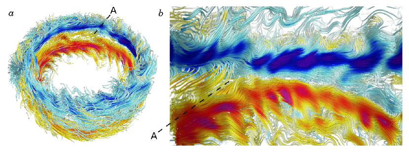
Figure 1: Magnetic wreaths in case D3. $(a)$ Full volume rendering of magnetic wreaths, showing entire simulation. Lines trace the vector magnetic field with color denoting amplitude and polarity of the longitudinal magnetic field $B_{\phi}$ (red or light tones, positive; blue or darker tones, negative). Rather than being simple flux surfaces, magnetic fields thread in and out of each wreath, connecting the wreaths across the equator and linking them to the polar regions. $(b)$ Zoom in view of region A showing cross-equatorial connectivity.

The magnetic wreaths are built by both the global-scale differential rotation and by the emf arising from correlations in the turbulent convection. Generally, the mean longitudinal magnetic field $\langle B_{\phi}\rangle$ in the wreaths is generated by the $\Omega$-effect: the stretching of mean poloidal field by the shear of differential rotation into mean toroidal field. Production of $\langle B_{\phi}\rangle$ by the differential rotation is balanced by turbulent shear and advection, and by ohmic diffusion on the largest scales.

The mean poloidal field is generated by the turbulent emf $E_{\mathrm{FI}}=\langle\boldsymbol{u^{\prime}}\times\boldsymbol{B^{\prime}}\rangle$, where the fluctuating velocity is $\boldsymbol{u^{\prime}}=\boldsymbol{u}-\langle\boldsymbol{u}\rangle$ and the fluctuating magnetic fields are $\boldsymbol{B^{\prime}}=\boldsymbol{B}-\langle\boldsymbol{B}\rangle$. In these simulations, $E_{\mathrm{FI}}$ is generally strongest at the poleward edge of the wreaths, centered at approximately $\pm 20^{\circ}$ latitude, whereas the $\Omega$-effect and $\langle B_{\phi}\rangle$ peak at roughly $\pm 15^{\circ}$ latitude. This spatial offset between $E_{\mathrm{FI}}$ and $\langle B_{\phi}\rangle$ means that the turbulent emf is not generally well represented by a simple $\alpha$-effect description, e.g.,

$$E_{\mathrm{FI}}=\langle\boldsymbol{u^{\prime}}\times\boldsymbol{B^{\prime}}\rangle|_{\phi}\neq\alpha\langle B_{\phi}\rangle$$ (1)

when $\alpha$ is a scalar quantity. This is true even when $\alpha$ is estimated from the kinetic and magnetic helicities present in the simulation. More sophisticated mean-field models may do much better at matching the observed emf $E_{\mathrm{FI}}$, and other terms in the mean-field expansion may play a significant role; in particular, the gradient of $\langle B_{\phi}\rangle$ is large on the poleward edges of the wreaths where $E_{\mathrm{FI}}$ is significant.

3 A Cyclic Dynamo in a Stellar Convection Zone

We turn now to a more rapidly rotating dynamo simulation, case D5, rotating five times faster than the Sun (Brown et al., 2010b). As in case D3, strong global-scale magnetic wreaths are built in the convection zone. Now however, the wreaths begin to show significant time-variation and undergo quasi-regular polarity reversals.

One such reversal is illustrated in Figure 2. Before the reversal (Fig. 2$a$), the wreaths look similar to those found in case D3, though here magnetism permeates the entire convection zone, including the polar regions where relic wreaths from the previous reversal are visible. The equatorial region shows significantly more connectivity and large fluctuations of $B_{\phi}$, with small knots of alternating polarity visible throughout. This cross-equatorial connectivity appears to play an important role in the reversal process. The magnetic fields built in case D5 attain somewhat larger amplitudes than those realized in case D3: here at mid-convection zone $B_{\phi}$ can reach $\pm 40\>$kG, while in case D3 the peak amplitudes were closer to $\pm 26\>$kG.

During the reversal (Fig. 2$b$), new wreaths of opposite polarity form near the equator while the old wreaths propagate towards the poles. This poleward propagation appears to be a combination of a nonlinear dynamo wave, arising from systematic spatial offsets between the generation terms for mean poloidal and toroidal magnetic field, and possibly a poleward-slip instability arising from magnetic stresses within the wreaths. After a reversal (Fig. 2$c$) the new magnetic wreaths grow in strength and dominate the equatorial region. In the polar regions the wreaths from the previous cycle begin to dissipate, reconnecting with the pre-existing flux there and being shredded by the turbulent convection there.

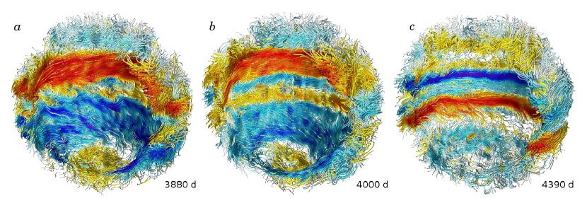
Figure 2: Global-scale magnetic reversal in case D5. $(a)$ Magnetic wreaths shown in field line tracing shortly before a polarity reversal, with positive polarity wreath above equator and negative polarity below. Volume shown spans slightly more than a full hemisphere with both polar caps visible where relic wreaths from the previous cycle remain visible. $(b)$ During a reversal, new wreaths with opposite polarity form at the equator while old wreaths migrate toward the poles. $(c)$ When the reversal completes, the polarity of the wreaths have flipped, with negative polarity wreath above the equator and positive below. Cancellation occurs in the polar regions and the old wreaths slowly dissipate. Times of snapshots are labeled.

Generally, the dynamo processes identified in case D3 serve to build the wreaths of case D5. As in case D3, before a reversal the turbulent emf $E_{\mathrm{FI}}$ that contributes to the mean poloidal field is generally largest on the poleward edge of the wreaths at latitudes above $\pm 20^{\circ}$, while the $\Omega$-effect and $\langle B_{\phi}\rangle$ peak at roughly latitude $\pm 15^{\circ}$. During a reversal both $E_{\mathrm{FI}}$ and the production of $\langle B_{\phi}\rangle$ associated with the $\Omega$-effect surf on the poleward edge of the wreaths as those structures move poleward. This systematic phase shift appears to contribute to that propagation.

4 Wreath-building Dynamos

The two simulations we have explored here, cases D3 and D5, are part of a much larger family of simulations that we have conducted exploring convection and dynamo action in younger suns. The properties of this broad family are summarized in Figure 3$a$. Indicated here are 26 simulations at rotation rates ranging from $0.5\>\Omega_{\odot}$ to $15\>\Omega_{\odot}$. At individual rotation rates (e.g., $3\>\Omega_{\odot}$), further simulations explore the effects of lower magnetic diffusivity $\eta$ and hence higher magnetic Reynolds numbers. Some of these follow a path where the magnetic Prandtl number Pm is fixed at 0.5 (triangles) while others sample up to Pm=4 (diamonds). The most turbulent simulations have fluctuating magnetic Reynolds numbers of about 500 at mid-convection zone. Wreath-building dynamos are achieved in most simulations (17), though a smaller number do not successfully regenerate their mean poloidal fields (9, indicated with crosses). Very approximate regimes of dynamo behavior are indicated, based on the time variations shown by the different classes of dynamos.

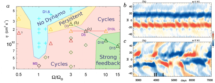
Figure 3: Wreath-building dynamos. $(a)$ Parameter space showing variety of wreath-building dynamos currently explored. Magnetic diffusivity $\eta$ and rotation rate $\Omega$ are shown for dynamo simulations at rotation rates ranging sampling $0.5$–$15\Omega_{\odot}$, with very approximate dynamo regimes shown. In some regions, magnetic Reynolds numbers are too low to sustain dynamo action, while in other regions persistent magnetic wreaths form which do not show evidence for cycles. At higher magnetic Reynolds numbers (occurring here at low $\eta$ or high $\Omega$), wreaths typically undergo quasi-cyclic reversals. At the highest rotation rates the Lorentz force can substantially modify the differential rotation, but dynamo action is still achieved. Cases with question marks show significant time-variation but have not been computed for long enough to definitively establish cyclic behavior. $(b)$ Time-latitude plot of mean (axisymmetric) $B_{\phi}$ at mid-convection zone in persistent case D3 (Brown et al., 2010a). $(c)$ Cyclic case D5 shown for same span of time (Brown et al., 2010b). Three reversals are visible here, occuring on roughly 1500 day periods. Times of snapshots shown in Figure 2 are indicated.

Near the onset of wreath-building dynamo action we generally find little time variation in the axisymmetric magnetic fields associated with the wreaths. This is illustrated for case D3 in Figure 3$b$, showing the mean longitudinal $\langle B_{\phi}\rangle$ at mid-convection zone over an interval of about 4000 days. Though small variations are visible on a roughly 500 day timescale, the two wreaths retain their polarities for the entire time simulated (more than 20,000 days), which is significantly longer than the convective overturn time (roughly 10–30 days), the rotation period (9.3 days), or the ohmic diffusion time (about 1300 days at mid-convection zone). We refer to the dynamos in this regime as persistent wreath-builders.

Generally, we find that wreath-building dynamos begin to show large time dependence as the magnetic diffusivity $\eta$ decreases and as the rotation rate $\Omega$ increases. In many cases this leads to quasi-regular global-scale reversals of magnetic polarity, as discussed for case D5 in §3. We illustrate three of these cycles occuring in case D5 in Figure 3$b$. In this simulation, reversals occur with a roughly 1500 day timescale, though during some intervals the dynamo can fall into other states. For reference, the ohmic diffusion time in this simulation is about 1800 days, while the rotation period is 5.6 days. Similar cycles occur in other simulations, but the period of reversals varies with both $\eta$ and $\Omega$. Cycles appear to become shorter as $\eta$ decreases, opposite to what might be expected if the ohmic time determined the cycle period. The dependence of cycle period on $\Omega$ is less certain. At present, determining why cycles are realized in many of these dynamos remains difficult. The phenomena appears to be at least partially linked to the magnetic Reynolds number of the differential rotation and possibly to that of the fluctuating convection.

In these wreath-building dynamos the major reservoir of kinetic energy that feeds the generation of magnetism is the axisymmetric differential rotation, and this global-scale shear is strongly reduced in the dynamo simulations. Individual convective structures are largely unaffected by the magnetic wreaths except when the fields reach very large amplitudes; in case D5 this occurs when $B_{\phi}$ exceeds values of roughly 35 kG at mid-convection zone. At the highest rotation rates the Lorentz force of the axisymmetric magnetic fields becomes strong enough to substantially modify the differential rotation, largely wiping out the latitudinal and radial shear (e.g., cases D10 and D15 in Fig. 3$a$). In these cases, wreath-like structures can still form though they typically have more complex structure and are less axisymmetric.

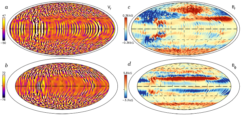
Figure 4: Nests of convection in dynamo case D10L. Convective patterns are shown by snapshots in Mollweide projection of the radial velocities $v_{r}$ $(a)$ near the surface ($0.95\thinspace R_{\odot}$) and $(b)$ at mid-convection zone ($0.85\thinspace R_{\odot}$). Two active nests of convection are clearly visible. $(c)$ Near the surface, the radial magnetic field $B_{r}$ is concentrated in the stronger nest. This patch of radial field propagates with the nest. $(d)$ At mid-convection zone the active nests leave their imprint on the magnetic wreaths, shown here by longitudinal field $B_{\phi}$.

Some of these rapidly rotating dynamos have held further surprises. One such simulation, case D10L rotating ten times faster than the Sun, is shown in Figure 4. Magnetic wreaths form in this dynamo, but so do strong localized nests of convection. Two such nests are visible near the equatorial region in the convective patterns of radial velocity (Fig. 4$a,b$). At certain longitudes the convection is significantly stronger, and these nests span the convection zone. The nests leave their imprint on the magnetism, concentrating the radial magnetic field $B_{r}$ into patches near the surface (Fig. 4$c$) and interacting strongly with the toroidal field $B_{\phi}$ at depth (Fig. 4$d$). These active nests appear to be distinct dynamical structures, and they propagate at a different rate than either individual convective cells or the local differential rotation. If such nests persist in stellar convection zones, they are likely to strongly affect inferences of the global-scale magnetic field. We have found active nests in rapidly rotating hydrodynamic simulations (Brown et al., 2008), but to our knowledge this is the first time such structures have been found in a fully saturated dynamo state.

We have found wreath-like structures in simulations rotating at the solar rotation rate as well (one example appears in the contribution by Miesch, these proceedings). Achieving such structures in solar simulations is challenging, as the angular velocity contrast in the Sun is smaller than that realized in the rapidly rotating dynamos. Generally the solar simulations require low values of $\eta$ to build wreaths, which in turn calls for high resolutions and that exacts a large computational cost.

The magnetic boundary conditions adopted near the base of the convection zone also play an important role: here we have explored simulations with perfectly conducting bottom boundaries. Previous simulations of the solar dynamo (case M3, Brun et al., 2004) used a potential field bottom boundary and did not find magnetic wreaths like those shown here. When the boundary conditions are changed in case M3 to the perfect conducting boundaries used here, the axisymmetric magnetic fields grow in strength, become more organized and form wreaths near the base of the convection zone. A variant on that solar dynamo simulation is shown in the contribution by Miesch in these proceedings. Conversely, magnetic wreaths are difficult to achieve in the rapidly rotating dynamos when we use the boundary conditions of Brun et al. (2004). We take some comfort in the fact that wreaths continue to form in simulations which include a portion of the stable radiative zone within the domain. In the simulations with model tachoclines, the wreaths of magnetism are essentially unmodified from those found in the simulations which only capture the convection zone. This suggests that a perfectly conducting bottom boundary may mimic the presence of a highly-conductive radiative zone below the convection zone better than a potential field extrapolation does.

5 Overview

Stellar convection spans a vast range of spatial and temporal scales which remain well beyond the grasp of direct numerical simulation, and we remain humbled by the complexities posed by highly turbulent convection on global-scales in rotating, stratified, and magnetized plasmas. Stellar dynamo studies must drastically simplify the physics of the stellar interior: as an example, molecular values of $\eta$ in the solar convection zone range from roughly $10^{2}$–$10^{5}\>\mathrm{cm}^{2}/\mathrm{s}$ as one moves from the tachocline to the near surface regions, while the molecular viscosity $\nu$ is of order $10^{\phantom{5}}\mathrm{cm}^{2}/\mathrm{s}$ there. In contrast, our simulations employ values of $\eta$ and $\nu$ that are of order $10^{12}\>\mathrm{cm}^{2}/\mathrm{s}$; this large value is more similar to simple estimates of turbulent diffusion associated with granulation at the surface where $\nu_{\mathrm{t}}\sim V_{\mathrm{t}}L_{\mathrm{t}}\sim 10^{11}\>\mathrm{cm}^{2}/\mathrm{s}$ given $V_{\mathrm{t}}\sim 1\>\mathrm{km}/\mathrm{s}$ and $L_{\mathrm{t}}\sim 1\>\mathrm{Mm}$. Despite this daunting separation in parameter space, it is striking that coherent magnetic structures can arise at all in the midst of turbulent convection. We find the combination of global-scale spatial organization and cyclic behavior fascinating, as these appear to be the first self-consistent 3D convective stellar dynamos to achieve such behavior in the bulk of the convection zone.

A variety of wreath-building dynamos have been found in these simulations of rapidly rotating suns: some build persistent wreaths, while others undergo significant time variations including quasi-cyclic reversals of global-scale magnetic polarity. The parameter space is complex, and some simulations show cycles in one hemisphere but not the other. Cyclic cases like case D5 can even wander into and then back out of non-cycling states. The role of tachoclines in stellar dynamos remains a matter of great debate. These simulations suggest that, at least in rapidly rotating stars, tachoclines may not play as crucial a role in the organization and storage of the global-scale magnetic field as in the solar dynamo. A major step forward will be to explore simulations that couple wreath-building dynamos in the convection zone, through a tachocline of shear, to the stable radiative interior below; those simulations are ongoing now. We are also exploring how convection and dynamo action may be different in other solar-type stars, including K-type dwarfs and the fully convective M-type stars, which present their own mysteries (see Browning, 2008, and contribution by Browning, these proceedings). The future of 3D dynamo simulations is very bright, and cyclic solutions are beginning to appear in a variety of situations (e.g., Ghizaru et al., 2010; Käpylä et al., 2010; Mitra et al., 2010). These are exciting times indeed for stellar dynamo theorists!

This research is supported by NASA through Heliophysics Theory Program grants NNG05G124G and NNX08AI57G, with additional support for Brown through the NASA GSRP program by award number NNG05GN08H and NSF Astronomy and Astrophysics postdoctoral fellowship AST 09-02004. CMSO is supported by NSF grant PHY 08-21899. Miesch was supported by NASA SR&T grant NNH09AK14I. NCAR is sponsored by the National Science Foundation. Browning is supported by research support at CITA. Brun was partly supported by the Programme National Soleil-Terre of CNRS/INSU (France), and by the STARS2 grant from the European Research Council. The simulations were carried out with NSF PACI support of PSC, SDSC, TACC and NCSA.

T. Rogers Could the poleward propagation of field be likened to the dynamo wave, in which the sign of propagation depended on helicity associated with convection versus radiation zones?

B. Brown Maybe. Here we clearly see signs that the poleward propagation is partly due to Maxwell stresses and a resulting poleward slip, and this phenomena occurs essentially unmodified in simulations that include a tachocline and convective penetration into a stable radiative zone. But there may be dynamo wave aspects to the reversals as well. [Note: subsequent work indicates that a non-linear dynamo wave does play an important role in the reversal process; see Brown et al. (2010b).]

E. Zweibel Why is the “failed dynamo” region on the $\eta$–$\Omega$ plane localized near the solar rotation rate ($\Omega=\Omega_{\odot}$)? (see Figure 3$a$)

B. Brown On either side of the solar rotation rate, the latitudinal shear is strong. Simulations spinning slower than the Sun have strong anti-solar differential rotation (retrograde equators, prograde poles) while the more rapidly rotating simulations have stronger solar-like differential rotation (prograde equators, retrograde poles). Both cases lead to higher magnetic Reynolds numbers associated with the latitudinal shear. Simulations at the solar rotation rate have weaker differential rotation, and need lower values of $\eta$ to achieve dynamo action in these wreath-building dynamos.

References

- Brown et al. (2008) Brown, B. P., Browning, M. K., Brun, A. S., Miesch, M. S., & Toomre, J. 2008, ApJ, 689, 1354
- Brown et al. (2010a) —. 2010a, ApJ, 711, 424
- Brown et al. (2010b) Brown, B. P., Miesch, M. S., Browning, M. K., Brun, A. S., & Toomre, J. 2010b, ApJ, submitted
- Browning (2008) Browning, M. K. 2008, ApJ, 676, 1262
- Brun et al. (2004) Brun, A. S., Miesch, M. S., & Toomre, J. 2004, ApJ, 614, 1073
- Clune et al. (1999) Clune, T. L., Elliott, J. R., Glatzmaier, G. A., Miesch, M. S., & Toomre, J. 1999, Parallel Computing, 25, 361
- Ghizaru et al. (2010) Ghizaru, M., Charbonneau, P., & Smolarkiewicz, P. K. 2010, ApJ, 715, L133
- Käpylä et al. (2010) Käpylä, P. J., Korpi, M. J., Brandenburg, A., Mitra, D., & Tavakol, R. 2010, Astronomische Nachrichten, 331, 73
- Miesch et al. (2000) Miesch, M. S., Elliott, J. R., Toomre, J., Clune, T. L., Glatzmaier, G. A., & Gilman, P. A. 2000, ApJ, 532, 593
- Mitra et al. (2010) Mitra, D., Tavakol, R., Käpylä, P. J., & Brandenburg, A. 2010, ApJ, 719, L1
- Pizzolato et al. (2003) Pizzolato, N., Maggio, A., Micela, G., Sciortino, S., & Ventura, P. 2003, A&A, 397, 147