Introduction to a Quantum Theory over a Galois Field

Felix M. Lev

Artwork Conversion Software Inc., 1201 Morningside Drive, Manhattan Beach, CA 90266, USA (Email: felixlev314@gmail.com)

Abstract:

We consider a quantum theory based on a Galois field. In this approach infinities cannot exist, the cosmological constant problem does not arise, and one irreducible representation (IR) of the symmetry algebra splits into independent IRs describing a particle an its antiparticle only in the approximation when de Sitter energies are much less than the characteristic of the field. As a consequence, the very notions of particles and antiparticles are only approximate and such additive quantum numbers as the electric, baryon and lepton charges are conserved only in this approximation. There can be no neutral elementary particles and the spin-statistics theorem can be treated simply as a requirement that standard quantum theory should be based on complex numbers.

Key words: quantum theory; Galois fields; elementary particles

PACS: 02.10.De, 03.65.Ta, 11.30.Fs, 11.30.Ly

1 Motivation

The most striking feature of the modern quantum theory is probably the following. On one hand, this theory describes many experimental data with an unprecedented accuracy. On the other hand, the mathematical substantiation of the theory is rather poor. As a consequence, the issue of infinities is probably the most challenging problem in standard formulation of quantum theory. As noted by Weinberg [1], “Disappointingly this problem appeared with even greater severity in the early days of quantum theory, and although greatly ameliorated by subsequent improvements in the theory, it remains with us to the present day”. While in QED and other renormalizable theories infinities can be somehow circumvented, in quantum gravity this is not possible even in lowest orders of perturbation theory. A recent Weinberg’s paper [2] is entitled “Living with Infinities”.

Mathematical problems of quantum theory are discussed in a wide literature. For example, in the well known textbook [3] it is explained in details that interacting quantized fields can be treated only as operatorial distributions and hence their product at the same point is not well defined. One of ideas of the string theory is that if a point (a zero-dimensional object) is replaced by a string (a one-dimensional object) then there is a hope that infinities will be less singular.

There exists a wide literature aiming to solve the difficulties of the theory by replacing the field of complex numbers by quaternions, p-adic numbers or other constructions. For example, a detailed description of a quaternionic theory is given in a book [4] and a modern state-of-the-art of the p-adic theory can be found, for example, in Reference [5]. At present it is not clear how to overcome all the difficulties but at least from the point of view of the problem of infinities a natural approach is to consider a quantum theory over Galois fields (GFQT). Since any Galois field is finite, the problem of infinities in GFQT does not exist in principle and all operators are well defined. The idea of using finite fields in quantum theory has been discussed by several authors (see e.g., References [6, 7, 8, 9, 10, 11, 12]). As stated in Reference [12], a fundamental theory can be based either on p-adic numbers or finite fields. In that case, a correspondence with standard theory will take place if the number $p$ in the p-adic theory or as a characteristic of a finite field is rather large.

The authors of Reference [12] and many other papers argue that fundamental quantum theory cannot be based on mathematics using standard geometrical objects (such as strings, branes, etc.) at Planck distances. We believe it is rather obvious that the notions of continuity, differentiability, smooth manifolds etc. are based on our macroscopic experience. For example, the water in the ocean can be described by equations of hydrodynamics but we know that this is only an approximation since matter is discrete. Therefore continuous geometry probably does not describe physics even at distances much greater than the Planck length (also see the discussion below).

In our opinion an approach based on finite fields is very attractive for solving problems in quantum theory as well as for philosophical and aesthetical reasons. Below we describe some arguments in favor of this opinion.

The key ingredient of standard mathematics is the notions of infinitely small and infinitely large numbers. The notion of infinitely small numbers is based on our everyday experience that any macroscopic object can be divided by two, three and even a million parts. But is it possible to divide by two or three the electron or neutrino? It is obvious that if elementary particles exist, then division has only a limited meaning. Indeed, consider, for example, the gram-molecule of water having the mass 18 grams. It contains the Avogadro number of molecules $6\cdot 10^{23}$. We can divide this gram-molecule by ten, million, etc., but when we begin to divide by numbers greater than the Avogadro one, the division operation loses its sense. The conclusion is that if we accept the existence of elementary particles, we should acknowledge that our experience based on standard mathematics is not universal.

The notion of infinitely large numbers is based on the belief that in principle we can operate with any large numbers. In standard mathematics this belief is formalized in terms of axioms (accepted without proof) about infinite sets (e.g., Zorn’s lemma or Zermelo’s axiom of choice). At the same time, in the spirit of quantum theory, there should be no statements accepted without proof since only those statements have physical significance, which can be experimentally verified, at least in principle.

For example, we cannot verify that $a+b=b+a$ for any numbers $a$ and $b$. Suppose we wish to verify that 100+200=200+100. In the spirit of quantum theory, it is insufficient to say that 100+200=300 and 200+100=300. To check these relationships, we should describe an experiment where they can be verified. In particular, we should specify whether we have enough resources to represent the numbers 100, 200 and 300. We believe the following observation is very important: although standard mathematics is a part of our everyday life, people typically do not realize that standard mathematics is implicitly based on the assumption that one can have any desirable amount of resources.

A well known example in standard mathematics is that the interval $(0,1)$ has the same cardinality as $(-\infty,\infty)$. Another example is that the function $tgx$ gives a one-to-one relation between the intervals $(-\pi/2,\pi/2)$ and $(-\infty,\infty)$. Therefore one can say that a part has the same number of elements as a whole. One might think that this contradicts common sense but in standard mathematics the above facts are not treated as contradicting. Self-consistency of standard mathematics has been discussed by numerous authors. For example, the famous Goedel’s incompleteness theorems are interpreted as showing that Hilbert’s program to find a complete and consistent set of axioms for all of mathematics is impossible.

Suppose now that our Universe is finite and contains only a finite number of elementary particles. This implies that the amount of resources cannot be infinite and the rules of arithmetic such as $a+b=b+a$ for any numbers $a$ and $b$, cannot be verified in principle. In this case it is natural to assume that there exists a number $p$ such that all calculations can be performed only modulo $p$. Note that for any system with a finite amount of resources, the only way of performing self-consistent calculations is to perform them modulo some number. One might consider a quantum theory over a Galois field with the characteristic $p$. Since any Galois field is finite, the fact that arithmetic in this field is correct can be verified, at least in principle, by using a finite amount of resources. Note that the proofs of the Goedel incompleteness theorems are based on the fact that standard arithmetic is infinite but in our case no inconsistencies arise.

The example with division might be an indication that, in the spirit of Reference [13], the ultimate quantum theory will be based even not on a Galois field but on a finite ring (this observation was pointed out to me by Metod Saniga). However, in the present paper we will consider a case of Galois fields.

If one accepts the idea to replace complex numbers by a Galois field, the problem arises what formulation of standard quantum theory is most convenient for that purpose. A well known historical fact is that originally quantum theory has been proposed in two formalisms which seemed essentially different: the Schroedinger wave formalism and the Heisenberg operator (matrix) formalism. It has been shown later by Born, von Neumann and others that both formalisms are equivalent and, in addition, the path integral formalism has been developed.

In the spirit of the wave or path integral approach one might try to replace classical spacetime by a finite lattice which may even not be a field. In that case the problem arises what the natural “quantum of spacetime” is and some of physical quantities should necessarily have the field structure. A detailed discussion can be found in Reference [6, 7, 8, 9, 10, 11] and references therein. In contrast to these approaches, we propose to generalize the standard operator formulation, where quantum systems are described by elements of a projective complex Hilbert spaces and physical quantities are represented by self-adjoint operators in such spaces.

From the point of view of quantum theory, any physical quantity can be discussed only in conjunction with the operator defining this quantity. However, in textbooks on quantum mechanics it is usually not indicated explicitly that the quantity $t$ is a parameter, which has the meaning of time only in the classical limit since there is no operator corresponding to this quantity. The problem of how time should be defined on quantum level is very difficult and is discussed in a vast literature (see e.g., References [16, 17, 18] and references therein). Since the 1930’s it has been well known [19] that, when quantum mechanics is combined with relativity, there is no operator satisfying all the properties of the spatial position operator. In other words, the coordinate cannot be exactly measured even in situations when exact measurement is allowed by the non-relativistic uncertainty principle. In the introductory section of the well-known textbook [20] simple arguments are given that for a particle with mass $m$, the coordinate cannot be measured with the accuracy better than the Compton wave length ${\hbar}/mc$. Hence, the exact measurement is possible only either in the non-relativistic limit (when $c\to\infty$) or classical limit (when ${\hbar}\to 0)$. From the point of view of quantum theory, one can discuss if the coordinates of particles can be measured with a sufficient accuracy, while the notion of empty spacetime background fully contradicts basic principles of this theory. Indeed, the coordinates of points, which exist only in our imagination are not measurable and this problem has been discussed in a wide literature (see e.g., References [16, 17, 18, 21]). In particular, the quantity $x$ in the Lagrangian density $L(x)$ is not measurable. Note that Lagrangian is only an auxiliary tool for constructing Hilbert spaces and operators and this is all we need to have the maximum possible information in quantum theory. After this construction has been done, one can safely forget about Lagrangian and concentrate his or her efforts on calculating different observables. As stated in Reference [20], local quantum fields and Lagrangians are rudimentary notion, which will disappear in the ultimate quantum theory. Analogous ideas were the basis of the Heisenberg S-matrix program.

In view of the above discussion, we define GFQT as a theory where

• Quantum states are represented by elements of a linear projective space over a Galois field and physical quantities are represented by linear operators in that space.

As noted in Reference [5] and references therein, in the p-adic theory a problem arises what number fields are preferable and there should be quantum fluctuations not only of metrics and geometry but also of the number field. Volovich [12] proposed the following number field invariance principle: fundamental physical laws should be invariant under the change of the number field. Analogous questions can be posed in GFQT.

It is well known (see, e.g., standard textbooks [22, 23, 24]) that any Galois field can contain only $p^{n}$ elements where $p$ is prime and $n$ is natural. Moreover, the numbers $p$ and $n$ define the Galois field up to isomorphism. It is natural to require that there should exist a correspondence between any new theory and the old one, i.e., at some conditions both theories should give close predictions. In particular, there should exist a large number of quantum states for which the probabilistic interpretation is valid. Then, as shown in our papers [25, 26, 27], in agreement with References [6, 7, 8, 9, 10, 11, 12], the number $p$ should be very large. Hence, we have to understand whether there exist deep reasons for choosing a particular value of $p$ or it is simply an accident that our Universe has been created with this value. Since we don’t know the answer, we accept a simplest version of GFQT, where there exists only one Galois field with the characteristic $p$, which is a universal constant for our Universe. Then the problem arises what the value of $n$ is. Since there should exist a correspondence between GFQT and the complex version of standard quantum theory, a natural idea is to accept that the principal number field in GFQT is the Galois field analog of complex numbers which is constructed below.

Let $F_{p}=Z/pZ$ be a residue field modulo $p$ and $F_{p^{2}}$ be a set of $p^{2}$ elements $a+bi$ where $a,b\in F_{p}$ and $i$ is a formal element such that $i^{2}=-1$. The question arises whether $F_{p^{2}}$ is a field, i.e., one can define all the arithmetic operations except division by zero. The definition of addition, subtraction and multiplication in $F_{p^{2}}$ is obvious and, by analogy with the field of complex numbers, one could define division as $1/(a+bi)\,=a/(a^{2}+b^{2})\,-ib/(a^{2}+b^{2})$ if $a$ and $b$ are not equal to zero simultaneously. This definition can be meaningful only if $a^{2}+b^{2}\neq 0$ in $F_{p}$. If $a$ and $b$ are not simultaneously equal to zero, this condition can obviously be reformulated such that $-1$ should not be a square in $F_{p}$ (or in terminology of number theory it should not be a quadratic residue). We will not consider the case $p=2$ and then $p$ is necessarily odd. Then we have two possibilities: the value of $p\,(mod\,4)$ is either 1 or 3. The well known result of number theory is that -1 is a quadratic residue only in the former case and a quadratic non-residue in the latter one, which implies that the above construction of the field $F_{p^{2}}$ is correct only if $p=3\,\,(mod\,4)$.

The main idea of establishing the correspondence between GFQT and standard theory is as follows (see References [25, 26, 27] for a detailed discussion). The first step is to notice that the elements of $F_{p}$ can be written not only as $0,1,...p-1$ but also as $0,\pm 1,...,\pm(p-1)/2$. Such elements of $F_{p}$ are called minimal residues [22, 23, 24]. Since the field $F_{p}$ is cyclic, it is convenient to visually depict its elements by the points of a circumference of the radius $p/2\pi$ on the plane $(x,y)$ such that the distance between neighboring elements of the field is equal to unity and the elements 0, 1, 2,… are situated on the circumference counterclockwise. At the same time we depict the elements of $Z$ as usual, such that each element $z\in Z$ is depicted by a point with the coordinates $(z,0)$. In Fig. 1 a part of the circumference near the origin is depicted.

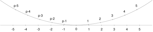
Figure 1: Relation between $F_{p}$ and the ring of integers.

Let $f$ be a map from $F_{p}$ to $Z$ such that $f(a)$ has the same notation in $Z$ as its minimal residue in $F_{p}$. Then for elements $a,b\in F_{p}$ such that $|f(a)|,|f(b)|\ll p$, addition, subtraction and multiplication in $F_{p}$ and $Z$ are the same, i.e., $f(a\pm b)=f(a)\pm f(b)$ and $f(ab)=f(a)f(b)$.

The second step is to establish a correspondence between Hilbert spaces in standard theory and spaces over a Galois field in GFQT. We first note that the Hilbert space $H$ contains a big redundancy of elements and we do not need to know all of them. Since a set of finite linear combinations of basis elements with rational coefficients is dense in $H$, with any desired accuracy we can approximate each element $\tilde{x}$ from $H$ by a finite linear combination $\tilde{x}=\tilde{c}_{1}\tilde{e}_{1}+\tilde{c}_{2}\tilde{e}_{2}+...\tilde{c}_{n}\tilde{e}_{n}$ where $(\tilde{c}_{1},\tilde{c}_{2},...\tilde{c}_{n})$ are rational complex numbers. In turn, the set of such elements is redundant too. We can use the fact that Hilbert spaces in quantum theory are projective: $\psi$ and $c\psi$ represent the same physical state, which reflects the fact that not the probability itself but the relative probabilities of different measurement outcomes have a physical meaning. Therefore we can multiply both parts of the above equality by a common denominator of the numbers $(\tilde{c}_{1},\tilde{c}_{2},...\tilde{c}_{n})$. As a result, we can always assume that $\tilde{c}_{j}=\tilde{a}_{j}+i\tilde{b}_{j}$ where $\tilde{a}_{j}$ and $\tilde{b}_{j}$ are integers.

Consider now a space over $F_{p^{2}}$ and let $x=c_{1}e_{1}+c_{2}e_{2}+...c_{n}e_{n}$ be a decomposition of a state $x$ over a basis $(e_{1},e_{2}...)$ in this space. We can formally define a scalar product $(e_{j},e_{k})$ such that $f((e_{j},e_{k}))=(\tilde{e}_{j},\tilde{e}_{k})$. Then the correspondence between the states $x$ and ${\tilde{x}}$ can be defined such that $c_{j}=a_{j}+ib_{j}$ $(j=1,2...)$, $f(a_{j})=\tilde{a}_{j}$ and $f(b_{j})=\tilde{b}_{j}$. If the numbers in question are much less than $p$ then the standard description and that based on GFQT give close experimental predictions. At the same time, in GFQT a probabilistic interpretation is not universal and is valid only when the numbers in question are much less than $p$.

The above discussion has a well known historical analogy. For many years people believed that our Earth was flat and infinite, and only after a long period of time they realized that it was finite and had a curvature. It is difficult to notice the curvature when we deal only with distances much less than the radius of the curvature $R$. Analogously one might think that the set of numbers describing physics has a curvature defined by a very large number $p$ but we do not notice it when we deal only with numbers much less than $p$.

Since we treat GFQT as a more general theory than standard one, it is desirable not to postulate that GFQT is based on $F_{p^{2}}$ (with $p=3\,\,(mod\,4)$) because standard theory is based on complex numbers but vice versa, explain the fact that standard theory is based on complex numbers since GFQT is based on $F_{p^{2}}$. Hence, one should find a motivation for the choice of $F_{p^{2}}$ in GFQT. A possible motivation is discussed in References [27, 28] and in Section 10 of the present paper.

In standard approach to symmetries in quantum theory, the symmetry group is a group of motions of a classical spacetime background. As noted above, in quantum theory the spacetime background does not have a physical meaning. So a question arises whether there exists an alternative for such an approach. As already noted, in standard approach, the spacetime background and Lagrangian are only auxiliary tools for constructing Hilbert spaces and operators. For calculating observables one needs not representation operators of the symmetry group but representation operators of its Lie algebra, e.g., the Hamiltonian. The representation operators of the group are needed only if it is necessary to calculate macroscopic transformations, e.g., spacetime transformations. In the approximation when classical time and space are good approximate parameters, the Hamiltonian and momentum operators can be interpreted as ones associated with the corresponding translations, but nothing guarantees that this interpretation is always valid (e.g., at the very early stage of the Universe). One might think that this observation is not very significant, since typically symmetry groups are Lie groups and for them in many cases there exits a one-to-one correspondence between representations of the Lie group and its Lie algebra. However, in Galois fields there is no notion of infinitesimal transformations and hence there is no notion of Lie group over a Galois field associated with a given Lie algebra over a Galois field.

Each system is described by a set of independent operators and they somehow commute with each other. By definition, the rules how they commute define a Lie algebra which is treated as a symmetry algebra. Such a definition of symmetry on quantum level is in the spirit of Dirac’s paper [29]. We believe that for understanding this Dirac’s idea the following example might be useful. If we define how the energy should be measured (e.g., the energy of bound states, kinetic energy etc.), we have a full knowledge about the Hamiltonian of our system. In particular, we know how the Hamiltonian should commute with other operators. In standard theory the Hamiltonian is also interpreted as an operator responsible for evolution in time, which is considered as a classical macroscopic parameter. According to principles of quantum theory, self-adjoint operators in Hilbert spaces represent observables but there is no requirement that parameters defining a family of unitary transformations generated by a self-adjoint operator are eigenvalues of another self-adjoint operator. A well known example from standard quantum mechanics is that if $P_{x}$ is the $x$ component of the momentum operator then the family of unitary transformations generated by $P_{x}$ is $exp(iP_{x}x/\hbar)$ where $x\in(-\infty,\infty)$ and such parameters can be identified with the spectrum of the position operator. At the same time, the family of unitary transformations generated by the Hamiltonian $H$ is $exp(-iHt/\hbar)$ where $t\in(-\infty,\infty)$ and those parameters cannot be identified with a spectrum of a self-adjoint operator on the Hilbert space of our system. In the relativistic case the parameters $x$ can be formally identified with the spectrum of the Newton-Wigner position operator [19] but it is well known that this operator does not have all the required properties for the position operator. So, although the operators $exp(iP_{x}x/\hbar)$ and $exp(-iHt/\hbar)$ are well defined in standard theory, their physical interpretation as translations in space and time is not always valid.

Let us now discuss how one should define the notion of elementary particles. Although particles are observables and fields are not, in the spirit of quantum field theory (QFT), fields are more fundamental than particles, and a possible definition is as follows [30]: It is simply a particle whose field appears in the Lagrangian. It does not matter if it’s stable, unstable, heavy, light—if its field appears in the Lagrangian then it’s elementary, otherwise it’s composite. Another approach has been developed by Wigner in his investigations of unitary irreducible representations (IRs) of the Poincare group [31]. In view of this approach, one might postulate that a particle is elementary if the set of its wave functions is the space of a unitary IR of the symmetry group or Lie algebra in the given theory. In standard theory the Lie algebras are usually real and one considers their representations in complex Hilbert spaces.

In view of the above remarks, and by analogy with standard quantum theory one might define the elementary particle in GFQT as follows. Let ${\cal A}$ be a Lie algebra over $F_{p}$ which is treated as a symmetry algebra. A particle is elementary if the set of its states forms an IR of ${\cal A}$ in $F(p^{n})$. Representations of Lie algebras in spaces with nonzero characteristic are called modular representations. There exists a well developed theory of such representations. One of the well known results is the Zassenhaus theorem [32] that any modular IR is finite dimensional. In Section 6 we propose another definition of elementary particle.

As argued in References [25, 26, 27], standard theories based on de Sitter (dS) algebra so(1,4) or anti de Sitter (AdS) algebra so(2,3) can be generalized to theories based on a Galois field while there are problems with the generalization of the theory based on Poincare algebra. The reasons are the following. It is clear that in theories based on Galois fields there can be no dimensional quantities and all physical quantities are discrete. In standard dS or AdS invariant theories all physical quantities are dimensionless and discrete in units $\hbar/2=c=1$ while in Poincare invariant theory the energy and momentum necessarily have a continuous spectrum. From the formal point of view, the representation operators of the Poincare algebra can also be chosen dimensionless, e.g., in Planck units. In Poincare invariant theories over a Galois field one has to choose a quantum of length. If this quantum is the Planck distance then the quantum of mass will be the Planck mass, which is much greater than the masses of elementary particles.

The existing astronomical data (see, e.g., Reference [33, 34]) indicate that the cosmological constant is small and positive. This is an argument in favor of so(1,4) vs. so(2,3). On the other hand, in QFT and its generalizations (string theory, M-theory etc.) a theory based on so(1,4) encounters serious difficulties and the choice of so(2,3) is preferable (see e.g., Reference [35]). IRs of the so(2,3) algebra have much in common with IRs of Poincare algebra. In particular, in IRs of the so(2,3) algebra the AdS Hamiltonian is either strictly positive or strictly negative and a supersymmetric generalization is possible. In standard theory, representations of the so(2,3) and so(1,4) algebras differ only in a way how Hermiticity conditions are imposed. Since in GFQT the notions of probability and Hermiticity are only approximate, modular representations of those algebras differ only in a way how we establish a correspondence with standard theory when $p$ is large. For these reasons in the present paper for illustration of what happens when complex numbers are replaced by a Galois field we assume that ${\cal A}$ is the modular analog of the algebra so(2,3).

It is well known [22, 23, 24] that the field $F_{p^{n}}$ has $n-1$ nontrivial automorphisms. Therefore, if $n$ is arbitrary, a formal scalar product and Hermiticity can be defined in different ways. We do not assume from the beginning that $n=2$ and $p=3\,\,(mod\,4)$. Our results do not depend on the explicit choice of the scalar product and ${\bar{z}}$ is used to denote an element obtained from $z\in F_{p^{n}}$ by an automorphism compatible with the scalar product in question.

The paper is organized as follows. In Sections 2-4 we construct modular IRs describing elementary particles in GFQT, their quantization and physical meaning are discussed in Sections 5-9, the spin-statistics theorem is discussed in Section 10 and a supersymmetric generalization is discussed in Section 11. Although some results require extensive calculations, they involve only finite sums in Galois fields. For this reason all the results can be reproduced even by readers who previously did not have practice in calculations with Galois fields. A more detailed description of calculations can be found in Reference [27].

2 Modular IRs of the sp(2) Algebra

The key role in constructing modular IRs of the so(2,3) algebra is played by modular IRs of the sp(2) subalgebra. They are described by a set of operators $(a^{\prime},a",h)$ satisfying the commutation relations

$$[h,a^{\prime}]=-2a^{\prime}\quad[h,a"]=2a"\quad[a^{\prime},a"]=h$$ (1)

The Casimir operator of the second order for the algebra (1) has the form

$$K=h^{2}-2h-4a"a^{\prime}=h^{2}+2h-4a^{\prime}a"$$ (2)

We first consider representations with the vector $e_{0}$ such that

$$a^{\prime}e_{0}=0,\quad he_{0}=q_{0}e_{0}$$ (3)

where $q_{0}\in F_{p}$ and $f(q_{0})>0$. Recall that we consider the representation in a linear space over $F_{p^{k}}$ where $k$ is a natural number (see the discussion in Section 1). Denote $e_{n}=(a")^{n}e_{0}$. Then it follows from Equations (2) and (3), that

$$he_{n}=(q_{0}+2n)e_{n},\quad Ke_{n}=q_{0}(q_{0}-2)e_{n}$$ (4)

$$a^{\prime}a"e_{n}=(n+1)(q_{0}+n)e_{n}$$ (5)

One can consider analogous representations in standard theory. Then $q_{0}$ is a positive real number, $n=0,1,2,...$ and the elements $e_{n}$ form a basis of the IR. In this case $e_{0}$ is a vector with a minimum eigenvalue of the operator $h$ (minimum weight) and there are no vectors with the maximum weight. The operator $h$ is positive definite and bounded below by the quantity $q_{0}$. For these reasons the above modular IRs can be treated as modular analogs of such standard IRs that $h$ is positive definite.

Analogously, one can construct modular IRs starting from the element $e_{0}^{\prime}$ such that

$$a"e_{0}^{\prime}=0,\quad he_{0}^{\prime}=-q_{0}e_{0}^{\prime}$$ (6)

and the elements $e_{n}^{\prime}$ can be defined as $e_{n}^{\prime}=(a^{\prime})^{n}e_{0}^{\prime}$. Such modular IRs are analogs of standard IRs where $h$ is negative definite. However, in the modular case Equations (3) and (6) define the same IRs. This is clear from the following consideration.

The set $(e_{0},e_{1},...e_{N})$ will be a basis of IR if $a"e_{i}\neq 0$ for $i<N$ and $a"e_{N}=0$. These conditions must be compatible with $a^{\prime}a"e_{N}=0$. Therefore, as follows from Equation (5), $N$ is defined by the condition $q_{0}+N=0$ in $F_{p}$. As a result, if $q_{0}$ is one of the numbers $1,...p-1$ then $N=p-q_{0}$ and the dimension of IR equals $p-q_{0}+1$ (in agreement with the Zassenhaus theorem [32]). It is easy to see that $e_{N}$ satisfies Equation (6) and therefore it can be identified with $e_{0}^{\prime}$.

Let us forget for a moment that the eigenvalues of the operator $h$ belong to $F_{p}$ and will treat them as integers. Then, as follows from Equation (4), the eigenvalues are

$$q_{0},q_{0}+2,...,2p-2-q_{0},2p-q_{0}.$$

Therefore, if $f(q_{0})>0$ and $f(q_{0})\ll p$, the maximum value of $q_{0}$ is equal to $2p-q_{0}$, i.e., it is of order $2p$.

3 Modular IRs of the so(2,3) Algebra

Standard IRs of the so(2,3) algebra relevant for describing elementary particles have been considered by several authors. The description in this section is a combination of two elegant ones given in Reference [36] for standard IRs and Reference [37] for modular IRs. In standard theory, the commutation relations between the representation operators in units $\hbar/2=c=1$ are given by

$$[M^{ab},M^{cd}]=-2i(g^{ac}M^{bd}+g^{bd}M^{cd}-g^{ad}M^{bc}-g^{bc}M^{ad})$$ (7)

where $a,b,c,d$ take the values 0,1,2,3,5 and the operators $M^{ab}$ are antisymmetric. The diagonal metric tensor has the components $g^{00}=g^{55}=-g^{11}=-g^{22}=-g^{33}=1$. In these units the spin of fermions is odd, and the spin of bosons is even. If $s$ is the particle spin then the corresponding IR of the su(2) algebra has the dimension $s+1$.

Note that our definition of the AdS symmetry on quantum level does not involve the cosmological constant at all. It appears only if one is interested in interpreting results in terms of the AdS spacetime or in the Poincare limit. Since all the operators $M^{ab}$ are dimensionless in units $\hbar/2=c=1$, the de Sitter invariant quantum theories can be formulated only in terms of dimensionless variables. As noted in Section 1, this is a necessary requirement for a theory, which is supposed to have a physical generalization to the case of Galois fields. At the same time, since Poincare invariant theories do not have such generalizations, one might expect that quantities which are dimensionful in units $\hbar/2=c=1$ are not fundamental. This is in the spirit of Mirmovich’s hypothesis [38] that only quantities having the dimension of the angular momentum can be fundamental.

If a modular IR is considered in a linear space over $F_{p^{2}}$ with $p=3\,\,(mod\,\,4)$ then Equation (7) is also valid. However, as noted in Section 1, we consider modular IRs in linear spaces over $F_{p^{k}}$ where $k$ is arbitrary. In this case it is convenient to work with another set of ten operators. Let $(a_{j}^{\prime},a_{j}",h_{j})$ $(j=1,2)$ be two independent sets of operators satisfying the commutation relations for the sp(2) algebra

$$[h_{j},a_{j}^{\prime}]=-2a_{j}^{\prime}\quad[h_{j},a_{j}"]=2a_{j}"\quad[a_{j}^{\prime},a_{j}"]=h_{j}$$ (8)

The sets are independent in the sense that for different $j$ they mutually commute with each other. We denote additional four operators as $b^{\prime},b",L_{+},L_{-}$. The operators $L_{3}=h_{1}-h_{2},L_{+},L_{-}$ satisfy the commutation relations of the su(2) algebra

$$[L_{3},L_{+}]=2L_{+}\quad[L_{3},L_{-}]=-2L_{-}\quad[L_{+},L_{-}]=L_{3}$$ (9)

while the other commutation relations are as follows

$$[a_{1}^{\prime},b^{\prime}]=[a_{2}^{\prime},b^{\prime}]=[a_{1}",b"]=[a_{2}",b"]=[a_{1}^{\prime},L_{-}]=[a_{1}",L_{+}]=[a_{2}^{\prime},L_{+}]=$$

$$[a_{2}",L_{-}]=0\quad[h_{j},b^{\prime}]=-b^{\prime}\quad[h_{j},b"]=b"\quad[h_{1},L_{\pm}]=\pm L_{\pm}\quad[h_{2},L_{\pm}]=\mp L_{\pm}$$

$$[b^{\prime},b"]=h_{1}+h_{2}\quad[b^{\prime},L_{-}]=2a_{1}^{\prime}\quad[b^{\prime},L_{+}]=2a_{2}^{\prime}\quad[b",L_{-}]=-2a_{2}"$$

$$[b",L_{+}]=-2a_{1}"\quad[a_{1}^{\prime},b"]=[b^{\prime},a_{2}"]=L_{-}\quad[a_{2}^{\prime},b"]=[b^{\prime},a_{1}"]=L_{+}$$

$$[a_{1}^{\prime},L_{+}]=[a_{2}^{\prime},L_{-}]=b^{\prime}\quad[a_{2}",L_{+}]=[a_{1}",L_{-}]=-b"$$ (10)

At first glance these relations might seem rather chaotic but in fact they are very natural in the Weyl basis of the so(2,3) algebra.

In spaces over $F_{p^{2}}$ with $p=3\,\,(mod\,\,4)$ the relation between the above sets of ten operators is

$$M_{10}=i(a_{1}"-a_{1}^{\prime}-a_{2}"+a_{2}^{\prime})\quad M_{15}=a_{2}"+a_{2}^{\prime}-a_{1}"-a_{1}^{\prime}$$

$$M_{20}=a_{1}"+a_{2}"+a_{1}^{\prime}+a_{2}^{\prime}\quad M_{25}=i(a_{1}"+a_{2}"-a_{1}^{\prime}-a_{2}^{\prime})$$

$$M_{12}=L_{3}\quad M_{23}=L_{+}+L_{-}\quad M_{31}=-i(L_{+}-L_{-})$$

$$M_{05}=h_{1}+h_{2}\quad M_{35}=b^{\prime}+b"\quad M_{30}=-i(b"-b^{\prime})$$ (11)

and therefore the sets are equivalent. However, the relations (8-10) are more general since they can be used when the representation space is a space over $F_{p^{k}}$ with an arbitrary $k$.

We use the basis in which the operators $(h_{j},K_{j})$ $(j=1,2)$ are diagonal. Here $K_{j}$ is the Casimir operator (2) for algebra $(a_{j}^{\prime},a_{j}",h_{j})$. For constructing IRs we need operators relating different representations of the sp(2)$\times$sp(2) algebra. By analogy with References [36, 37], one of the possible choices is as follows

$$A^{++}=b"(h_{1}-1)(h_{2}-1)-a_{1}"L_{-}(h_{2}-1)-a_{2}"L_{+}(h_{1}-1)+a_{1}"a_{2}"b^{\prime}$$

$$A^{+-}=L_{+}(h_{1}-1)-a_{1}"b^{\prime}\quad A^{-+}=L_{-}(h_{2}-1)-a_{2}"b^{\prime}\quad A^{--}=b^{\prime}$$ (12)

We consider the action of these operators only on the space of minimal sp(2)$\times$sp(2) vectors, i.e., such vectors $x$ that $a_{j}^{\prime}x=0$ for $j=1,2$, and $x$ is the eigenvector of the operators $h_{j}$. If $x$ is a minimal vector such that $h_{j}x=\alpha_{j}x$ then $A^{++}x$ is the minimal eigenvector of the operators $h_{j}$ with the eigenvalues $\alpha_{j}+1$, $A^{+-}x$ - with the eigenvalues $(\alpha_{1}+1,\alpha_{2}-1)$, $A^{-+}x$ - with the eigenvalues $(\alpha_{1}-1,\alpha_{2}+1)$, and $A^{--}x$ - with the eigenvalues $\alpha_{j}-1$.

By analogy with References [36, 37], we require the existence of the vector $e_{0}$ satisfying the conditions

$$a_{j}^{\prime}e_{0}=b^{\prime}e_{0}=L_{+}e_{0}=0\quad h_{j}e_{0}=q_{j}e_{0}\quad(j=1,2)$$ (13)

where $q_{j}\in F_{p}$, $f(q_{j})>0$ for $j=1,2$ and $f(q_{1}-q_{2})\geq 0$. It is well known (see e.g., Reference [27]) that $M^{05}=h_{1}+h_{2}$ is the AdS analog of the energy operator. As follows from Equations (8) and (10), the operators $(a_{1}^{\prime},a_{2}^{\prime},b^{\prime})$ reduce the AdS energy by two units. Therefore $e_{0}$ is an analog the state with the minimum energy which can be called the rest state, and the spin in our units is equal to the maximum value of the operator $L_{3}=h_{1}-h_{2}$ in that state. For these reasons we use $s$ to denote $q_{1}-q_{2}$ and $m$ to denote $q_{1}+q_{2}$. In standard classification [36], the massive case is characterized by the condition $q_{2}>1$ and the massless one—by the condition $q_{2}=1$. There also exist two exceptional IRs discovered by Dirac [39] (Dirac singletons). They are characterized by the conditions $m=1,\,\,s=0$ and $m=2,\,\,s=1$. In this section we will consider the massive case while the singleton and massless cases will be considered in the next section.

As follows from the above remarks, the elements

$$e_{nk}=(A^{++})^{n}(A^{-+})^{k}e_{0}$$ (14)

represent the minimal sp(2)$\times$sp(2) vectors with the eigenvalues of the operators $h_{1}$ and $h_{2}$ equal to $Q_{1}(n,k)=q_{1}+n-k$ and $Q_{2}(n,k)=q_{2}+n+k$, respectively. It can be shown by a direct calculation that

$$A^{--}A^{++}e_{nk}=(n+1)(m+n-2)(q_{1}+n)(q_{2}+n-1)e_{nk}$$ (15)

$$A^{+-}A^{-+}e_{nk}=(k+1)(s-k)(q_{1}-k-2)(q_{2}+k-1)e_{nk}$$ (16)

As follows from these expressions, in the massive case $k$ can assume only the values $0,1,...s$ and in standard theory $n=0,1,...\infty$. However, in the modular case $n=0,1,...n_{max}$ where $n_{max}$ is the first number for which the r.h.s. of Equations (15) becomes zero in $F_{p}$. Therefore $n_{max}=p+2-m$.

The full basis of the representation space can be chosen in the form

$$e(n_{1}n_{2}nk)=(a_{1}")^{n_{1}}(a_{2}")^{n_{2}}e_{nk}$$ (17)

In standard theory $n_{1}$ and $n_{2}$ can be any natural numbers. However, as follows from the results of the preceding section, Equation (8) and the properties of the $A$ operators,

$$n_{1}=0,1,...N_{1}(n,k)\quad n_{2}=0,1,...N_{2}(n,k)$$

$$N_{1}(n,k)=p-q_{1}-n+k\quad N_{2}(n,k)=p-q_{2}-n-k$$ (18)

As a consequence, the representation is finite dimensional in agreement with the Zassenhaus theorem [32] (moreover, it is finite since any Galois field is finite).

Let us assume additionally that the representation space is supplied by a scalar product (see Section 1). The element $e_{0}$ can always be chosen such that $(e_{0},e_{0})=1$. Suppose that the representation operators satisfy the Hermiticity conditions $L_{+}^{*}=L_{-}$, $a_{j}^{{}^{\prime}*}=a_{j}"$, $b^{{}^{\prime}*}=b"$ and $h_{j}^{*}=h_{j}$. Then, as follows from Equation (11), in a special case when the representation space is a space over $F_{p^{2}}$ with $p=3\,\,(mod\,\,4)$, the operators $M^{ab}$ are Hermitian as it should be. By using Equations (8-16), one can show by a direct calculation that the elements $e(n_{1}n_{2}nk)$ are mutually orthogonal while the quantity

$$Norm(n_{1}n_{2}nk)=(e(n_{1}n_{2}nk),e(n_{1}n_{2}nk))$$ (19)

can be represented as

$$Norm(n_{1}n_{2}nk)=F(n_{1}n_{2}nk)G(nk)$$ (20)

where

$$F(n_{1}n_{2}nk)=n_{1}!(Q_{1}(n,k)+n_{1}-1)!n_{2}!(Q_{2}(n,k)+n_{2}-1)!$$

$$G(nk)=\{(q_{2}+k-2)!n!(m+n-3)!(q_{1}+n-1)!(q_{2}+n-2)!k!s!\}$$

$$\{(q_{1}-k-2)![(q_{2}-2)!]^{3}(q_{1}-1)!(m-3)!(s-k)!$$

$$[Q_{1}(n,k)-1][Q_{2}(n,k)-1]\}^{-1}$$ (21)

In standard Poincare and AdS theories there also exist IRs with negative energies. They can be constructed by analogy with positive energy IRs. Instead of Equation (13) one can require the existence of the vector $e_{0}^{\prime}$ such that

$$a_{j}"e_{0}^{\prime}=b"e_{0}^{\prime}=L_{-}e_{0}^{\prime}=0\quad h_{j}e_{0}^{\prime}=-q_{j}e_{0}^{\prime}\quad(e_{0}^{\prime},e_{0}^{\prime})\neq 0\quad(j=1,2)$$ (22)

where the quantities $q_{1},q_{2}$ are the same as for positive energy IRs. It is obvious that positive and negative energy IRs are fully independent since the spectrum of the operator $M^{05}$ for such IRs is positive and negative, respectively. However, the modular analog of a positive energy IR characterized by $q_{1},q_{2}$ in Equation (13), and the modular analog of a negative energy IR characterized by the same values of $q_{1},q_{2}$ in Equation (22) represent the same modular IR. This is the crucial difference between standard quantum theory and GFQT, and a proof is given below.

Let $e_{0}$ be a vector satisfying Equation (13). Denote $N_{1}=p-q_{1}$ and $N_{2}=p-q_{2}$. Our goal is to prove that the vector $x=(a_{1}")^{N_{1}}(a_{2}")^{N_{2}}e_{0}$ satisfies the conditions (22), i.e., $x$ can be identified with $e_{0}^{\prime}$.

As follows from the definition of $N_{1},N_{2}$, the vector $x$ is the eigenvector of the operators $h_{1}$ and $h_{2}$ with the eigenvalues $-q_{1}$ and $-q_{2}$, respectively, and, in addition, it satisfies the conditions $a_{1}"x=a_{2}"x=0$. Let us prove that $b"x=0$. Since $b"$ commutes with the $a_{j}"$, we can write $b"x$ in the form

$$b"x=(a_{1}")^{N_{1}}(a_{2}")^{N_{2}}b"e_{0}$$ (23)

As follows from Equations (10) and (13), $a_{2}^{\prime}b"e_{0}=L_{+}e_{0}=0$ and $b"e_{0}$ is the eigenvector of the operator $h_{2}$ with the eigenvalue $q_{2}+1$. Therefore, $b"e_{0}$ is the minimal vector of the sp(2) IR which has the dimension $p-q_{2}=N_{2}$. Therefore $(a_{2}")^{N_{2}}b"e_{0}=0$ and $b"x=0$.

The next stage of the proof is to show that $L_{-}x=0$. As follows from Equation (10) and the definition of $x$,

$$L_{-}x=(a_{1}")^{N_{1}}(a_{2}")^{N_{2}}L_{-}e_{0}-N_{1}(a_{1}")^{N_{1}-1}(a_{2}")^{N_{2}}b"e_{0}$$ (24)

We have already shown that $(a_{2}")^{N_{2}}b"e_{0}=0$, and therefore it is sufficient to prove that the first term in the r.h.s. of Equation (24) is equal to zero. As follows from Equations (10) and (13), $a_{2}^{\prime}L_{-}e_{0}=b^{\prime}e_{0}=0$, and $L_{-}e_{0}$ is the eigenvector of the operator $h_{2}$ with the eigenvalue $q_{2}+1$. Therefore $(a_{2}")^{N_{2}}L_{-}e_{0}=0$ and the proof is completed.

Let us assume for a moment that the eigenvalues of the operators $h_{1}$ and $h_{2}$ should be treated not as elements of $F_{p}$ but as integers. Then, as follows from the consideration in the preceding section, if $f(q_{j})\ll p$ (j=1,2) then one modular IR of the so(2,3) algebra corresponds to a standard positive energy IR in the region where the energy is positive and much less than $p$. At the same time, it corresponds to an IR with the negative energy in the region where the AdS energy is close to $4p$ but less than $4p$.

4 Massless Particles and Dirac Singletons

Those cases can be considered by analogy with the massive one. The case of Dirac singletons is especially simple. As follows from Equations (15) and (16), if $m=1,\,\,s=0$ then the only possible value of $k$ is $k=0$ and the only possible values of $n$ are $n=0,1$ while if $m=2,\,\,s=1$ then the only possible values of $k$ are $k=0,1$ and the only possible value of $n$ is $n=0$. This result does not depend on the value of $p$ and therefore it is valid in both, standard theory and GFQT. In this case the only difference between standard and modular cases is that in the former $n_{1},n_{2}=0,1,...\infty$ while in the latter the quantities $n_{1},n_{2}$ are in the range defined by Equation (20).

The singleton IRs are indeed exceptional since the value of $n$ in them does not exceed 1 and therefore the impression is that singletons are two-dimensional objects, not three-dimensional ones as usual particles. However, the singleton IRs have been obtained in the so(2,3) theory without reducing the algebra. Dirac has entitled his paper [39] ”A Remarkable Representation of the 3 + 2 de Sitter Group”. Below we argue that in GFQT the singleton IRs are even more remarkable than in standard theory.

If $m=1,\,\,s=0$ then $q_{1}=q_{2}=1/2$. In GFQT these relations should be treated as $q_{1}=q_{2}=(p+1)/2$. Analogously, if $m=2,\,\,s=1$ then $q_{1}=3/2,\,\,q_{2}=1/2$ and in GFQT $q_{1}=(p+3)/2,\,\,q_{2}=(p+1)/2$. Therefore when the values of $n_{1}$ and $n_{2}$ are small, the values of $h_{1}$ and $h_{2}$ are extremely large since they are of order of $p/2$. As follows from the results of Sections 2 and 3. those values are much less than $p$ only when $n_{1}$ and $n_{2}$ are of order $p/4$. This might be an indication why singletons are not observable: because there is no region when all the quantum numbers are much less than $p$. At the end of this section we will discuss relations between singleton and massless IRs.

Consider now the massless case. We will follow our derivation in Reference [40]. When $q_{2}=1$, it is more convenient to deal not with the $A$-operators defined in Equation (12) but with the $B$-operators defined as

$$B^{++}=b"-a_{1}"L_{-}(h_{1}-1)^{-1}-a_{2}"L_{+}(h_{2}-1)^{-1}+a_{1}"a_{2}"b^{\prime}[(h_{1}-1)(h_{2}-1)]^{-1}$$

$$B^{+-}=L_{+}-a_{1}"b^{\prime}(h_{1}-1)^{-1}\quad B^{-+}=L_{-}-a_{2}"b^{\prime}(h_{2}-1)^{-1}\quad B^{--}=b^{\prime}$$ (25)

If $e_{0}$ is defined as in Equation (13), then by, analogy with the massive case, we can define the vectors $e_{nk}$ as

$$e_{nk}=(B^{++})^{n}(B^{-+})^{k}e_{0}$$ (26)

but a problem arises how to define the action of the operators $B^{++}$ and $B^{-+}$ on $e_{0}$ which is the eigenvector of the operator $h_{2}$ with the eigenvalue $q_{2}=1$. A possible way to resolve ambiguities 0/0 in matrix elements is to write $q_{2}$ in the form $q_{2}=1+\epsilon$ and take the limit $\epsilon\rightarrow 0$ at the final stage of computations. This confirms a well known fact that analytical methods can be very useful in problems involving only integers. It is also possible to justify the results by using only integers (or rather elements of the Galois field in question), but we will not dwell on this .

By using the above prescription, we require that

$$B^{++}e_{0}=[b"-a_{1}"L_{-}(h_{1}-1)^{-1}]e_{0}\quad B^{-+}e_{0}=L_{-}e_{0}$$ (27)

if $s\neq 0$ (and thus $h_{1}\neq 1$), and

$$B^{++}e_{0}=b"e_{0}\quad B^{+-}e_{0}=B^{-+}e_{0}=0$$ (28)

if $s=0$. One can directly verify that, as follows from Equations (8-10)

$$B^{-+}B^{++}(h_{1}-1)=B^{++}B^{-+}(h_{1}-2)\quad B^{+-}B^{++}(h_{2}-1)=B^{++}B^{+-}(h_{2}-2)$$ (29)

and, in addition, as follows from Equation (13)

$$B^{--}e_{nk}=a(n,k)e_{n-1,k}\quad B^{+-}e_{nk}=b(n,k)e_{n,k-1}$$ (30)

where

$$a(n,k)=\frac{n(n+s-1)(n+s)(n-1)}{(n+s-k-1)(n+k-1)}\quad b(n,k)=\frac{k(s+1-k)(k-1)}{n+k-1}$$ (31)

As follows from these expressions, the elements $e_{nk}$ form a basis in the space of minimal sp(2)$\times$sp(2) vectors, and our next goal is to determine the range of the numbers $n$ and $k$.

Consider first the quantity $b(0,k)=k(s+1-k)$ and let $k_{max}$ be the maximum value of $k$. For consistency we should require that if $k_{max}\neq 0$ then $k=k_{max}$ is the greatest value of $k$ such that $b(0,k)\neq 0$ for $k=1,...k_{max}$. We conclude that $k$ can take only the values of $0,1,..s$.

Let now $n_{max}(k)$ be the maximum value of $n$ at a given $k$. For consistency we should require that if $n_{max}(k)\neq 0$ then $n_{max}(k)$ is the greatest value of $n$ such that $a(n,k)\neq 0$ for $n=1,...n_{max}(k)$. As follows from Equation (31), $a(1,k)=0$ for $k=1,..s-1$ if such values of $k$ exist (i.e., when $s\geq 2$), and $a(n,k)=n(s+n)$ if $k=0$ or $k=s$. We conclude that at $k=1,...s-1$, the quantity $n$ can take only the value $n=0$ while at $k=0$ or $k=s$, the possible values of $n$ are $0,1,...n_{max}$ where $n_{max}=p-s-1$. Recall that in the preceding section we have obtained $n_{max}=p+2-m$ for the massive case. Since $m=2q_{2}+s$ and $q_{2}>1$ in the massive case, we conclude that the values of $n_{max}$ in the massive and massless cases are given by different formulas.

According to Standard Model, only massless Weyl particles can be fundamental elementary particles in Poincare invariant theory. Therefore a problem arises whether the above results can be treated as analogs of Weyl particles in standard and modular versions of AdS invariant theory. Several authors investigated dS and AdS analogs of Weyl particles proceeding from covariant equations on the dS and AdS spaces, respectively. For example, the authors of Reference [41] have shown that Weyl particles arise only when the dS or AdS symmetries are broken to the Lorentz symmetry. The results of Reference [36] and the above results in the modular case make it possible to treat AdS Weyl particles from the point of view of IRs.

It is well known that Poincare invariant theory is a special case of AdS one obtained as follows. We introduce the AdS radius $R$ and define $P^{\mu}=M^{\mu 5}/2R$ $(\mu=0,1,2,3)$. Then in the approximation when $R$ is very large, the operators $M^{\mu 5}$ are very large but their ratio is finite, we obtain Poincare invariant theory where $P^{\mu}$ are the four-momentum operators. This procedure is called contraction and for the first time it has been discussed in Reference [42]. Since the mass is the lowest value of the energy in both, Poincare and AdS invariant theories, the mass $m$ in the AdS case and the standard Poincare mass $m^{\prime}$ are related as $m/2R=m^{\prime}$. The AdS mass is dimensionless while the Poincare mass has the dimension $length^{-1}$. Since the Poincare symmetry is a special case of the AdS one, this fact is in agreement with the observation in Section 1 that dimensionful quantities cannot be fundamental. Let $l_{C}(m^{\prime})$ be the Compton wave length for the particle with the mass $m^{\prime}$. Then one might think that, in view of the relation $m=2R/l_{C}(m^{\prime})$, the AdS mass shows how many Compton wave lengths are contained in the interval $(0,2R)$. However, such an interpretation of the AdS mass means that we wish to interpret a fundamental quantity $m$ in terms of our experience based on Poincare invariant theory. As already noted, the value of $m$ does not depend on any quantities having the dimension $length$ or $length^{-1}$ and it is the Poincare mass which implicitly depends on $R$. Let us assume for estimations that the value of $R$ is $10^{28}cm$. Then even the AdS mass of the electron is of order $10^{39}$ and this might be an indication that the electron is not a true elementary particle. Moreover, the present upper level for the photon mass is $10^{-18}ev$ which seems to be an extremely tiny quantity. However, the corresponding AdS mass is of order $10^{15}$ and so even the mass which is treated as extremely small in Poincare invariant theory might be very large in AdS invariant theory.

Since $m=2q_{2}+s$, the corresponding Poincare mass will be zero when $R\to\infty$ not only when $q_{2}=1$ but when $q_{2}$ is any finite number. So a question arises why only the case $q_{2}=1$ is treated as massless. In Poincare invariant theory, Weyl particles are characterized not only by the condition that their mass is zero but also by the condition that they have a definite helicity. In standard case the minimum value of the AdS energy for massless IRs with positive energy is $E_{min}=2+s$ when $n=0$. In contrast with the situation in Poincare invariant theory, where massless particles cannot be in the rest state, the massless particles in the AdS theory do have rest states and, as shown above, the value of the $z$ projection of the spin in such states can be $-s,-s+2,...s$ as usual. However, we have shown that for any value of energy greater than $E_{min}$, when $n\neq 0$, the spin state is characterized only by helicity, which can take the values either $s$ when $k=0$ or $-s$ when $k=s$, i.e., we have the same result as in Poincare invariant theory. Note that in contrast with IRs of the Poincare and dS algebras, standard IRs describing particles in AdS invariant theory belong to the discrete series of IRs and the energy spectrum in them is discrete: $E=E_{min},E_{min}+2,...\infty$. Therefore, strictly speaking, rest states do not have measure zero as in Poincare and dS invariant theories. Nevertheless, the probability that the energy is exactly $E_{min}$ is extremely small and therefore the above results show that the case $q_{2}=1$ indeed describes AdS analogs of Weyl particles.

By analogy with the massive case, one can show that the full basis of the representation space also can be described by Equation (17) and that one massless modular IR is a modular analog of both, standard massless positive and negative energy IRs. For singleton IRs it is also possible to prove that if a vector $e_{0}^{\prime}$ is defined by the same formulas as in Section 3, it satisfies Equation (22). However, singleton IRs obviously cannot be treated as modular analogs of standard positive and negative energy IRs.

In Reference [43] entitled ”One Massless Particle Equals Two Dirac Singletons”, it is shown that the tensor product of two singleton IRs is a massless IR. This follows from the following facts. If we take two singleton IRs then the tensor product of the corresponding vectors $e_{0}$ (see Equation (13)) satisfies Equation (13) and is characterized by $q_{2}=1$, i.e., precisely by the condition defining a massless IR. The value of spin in this IR equals 0 for the tensor product of two singletons with $m=1,\,\,s=0$, 1 (i.e., 1/2 in standard units) for the tensor product of two singleton IRs with $m=1,\,\,s=0$ and $m=2,\,\,s=1$ and 2 (i.e., 1 in standard units) for the tensor product of two singletons with $m=2,\,\,s=1$. Therefore the tensor product of two singleton IRs indeed contains a massless IR and, as a consequence of a special nature of singleton IRs, it does not contain other IRs. This might be an indication that fundamental particles are even not Weyl ones but Dirac singletons. We believe that in GFQT the singleton IRs are even more remarkable than in standard theory for the following reasons. If we accept that Weyl particles are composite states of Dirac singletons then a question arises why Weyl particles are stable and singletons have not been observed yet although in standard theory they are characterized by small values of all quantum numbers. However, in GFQT at least two singleton quantum numbers are of order $p$, i.e., extremely large and this might be an explanation why they are not observable in situations where all energies in question are much less than $p$. We believe this is an interesting observation that when the values of $h_{1}$ and $h_{2}$ are of order $p/2$, their sum is small since it is calculated modulo $p$. In standard theory, if an additive quantity for a two-particle system is not equal to a sum of the corresponding single-particle quantities, it is said that the particles interact. Therefore the fact that a sum of two values of order $p/2$ is not of order $p$ but much less than $p$ can be treated as a very strong interaction although from the formal point of view no interaction between the singletons has been introduced.

5 Matrix Elements of Representation Operators

In what follows, we will discuss the massive case but the same results are valid in the singleton and massless cases. The matrix elements of the operator $A$ are defined as

$$Ae(n_{1}n_{2}nk)=\sum_{n_{1}^{\prime}n_{2}^{\prime}n^{\prime}k^{\prime}}A(n_{1}^{\prime}n_{2}^{\prime}n^{\prime}k^{\prime};n_{1}n_{2}nk)e(n_{1}^{\prime}n_{2}^{\prime}n^{\prime}k^{\prime})$$ (32)

where the sum is taken over all possible values of $(n_{1}^{\prime}n_{2}^{\prime}n^{\prime}k^{\prime})$. One can explicitly calculate matrix elements for all the representation operators and the results are as follows.

$$h_{1}e(n_{1}n_{2}nk)=[Q_{1}(n,k)+2n_{1}]e(n_{1}n_{2}nk)$$

$$h_{2}e(n_{1}n_{2}nk)=[Q_{2}(n,k)+2n_{2}]e(n_{1}n_{2}nk)$$ (33)

$$a_{1}^{\prime}e(n_{1}n_{2}nk)=n_{1}[Q_{1}(n,k)+n_{1}-1]e(n_{1}-1,n_{2}nk)$$

$$a_{1}"e(n_{1}n_{2}nk)=e(n_{1}+1,n_{2}nk)$$

$$a_{2}^{\prime}e(n_{1}n_{2}nk)=n_{2}[Q_{2}(n,k)+n_{2}-1]e(n_{1},n_{2}-1,nk)$$

$$a_{2}"e(n_{1}n_{2}nk)=e(n_{1},n_{2}+1,nk)$$ (34)

$$b"e(n_{1}n_{2}nk)=\{[Q_{1}(n,k)-1][Q_{2}(n,k)-1]\}^{-1}$$

$$[k(s+1-k)(q_{1}-k-1)(q_{2}+k-2)e(n_{1},n_{2}+1,n,k-1)+$$

$$n(m+n-3)(q_{1}+n-1)(q_{2}+n-2)e(n_{1}+1,n_{2}+1,n-1,k)+$$

$$e(n_{1},n_{2},n+1,k)+e(n_{1}+1,n_{2},n,k+1)]$$ (35)

$$b^{\prime}e(n_{1}n_{2}nk)=\{[Q_{1}(n,k)-1][Q_{2}(n,k)-1]\}^{-1}[n(m+n-3)$$

$$(q_{1}+n-1)(q_{2}+n-2)(q_{1}+n-k+n_{1}-1)(q_{2}+n+k+n_{2}-1)$$

$$e(n_{1}n_{2},n-1,k)+n_{2}(q_{1}+n-k+n_{1}-1)e(n_{1},n_{2}-1,n,k+1)+$$

$$n_{1}(q_{2}+n+k+n_{2}-1)k(s+1-k)(q_{1}-k-1)(q_{2}+k-2)$$

$$e(n_{1}-1,n_{2},n,k-1)+n_{1}n_{2}e(n_{1}-1,n_{2}-1,n+1,k)]$$ (36)

$$L_{+}e(n_{1}n_{2}nk)=\{[Q_{1}(n,k)-1][Q_{2}(n,k)-1]\}^{-1}\{(q_{2}+n+k+n_{2}-1)$$

$$[k(s+1-k)(q_{1}-k-1)(q_{2}+k-2)e(n_{1}n_{2}n,k-1)+$$

$$n(m+n-3)(q_{1}+n-1)(q_{2}+n-2)e(n_{1}+1,n_{2},n-1,k)]+$$

$$n_{2}[e(n_{1},n_{2}-1,n+1,k)+e(n_{1}+1,n_{2}-1,n,k+1)]\}$$ (37)

$$L_{-}e(n_{1}n_{2}nk)=\{[Q_{1}(n,k)-1][Q_{2}(n,k)-1]\}^{-1}\{n_{1}[k(s+1-k)$$

$$(q_{1}-k-1)(q_{2}+k-2)e(n_{1}-1,n_{2}n,k-1)+e(n_{1}-1,n_{2},n+1,k)]$$

$$+(q_{1}+n-k+n_{1}-1)[e(n_{1}n_{2}n,k+1)+n(m+n-3)$$

$$(q_{1}+n-1)(q_{2}+n-2)e(n_{1},n_{2}+1,n-1,k)]\}$$ (38)

We will always use a convention that $e(n_{1}n_{2}nk)$ is a null vector if some of the numbers $(n_{1}n_{2}nk)$ are not in the range described above.

The important difference between standard and modular IRs is that in the latter the trace of each representation operator is equal to zero while in the former this is obviously not the case (for example, the energy operator is positive definite for IRs defined by Equation (13) and negative definite for IRs defined by Equation (22)). For the operators $(a_{j}^{\prime},a_{j}",L_{\pm},b^{\prime},b")$ the validity of this statement is clear immediately: since they necessarily change one of the quantum numbers $(n_{1}n_{2}nk)$, they do not contain nonzero diagonal elements at all. The proof for the diagonal operators $h_{1}$ and $h_{2}$ is as follows. For each IR of the sp(2) algebra with the ”minimal weight” $q_{0}$ and the dimension $N+1$, the eigenvalues of the operator $h$ are $(q_{0},q_{0}+2,...q_{0}+2N)$. The sum of these eigenvalues equals zero in $F_{p}$ since $q_{0}+N=0$ in $F_{p}$ (see the preceding section). Therefore we conclude that for any representation operator $A$

$$\sum_{n_{1}n_{2}nk}A(n_{1}n_{2}nk,n_{1}n_{2}nk)=0$$ (39)

This property is very important for investigating a new symmetry between particles and antiparticles in the GFQT which is discussed in the subsequent section.

6 Quantization and AB Symmetry

Let us first recall how the Fock space is defined in standard theory. Let $a(n_{1}n_{2}nk)$ be the operator of particle annihilation in the state described by the vector $e(n_{1}n_{2}nk)$. Then the adjoint operator $a(n_{1}n_{2}nk)^{*}$ has the meaning of particle creation in that state. Since we do not normalize the states $e(n_{1}n_{2}nk)$ to one, we require that the operators $a(n_{1}n_{2}nk)$ and $a(n_{1}n_{2}nk)^{*}$ should satisfy either the anticommutation relations

$$\{a(n_{1}n_{2}nk),a(n_{1}^{\prime}n_{2}^{\prime}n^{\prime}k^{\prime})^{*}\}=Norm(n_{1}n_{2}nk)\delta_{n_{1}n_{1}^{\prime}}\delta_{n_{2}n_{2}^{\prime}}\delta_{nn^{\prime}}\delta_{kk^{\prime}}$$ (40)

or the commutation relations

$$[a(n_{1}n_{2}nk),a(n_{1}^{\prime}n_{2}^{\prime}n^{\prime}k^{\prime})^{*}]=Norm(n_{1}n_{2}nk)\delta_{n_{1}n_{1}^{\prime}}\delta_{n_{2}n_{2}^{\prime}}\delta_{nn^{\prime}}\delta_{kk^{\prime}}$$ (41)

In standard theory the representation describing a particle and its antiparticle are fully independent and therefore quantization of antiparticles should be described by other operators. If $b(n_{1}n_{2}nk)$ and $b(n_{1}n_{2}nk)^{*}$ are operators of the antiparticle annihilation and creation in the state $e(n_{1}n_{2}nk)$ then by analogy with Equations (40) and (41)

$$\{b(n_{1}n_{2}nk),b(n_{1}^{\prime}n_{2}^{\prime}n^{\prime}k^{\prime})^{*}\}=Norm(n_{1}n_{2}nk)\delta_{n_{1}n_{1}^{\prime}}\delta_{n_{2}n_{2}^{\prime}}\delta_{nn^{\prime}}\delta_{kk^{\prime}}$$ (42)

$$[b(n_{1}n_{2}nk),b(n_{1}^{\prime}n_{2}^{\prime}n^{\prime}k^{\prime})^{*}]=Norm(n_{1}n_{2}nk)\delta_{n_{1}n_{1}^{\prime}}\delta_{n_{2}n_{2}^{\prime}}\delta_{nn^{\prime}}\delta_{kk^{\prime}}$$ (43)

for anticommutation or commutation relations, respectively. In this case it is assumed that in the case of anticommutation relations all the operators $(a,a^{*})$ anticommute with all the operators $(b,b^{*})$ while in the case of commutation relations they commute with each other. It is also assumed that the Fock space contains the vacuum vector $\Phi_{0}$ such that

$$a(n_{1}n_{2}nk)\Phi_{0}=b(n_{1}n_{2}nk)\Phi_{0}=0\quad\forall\,\,n_{1},n_{2},n,k$$ (44)

The Fock space in standard theory can now be defined as a linear combination of all elements obtained by the action of the operators $(a^{*},b^{*})$ on the vacuum vector, and the problem of second quantization of representation operators can be formulated as follows. Let $(A_{1},A_{2}....A_{n})$ be representation operators describing IR of the AdS algebra. One should replace them by operators acting in the Fock space such that the commutation relations between their images in the Fock space are the same as for original operators (in other words, we should have a homomorphism of Lie algebras of operators acting in the space of IR and in the Fock space). We can also require that our map should be compatible with the Hermitian conjugation in both spaces. It is easy to verify that a possible solution satisfying all the requirements is as follows. Taking into account the fact that the matrix elements satisfy the proper commutation relations, the operators $A_{i}$ in the quantized form

$$A_{i}=\sum A_{i}(n_{1}^{\prime}n_{2}^{\prime}n^{\prime}k^{\prime},n_{1}n_{2}nk)[a(n_{1}^{\prime}n_{2}^{\prime}n^{\prime}k^{\prime})^{*}a(n_{1}n_{2}nk)+$$

$$b(n_{1}^{\prime}n_{2}^{\prime}n^{\prime}k^{\prime})^{*}b(n_{1}n_{2}nk)]/Norm(n_{1}n_{2}nk)$$ (45)

satisfy the commutation relations (8-10). We will not use special notations for operators in the Fock space since in each case it will be clear whether the operator in question acts in the space of IR or in the Fock space.

A well known problem in standard theory is that the quantization procedure does not define the order of the annihilation and creation operators uniquely. For example, another possible solution is

$$A_{i}=\mp\sum A_{i}(n_{1}^{\prime}n_{2}^{\prime}n^{\prime}k^{\prime},n_{1}n_{2}nk)[a(n_{1}n_{2}nk)a(n_{1}^{\prime}n_{2}^{\prime}n^{\prime}k^{\prime})^{*}+$$

$$b(n_{1}n_{2}nk)b(n_{1}^{\prime}n_{2}^{\prime}n^{\prime}k^{\prime})^{*}]/Norm(n_{1}n_{2}nk)$$ (46)

for anticommutation and commutation relations, respectively. The solutions (45) and (46) are different since the energy operators $M^{05}$ in these expressions differ by an infinite constant. In standard theory the solution (45) is selected by imposing an additional requirement that all operators should be written in the normal form where annihilation operators precede creation ones. Then the vacuum has zero energy and Equation (46) should be rejected. Such a requirement does not follow from the theory. Ideally there should be a procedure which correctly defines the order of operators from first principles.

In standard theory there also exist neutral particles. In that case there is no need to have two independent sets of operators $(a,a^{*})$ and $(b,b^{*})$, and Equation (45) should be written without the $(b,b^{*})$ operators. The problem of neutral particles in GFQT is discussed in Section 10.

We now proceed to quantization in the modular case. The results of Section 3 show that one modular IR corresponds to two standard IRs with the positive and negative energies, respectively. This indicates to a possibility that one modular IR describes a particle and its antiparticle simultaneously. However, we don’t know yet what should be treated as a particle and its antiparticle in the modular case. We have a description of an object such that $(n_{1}n_{2}nk)$ is the full set of its quantum numbers which take the values described in the preceding section.

We now assume that $a(n_{1}n_{2}nk)$ in GFQT is the operator describing annihilation of the object with the quantum numbers $(n_{1}n_{2}nk)$ regardless of whether the numbers are physical or nonphysical. Analogously $a(n_{1}n_{2}nk)^{*}$ describes creation of the object with the quantum numbers $(n_{1}n_{2}nk)$. If these operators anticommute then they satisfy Equation (40) while if they commute then they satisfy Equation (41). Then, by analogy with standard case, the operators

$$A_{i}=\sum A_{i}(n_{1}^{\prime}n_{2}^{\prime}n^{\prime}k^{\prime},n_{1}n_{2}nk)a(n_{1}^{\prime}n_{2}^{\prime}n^{\prime}k^{\prime})^{*}a(n_{1}n_{2}nk)/Norm(n_{1}n_{2}nk)$$ (47)

satisfy the commutation relations (8-10). In this expression the sum is taken over all possible values of the quantum numbers in the modular case.

In the modular case the solution can be taken not only as in Equation (47) but also as

$$A_{i}=\mp\sum A_{i}(n_{1}^{\prime}n_{2}^{\prime}n^{\prime}k^{\prime},n_{1}n_{2}nk)a(n_{1}n_{2}nk)a(n_{1}^{\prime}n_{2}^{\prime}n^{\prime}k^{\prime})^{*}/Norm(n_{1}n_{2}nk)$$ (48)

for the cases of anticommutators and commutators, respectively. However, as follows from Equations (39-41), the solutions (47) and (48) are the same. Therefore in the modular case there is no need to impose an artificial requirement that all operators should be written in the normal form.

The problem with the treatment of the $(a,a^{*})$ operators is as follows. When the values of $(n_{1}n_{2}n)$ are much less than $p$, the modular IR corresponds to standard positive energy IR and therefore the $(a,a^{*})$ operator can be treated as those describing the particle annihilation and creation, respectively. However, when the AdS energy is negative, the operators $a(n_{1}n_{2}nk)$ and $a(n_{1}n_{2}nk)^{*}$ become unphysical since they describe annihilation and creation, respectively, in the unphysical region of negative energies.

Let us recall that at any fixed values of $n$ and $k$, the quantities $n_{1}$ and $n_{2}$ can take only the values described in Equation (18) and the eigenvalues of the operators $h_{1}$ and $h_{2}$ are given by $Q_{1}(n,k)+2n_{1}$ and $Q_{2}(n,k)+2n_{2}$, respectively. As follows from the results of Section 3, the first IR of the sp(2) algebra has the dimension $N_{1}(n,k)+1$ and the second IR has the dimension $N_{2}(n,k)+1$. If $n_{1}=N_{1}(n,k)$ then it follows from Equation (18) that the first eigenvalue is equal to $-Q_{1}(n,k)$ in $F_{p}$, and if $n_{2}=N_{2}(n,k)$ then the second eigenvalue is equal to $-Q_{2}(n,k)$ in $F_{p}$. We use ${\tilde{n}}_{1}$ to denote $N_{1}(n,k)-n_{1}$ and ${\tilde{n}}_{2}$ to denote $N_{2}(n,k)-n_{2}$. Then it follows from Equation (18) that $e({\tilde{n}}_{1}{\tilde{n}}_{2}nk)$ is the eigenvector of the operator $h_{1}$ with the eigenvalue $-(Q_{1}(n,k)+2n_{1})$ and the eigenvector of the operator $h_{2}$ with the eigenvalue $-(Q_{2}(n,k)+2n_{2})$.

Standard theory implicitly involves the idea that creation of the antiparticle with positive energy can be treated as annihilation of the corresponding particle with negative energy and annihilation of the antiparticle with positive energy can be treated as creation of the corresponding particle with negative energy. In GFQT we can implement this idea explicitly. Namely, we can define the operators $b(n_{1}n_{2}nk)$ and $b(n_{1}n_{2}nk)^{*}$ in such a way that they will replace the $(a,a^{*})$ operators if the quantum numbers are unphysical. In addition, if the values of $(n_{1}n_{2}n)$ are much less than $p$, the operators $b(n_{1}n_{2}nk)$ and $b(n_{1}n_{2}nk)^{*}$ should be interpreted as physical operators describing annihilation and creation of antiparticles, respectively.

In GFQT the $(b,b^{*})$ operators cannot be independent of the $(a,a^{*})$ operators since the latter are defined for all possible quantum numbers. Therefore the $(b,b^{*})$ operators should be expressed in terms of the $(a,a^{*})$ ones. We can implement the above idea if the operator $b(n_{1}n_{2}nk)$ is defined in such a way that it is proportional to $a({\tilde{n}}_{1},{\tilde{n}}_{2},n,k)^{*}$ and hence $b(n_{1}n_{2}nk)^{*}$ is proportional to $a({\tilde{n}}_{1},{\tilde{n}}_{2},n,k)$.

Since Equation (21) should now be considered in $F_{p}$, it follows from the well known Wilson theorem $(p-1)!=-1$ in $F_{p}$ (see e.g., [22, 23, 24]) that

$$F(n_{1}n_{2}nk)F({\tilde{n}}_{1}{\tilde{n}}_{2}nk)=(-1)^{s}$$ (49)

We now define the $b$-operators as

$$a(n_{1}n_{2}nk)^{*}=\eta(n_{1}n_{2}nk)b({\tilde{n}}_{1}{\tilde{n}}_{2}nk)/F({\tilde{n}}_{1}{\tilde{n}}_{2}nk)$$ (50)

where $\eta(n_{1}n_{2}nk)$ is some function. As a consequence,

$$a(n_{1}n_{2}nk)=\bar{\eta}(n_{1}n_{2}nk)b({\tilde{n}}_{1}{\tilde{n}}_{2}nk)^{*}/F({\tilde{n}}_{1}{\tilde{n}}_{2}nk)$$

$$b(n_{1}n_{2}nk)^{*}=a({\tilde{n}}_{1}{\tilde{n}}_{2}nk)F(n_{1}n_{2}nk)/{\bar{\eta}}({\tilde{n}}_{1}{\tilde{n}}_{2}nk)$$

$$b(n_{1}n_{2}nk)=a({\tilde{n}}_{1}{\tilde{n}}_{2}nk)^{*}F(n_{1}n_{2}nk)/\eta({\tilde{n}}_{1}{\tilde{n}}_{2}nk)$$ (51)

Equations (50) and (51) define a relation between the sets $(a,a^{*})$ and $(b,b^{*})$. Although our motivation was to replace the $(a,a^{*})$ operators by the $(b,b^{*})$ ones only for the nonphysical values of the quantum numbers, we can consider this definition for all the values of $(n_{1}n_{2}nk)$. The transformation described by Equations (50) and (51) can also be treated as a special case of the Bogolubov transformation discussed in a wide literature on many-body theory (see e.g., Chapter 10 in Reference [44] and references therein).

We have not discussed yet what exact definition of the physical and nonphysical quantum numbers should be. This problem will be discussed in Section 7. However, one might accept

Physical-nonphysical states assumption: Each set of quantum numbers $(n_{1}n_{2}nk)$ is either physical or unphysical. If it is physical then the set $({\tilde{n}}_{1}{\tilde{n}}_{2}nk)$ is unphysical and vice versa.

With this assumption we can conclude from Equations (50) and (51) that if some operator $a$ is physical then the corresponding operator $b^{*}$ is unphysical and vice versa while if some operator $a^{*}$ is physical then the corresponding operator $b$ is unphysical and vice versa.

We have no ground to think that the set of the $(a,a^{*})$ operators is more fundamental than the set of the $(b,b^{*})$ operators and vice versa. Therefore the question arises whether the $(b,b^{*})$ operators satisfy the relations (41) or (42) in the case of anticommutation or commutation relations, respectively and whether the operators $A_{i}$ (see Equation (47)) have the same form in terms of the $(a,a^{*})$ and $(b,b^{*})$ operators. In other words, if the $(a,a^{*})$ operators in Equation (47) are expressed in terms of the $(b,b^{*})$ ones then the problem arises whether

$$A_{i}=\sum A_{i}(n_{1}^{\prime}n_{2}^{\prime}n^{\prime}k^{\prime},n_{1}n_{2}nk)b(n_{1}^{\prime}n_{2}^{\prime}n^{\prime}k^{\prime})^{*}b(n_{1}n_{2}nk)/Norm(n_{1}n_{2}nk)$$ (52)

is valid. It is natural to accept the following

Definition of the AB symmetry: If the $(b,b^{*})$ operators satisfy Equation (42) in the case of anticommutators or Equation (43) in the case of commutators and all the representation operators (47) in terms of the $(b,b^{*})$ operators have the form (52) then it is said that the AB symmetry is satisfied.

To prove the AB symmetry we will first investigate whether Equations (42) and (43) follow from Equations (40) and (41), respectively. As follows from Equations (49-51), Equation (42) follows from Equation (40) if

$$\eta(n_{1}n_{2}nk){\bar{\eta}}(n_{1},n_{2},nk)=(-1)^{s}$$ (53)

while Equation (43) follows from Equation (41) if

$$\eta(n_{1}n_{2}nk){\bar{\eta}}(n_{1},n_{2},nk)=(-1)^{s+1}$$ (54)

We now represent $\eta(n_{1}n_{2}nk)$ in the form

$$\eta(n_{1}n_{2}nk)=\alpha f(n_{1}n_{2}nk)$$ (55)

where $f(n_{1}n_{2}nk)$ should satisfy the condition

$$f(n_{1}n_{2}nk){\bar{f}}(n_{1},n_{2},nk)=1$$ (56)

Then $\alpha$ should be such that

$$\alpha{\bar{\alpha}}=\pm(-1)^{s}$$ (57)

where the plus sign refers to anticommutators and the minus sign to commutators, respectively. If the normal spin-statistics connection is valid, i.e., we have anticommutators for odd values of $s$ and commutators for even ones then the r.h.s. of Equation (57) equals -1 while in the opposite case it equals 1. In Section 10, Equation (57) is discussed in detail and for now we assume that solutions of this relation exist.

A direct calculation using the explicit expressions (33-38) for the matrix elements shows that if $\eta(n_{1}n_{2}nk)$ is given by Equation (55) and

$$f(n_{1}n_{2}nk)=(-1)^{n_{1}+n_{2}+n}$$ (58)

then the AB symmetry is valid regardless of whether the normal spin-statistics connection is valid or not (the details of calculations can be found in Reference [27]).

As noted in Section 1, elementary particle can be defined either in the spirit of QFT or in terms of IRs. We now can give another definition: a particle is elementary if its operators $(a,a^{*})$ (or $(b,b^{*})$) are used for describing our system in the Fock space. A difference between this definition and that in terms of IRs is clear in the case of massless particles: they are described by IRs but are treated as elementary or not depending on whether the description in the Fock space involves the $(a,a^{*})$ operators for the massless particles or singletons.

7 Physical and Nonphysical States

The operator $a(n_{1}n_{2}nk)$ can be the physical annihilation operator only if it annihilates the vacuum vector $\Phi_{0}$. Then if the operators $a(n_{1}n_{2}nk)$ and $a(n_{1}n_{2}nk)^{*}$ satisfy the relations (40) or (41), the vector $a(n_{1}n_{2}nk)^{*}\Phi_{0}$ has the meaning of the one-particle state. The same can be said about the operators $b(n_{1}n_{2}nk)$ and $b(n_{1}n_{2}nk)^{*}$. For these reasons in standard theory it is required that the vacuum vector should satisfy the conditions (44). Then the elements

$$\Phi_{+}(n_{1}n_{2}nk)=a(n_{1}n_{2}nk)^{*}\Phi_{0}\quad\Phi_{-}(n_{1}n_{2}nk)=b(n_{1}n_{2}nk)^{*}\Phi_{0}$$ (59)

have the meaning of one-particle states for particles and antiparticles, respectively.

However, if one requires the condition (44) in GFQT, then it is obvious from Equations (50) and Equation (51) that the elements defined by Equation (59) are null vectors. Note that in standard approach the AdS energy is always greater than $m$ while in GFQT the AdS energy is not positive definite. We can therefore try to modify Equation (44) as follows. Suppose that Physical-nonphysical states assumption (see Section 6) can be substantiated. Then we can break the set of elements $(n_{1}n_{2}nk)$ into two nonintersecting parts with the same number of elements, $S_{+}$ and $S_{-}$, such that if $(n_{1}n_{2}nk)\in S_{+}$ then $({\tilde{n}}_{1}{\tilde{n}}_{2}nk)\in S_{-}$ and vice versa. Then, instead of the condition (44) we require

$$a(n_{1}n_{2}nk)\Phi_{0}=b(n_{1}n_{2}nk)\Phi_{0}=0\quad\forall\,\,(n_{1},n_{2},n,k)\in S_{+}$$ (60)

In that case the elements defined by Equation (59) will indeed have the meaning of one-particle states for $(n_{1}n_{2}nk)\in S_{+}$.

It is clear that if we wish to work with the full set of elements $(n_{1}n_{2}nk)$ then, as follows from Equations (50) and (51), the operators $(b,b^{*})$ are redundant and we can work only with the operators $(a,a^{*})$. However, if one works with the both sets, $(a,a^{*})$ and $(b,b^{*})$ then such operators can be independent of each other only for a half of the elements $(n_{1}n_{2}nk)$.

Regardless of how the sets $S_{+}$ and $S_{-}$ are defined, the Physical-nonphysical states assumption cannot be consistent if there exist quantum numbers $(n_{1}n_{2}nk)$ such that $n_{1}={\tilde{n}}_{1}$ and $n_{2}={\tilde{n}}_{2}$. Indeed, in that case the sets $(n_{1}n_{2}nk)$ and $({\tilde{n}}_{1}{\tilde{n}}_{2}nk)$ are the same what contradicts the assumption that each set $(n_{1}n_{2}nk)$ belongs either to $S_{+}$ or $S_{-}$.

Since the replacements $n_{1}\rightarrow{\tilde{n}}_{1}$ and $n_{2}\rightarrow{\tilde{n}}_{2}$ change the signs of the eigenvalues of the $h_{1}$ and $h_{2}$ operators (see Section 6), the condition that that $n_{1}={\tilde{n}}_{1}$ and $n_{2}={\tilde{n}}_{2}$ should be valid simultaneously implies that the eigenvalues of the operators $h_{1}$ and $h_{2}$ should be equal to zero simultaneously. Recall that (see Section 2) if one considers IR of the sp(2) algebra and treats the eigenvalues of the diagonal operator $h$ not as elements of $F_{p}$ but as integers, then they take the values of $q_{0},q_{0}+2,...2p-q_{0}-2,2p-q_{0}$. Therefore the eigenvalue is equal to zero in $F_{p}$ only if it is equal to $p$ when considered as an integer. Since $m=q_{1}+q_{2}$ and the AdS energy is $E=h_{1}+h_{2}$, the above situation can take place only if the energy considered as an integer is equal to 2p. It now follows from Equation (11) that the energy can be equal to $2p$ only if $m$ is even. Since $s=q_{1}-q_{2}$, we conclude that $m$ can be even if and only if $s$ is even. In that case we will necessarily have quantum numbers $(n_{1}n_{2}nk)$ such that the sets $(n_{1}n_{2}nk)$ and $({\tilde{n}}_{1}{\tilde{n}}_{2}nk)$ are the same and therefore the Physical-nonphysical states assumption is not valid. On the other hand, if $s$ is odd (i.e., half-integer in the usual units) then there are no quantum numbers $(n_{1}n_{2}nk)$ such that the sets $(n_{1}n_{2}nk)$ and $({\tilde{n}}_{1}{\tilde{n}}_{2}nk)$ are the same.

Our conclusion is as follows: If the separation of states should be valid for any quantum numbers then the spin $s$ should be necessarily odd. In other words, if the notion of particles and antiparticles is absolute then elementary particles can have only a half-integer spin in the usual units.

In view of the above observations it seems natural to implement the Physical-nonphysical states assumption as follows. If the quantum numbers $(n_{1}n_{2}nk)$ are such that $m+2(n_{1}+n_{2}+n)<2p$ then the corresponding state is physical and belongs to $S_{+}$, otherwise the state is unphysical and belongs to $S_{-}$. However, one cannot guarantee that there are no other reasonable implementations.

8 AdS Symmetry Breaking

In view of the above discussion, our next goal is the following. We should take the operators in the form (47) and replace the $(a,a^{*})$ operators by the $(b,b^{*})$ ones only if $(n_{1}n_{2}nk)\in S_{-}$. Then a question arises whether we will obtain the standard result (45) where a sum is taken only over values of $(n_{1}n_{2}nk)\in S_{+}$. The fact that we have proved the AB symmetry does not guarantee that this is the case since the AB symmetry implies that the replacement has been made for all the quantum numbers, not only half of them. However, the derivation of the AB symmetry shows that for the contribution of such quantum numbers that $(n_{1}n_{2}nk)\in S_{+}$ and $(n_{1}^{\prime}n_{2}^{\prime}n^{\prime}k^{\prime})\in S_{+}$ we will indeed have the result (45) up to some constants. This derivation also guarantees that if we consider the action of the operators on states described by physical quantum numbers and the result of the action also is a state described by physical quantum numbers then on such states the correct commutation relations are satisfied. A problem arises whether they will be satisfied for transitions between physical and nonphysical quantum numbers.

Let $A(a_{1}^{{}^{\prime}})$ be the secondly quantized operator corresponding to $a_{1}^{{}^{\prime}}$ and $A(a_{1}^{"})$ be the secondly quantized operator corresponding to $a_{1}^{"}$. Consider the action of these operators on the state $\Phi=a(n_{1}n_{2}nk)^{*}\Phi_{0}$ such that $(n_{1}n_{2}nk)\in S_{+}$ but $(n_{1}+1,n_{2}nk)\in S_{-}$. As follows from Equations (8) and (33), we should have

$$[A(a_{1}^{{}^{\prime}}),A(a_{1}^{"})]\Phi=[Q_{1}(n,k)+2n_{1}]\Phi$$ (61)

As follows from Equations (34) and (50), $A(a_{1}^{"})\Phi=a(n_{1}+1,n_{2}nk)^{*}\Phi_{0}$. Since $(n_{1}+1,n_{2}nk)\in S_{-}$, we should replace $a(n_{1}+1,n_{2}nk)^{*}$ by an operator proportional to $b({\tilde{n}}_{1}-1,{\tilde{n}}_{2}nk)$ and then, as follows from Equation (44), $A(a_{1}^{"})\Phi=0$. Now, by using Equations (34) and (50), we get

$$[A(a_{1}^{{}^{\prime}}),A(a_{1}^{"})]\Phi=n_{1}[Q_{1}(n,k)+n_{1}-1]\Phi$$ (62)

Equations (61) and (62) are incompatible with each other and we conclude that our procedure breaks the AdS symmetry for transitions between physical and nonphysical states.

We conclude that if, by analogy with standard theory, one wishes to interpret modular IRs of the dS algebra in terms of particles and antiparticles then the commutation relations of the dS algebra will be broken. This does not mean that such a possibility contradicts the existing knowledge since they will be broken only at extremely high dS energies of order $p$. At the same time, a possible point of view is that since we started from the symmetry algebra, we should not sacrifice symmetry because we don’t know other ways of interpreting IRs. The mathematical structure of IRs indicates that they describe objects characterized by quantum numbers $(n_{1}n_{2}nk)$ and breaking this set of quantum numbers into $S_{+}$ and $S_{-}$ is only an approximation valid at not very high energies. If we accept this point of view then there is no need to require that if quantum numbers $(n_{1},n_{2}nk)$ are physical then the numbers $({\tilde{n}}_{1}{\tilde{n}}_{2}nk)$ are unphysical and vice versa. For example, we can exclude such quantum numbers that $n_{1}={\tilde{n}}_{1}$ and $n_{2}={\tilde{n}}_{2}$ and therefore a description in terms of particles and antiparticles will be valid in the case of even $s$ too.

9 Dirac Vacuum Energy Problem

The Dirac vacuum energy problem is discussed in practically every textbook on QFT. In its simplified form it can be described as follows. Suppose that the energy spectrum is discrete and $n$ is the quantum number enumerating the states. Let $E(n)$ be the energy in the state $n$. Consider the electron-positron field. As a result of quantization one gets for the energy operator

$$E=\sum_{n}E(n)[a(n)^{*}a(n)-b(n)b(n)^{*}]$$ (63)

where $a(n)$ is the operator of electron annihilation in the state $n$, $a(n)^{*}$ is the operator of electron creation in the state $n$, $b(n)$ is the operator of positron annihilation in the state $n$ and $b(n)^{*}$ is the operator of positron creation in the state $n$. It follows from this expression that only anticommutation relations are possible since otherwise the energy of positrons will be negative. However, if anticommutation relations are assumed, it follows from Equation (63) that

$$E=\{\sum_{n}E(n)[a(n)^{*}a(n)+b(n)^{*}b(n)]\}+E_{0}$$ (64)

where $E_{0}$ is some infinite negative constant. Its presence was a motivation for developing Dirac’s hole theory. In the modern approach it is usually required that the vacuum energy should be zero. This can be obtained by assuming that all operators should be written in the normal form. However, this requirement is not quite consistent since the result of quantization is Equation (63) where the positron operators are not written in that form (see also the discussion in Section 6).

Consider now the AdS energy operator $M^{05}=h_{1}+h_{2}$ in GFQT. As follows from Equations (33) and (48)

$$M^{05}=\sum[m+2(n_{1}+n_{2}+n)]a(n_{1}n_{2}nk)^{*}a(n_{1}n_{2}nk)/Norm(n_{1}n_{2}nk)$$ (65)

where the sum is taken over all possible quantum numbers $(n_{1}n_{2}nk)$. As noted in the preceding section, one could try to interpret this operator in terms of particles and antiparticles by replacing only the nonphysical $(a,a^{*})$ operators by the physical $(b,b^{*})$ ones. Then $M^{05}$ will be represented in terms of physical operators only. As noted in the preceding section, it is not clear whether such a procedure is physical or not. Nevertheless it is interesting to see whether the vacuum energy can be calculated in GFQT and whether this will shed light on the problem of infinities in standard QFT.

As follows from Equations (49-51) and (55-57)

$$M^{05}=\{\sum_{S_{+}}[m+2(n_{1}+n_{2}+n)][a(n_{1}n_{2}nk)^{*}a(n_{1}n_{2}nk)+$$

$$b(n_{1}n_{2}nk)^{*}b(n_{1}n_{2}nk)]/Norm(n_{1}n_{2}nk)\}+E_{vac}$$ (66)

where the vacuum energy is given by

$$E_{vac}=\mp\sum_{S_{+}}[m+2(n_{1}+n_{2}+n)]$$ (67)

in the cases when the $(b,b^{*})$ operators anticommute and commute, respectively. Note that in contrast with standard theory, we have represented the result for $M^{05}$ in the normal form for both, commutation and anticommutation relations. For definiteness, we will perform calculations for the case when the operators anticommute and the value of $s$ is odd.

Consider first the sum in Equation (67) when the values of $n$ and $k$ are fixed. It is convenient to distinguish the cases $s>2k$ and $s<2k$. If $s>2k$ then, as follows from Equation (18), the maximum value of $n_{1}$ is such that $m+2(n+n_{1})$ is always less than $2p$. For this reason all the values of $n_{1}$ contribute to the sum, which can be written as

$$S_{1}(n,k)=-\sum_{n_{1}=0}^{p-q_{1}-n+k}[(m+2n+2n_{1})+(m+2n+2n_{1}+2)+...+(2p-1)]$$ (68)

A simple calculation shows that the result can be represented as

$$S_{1}(n,k)=\sum_{n_{1}=1}^{p-1}n_{1}^{2}-\sum_{n_{1}=1}^{n+(m-3)/2}n_{1}^{2}-\sum_{n_{1}=1}^{(s-1)/2-k}n_{1}^{2}$$ (69)

where the last sum should be taken into account only if $(s-1)/2-k\geq 1$.

The first sum in this expression equals $(p-1)p(2p-1)/6$ and, since we assume that $p\neq 2$ and $p\neq 3$, this quantity is zero in $F_{p}$. As a result, $S_{1}(n,k)$ is represented as a sum of two terms such that the first one depends only on $n$ and the second — only on $k$. Note also that the second term is absent if $s=1$, i.e., for particles with the spin 1/2 in the usual units.

Analogously, if $s<2k$ the result is

$$S_{2}(n,k)=-\sum_{n_{2}=1}^{n+(m-3)/2}n_{2}^{2}-\sum_{n_{2}=1}^{k-(s+1)/2}n_{2}^{2}$$ (70)

where the second term should be taken into account only if $k-(s+1)/2\geq 1$.

We now should calculate the sum

$$S(n)=\sum_{k=0}^{(s-1)/2}S_{1}(n,k)+\sum_{k=(s+1)/2}^{s}S_{2}(n,k)$$ (71)

and the result is

$$S(n)=-(s+1)(n+\frac{m-1}{2})[2(n+\frac{m-1}{2})^{2}-$$

$$3(n+\frac{m-1}{2})+1]/6-(s-1)(s+1)^{2}(s+3)/96$$ (72)

Since the value of $n$ is in the range $[0,n_{max}]$, the final result is

$$E_{vac}=\sum_{n=0}^{n_{max}}S(n)=(m-3)(s-1)(s+1)^{2}(s+3)/96$$ (73)

since in the massive case $n_{max}=p+2-m$.

Our final conclusion in this section is that if $s$ is odd and the separation of states into physical and nonphysical ones is accomplished as in Section 7 then $E_{vac}=0$ only if $s=1$ (i.e., $s=1/2$ in the usual units). This result shows that since the rules of arithmetic in Galois fields are different from that for real numbers, it is possible that quantities which are infinite in standard theory will be zero in GFQT.

10 Neutral Particles and Spin-Statistics Theorem

In this section we will discuss the relation between the $(a,a^{*})$ and $(b,b^{*})$ operators only for all quantum numbers (i.e., in the spirit of the AB-symmetry) and therefore the results are valid regardless of whether the separation of states into $S_{+}$ and $S_{-}$ can be justified or not (see the discussion in Section 8).

The nonexistence of neutral elementary particles in GFQT is one of the most striking differences between GFQT and standard theory. One could give the following definition of neutral particle:

• i) it is a particle coinciding with its antiparticle

• ii) it is a particle which does not coincide with its antiparticle but they have the same properties

In standard theory only i) is meaningful since neutral particles are described by real (not complex) fields and this condition is required by Hermiticity. One might think that the definition ii) is only academic since if a particle and its antiparticle have the same properties then they are indistinguishable and can be treated as the same. However, the cases i) and ii) are essentially different from the operator point of view. In the case i) only the $(a,a^{*})$ operators are sufficient for describing the operators (45) in standard theory. This is the reflection of the fact that the real field has the number of degrees of freedom twice as less as the complex field. On the other hand, in the case ii) both $(a,a^{*})$ and $(b,b^{*})$ operators are required, i.e., in standard theory such a situation is described by a complex field. Nevertheless, the case ii) seems to be rather odd: it implies that there exists a quantum number distinguishing a particle from its antiparticle but this number is not manifested experimentally. We now consider whether the conditions i) or ii) can be implemented in GFQT.

Since each operator $a$ is proportional to some operator $b^{*}$ and vice versa (see Equations (50) and (51)), it is clear that if the particles described by the operators $(a,a^{*})$ have a nonzero charge then the particles described by the operators $(b,b^{*})$ have the opposite charge and the number of operators cannot be reduced. However, if all possible charges are zero, one could try to implement i) by requiring that each $b(n_{1}n_{2}nk)$ should be proportional to $a(n_{1}n_{2}nk)$ and then $a(n_{1}n_{2}nk)$ will be proportional to $a({\tilde{n}}_{1},{\tilde{n}}_{2},nk)^{*}$. In this case the operators $(b,b^{*})$ will not be needed at all.

Suppose, for example, that the operators $(a,a^{*})$ satisfy the commutation relations (41). In that case the operators $a(n_{1}n_{2}nk)$ and $a(n_{1}^{\prime}n_{2}^{\prime}n^{\prime}k^{\prime})$ should commute if the sets $(n_{1}n_{2}nk)$ and $(n_{1}^{\prime}n_{2}^{\prime}n^{\prime}k^{\prime})$ are not the same. In particular, one should have $[a(n_{1}n_{2}nk),a({\tilde{n}}_{1}{\tilde{n}}_{2}nk)]=0$ if either $n_{1}\neq{\tilde{n}}_{1}$ or $n_{2}\neq{\tilde{n}}_{2}$. On the other hand, if $a({\tilde{n}}_{1}{\tilde{n}}_{2}nk)$ is proportional to $a(n_{1}n_{2}nk)^{*}$, it follows from Equation (41) that the commutator cannot be zero. Analogously one can consider the case of anticommutators.

The fact that the number of operators cannot be reduced is also clear from the observation that the $(a,a^{*})$ or $(b,b^{*})$ operators describe an irreducible representation in which the number of states (by definition) cannot be reduced. Our conclusion is that in GFQT the definition of neutral particle according to i) is fully unacceptable.

Consider now whether it is possible to implement the definition ii) in GFQT. Recall that we started from the operators $(a,a^{*})$ and defined the operators $(b,b^{*})$ by means of Equation (50). Then the latter satisfy the same commutation or anticommutation relations as the former and the AB symmetry is valid. Does it mean that the particles described by the operators $(b,b^{*})$ are the same as the ones described by the operators $(a,a^{*})$? If one starts from the operators $(b,b^{*})$ then, by analogy with Equation (50), the operators $(a,a^{*})$ can be defined as

$$b(n_{1}n_{2}nk)^{*}=\eta^{\prime}(n_{1}n_{2}nk)a({\tilde{n}}_{1}{\tilde{n}}_{2}nk)/F({\tilde{n}}_{1}{\tilde{n}}_{2}nk)$$ (74)

where $\eta^{\prime}(n_{1}n_{2}nk)$ is some function. By analogy with the consideration in Section 6 one can show that

$$\eta^{\prime}(n_{1}n_{2}nk)=\beta(-1)^{n_{1}+n_{2}+n}\quad\beta{\bar{\beta}}=\mp 1$$ (75)

where the minus sign refers to the normal spin-statistics connection and the plus to the broken one.

As follows from Equations (50), (53-56), (74), (75) and the definition of the quantities ${\tilde{n}}_{1}$ and ${\tilde{n}}_{2}$ in Section 6, the relation between the quantities $\alpha$ and $\beta$ is $\alpha{\bar{\beta}}=1$. Therefore, as follows from Equation (75), there exist only two possibilities, $\beta=\mp\alpha$, depending on whether the normal spin-statistics connection is valid or not. We conclude that the broken spin-statistics connection implies that $\alpha{\bar{\alpha}}=\beta{\bar{\beta}}=1$ and $\beta=\alpha$ while the normal spin-statistics connection implies that $\alpha{\bar{\alpha}}=\beta{\bar{\beta}}=-1$ and $\beta=-\alpha$. Since in the first case there exist solutions such that $\alpha=\beta$ (e.g., $\alpha=\beta=1$), the particle and its antiparticle can be treated as neutral in the sense of the definition ii). Since such a situation is clearly unphysical, one might treat the spin-statistics theorem as a requirement excluding neutral particles in the sense ii).

We now consider another possible treatment of the spin-statistics theorem, which seems to be much more interesting. In the case of normal spin-statistics connection we have that

$$\alpha{\bar{\alpha}}=-1$$ (76)

and the problem arises whether solutions of this relation exist. Such a relation is obviously impossible in standard theory.

As noted in Section 1, $-1$ is a quadratic residue in $F_{p}$ if $p=1\,\,(mod\,\,4)$ and a quadratic non-residue in $F_{p}$ if $p=3\,\,(mod\,\,4)$. For example, $-1$ is a quadratic residue in $F_{5}$ since $2^{2}=-1\,\,(mod\,\,5)$ but in $F_{7}$ there is no element $a$ such that $a^{2}=-1\,\,(mod\,\,7)$. We conclude that if $p=1\,\,(mod\,\,4)$ then Equation (76) has solutions in $F_{p}$ and in that case the theory can be constructed without any extension of $F_{p}$.

Consider now the case $p=3\,\,(mod\,\,4)$. Then Equation (76) has no solutions in $F_{p}$ and it is necessary to consider this equation in an extension of $F_{p}$ (i.e., there is no “real” version of GFQT). The minimum extension is obviously $F_{p^{2}}$ and therefore the problem arises whether Equation (76) has solutions in $F_{p^{2}}$.

It is well known [22, 23, 24] that any Galois field without its zero element is a cyclic multiplicative group. Let $r$ be a primitive root, i.e., the element such that any nonzero element of $F_{p^{2}}$ can be represented as $r^{k}$ $(k=1,2,...,p^{2}-1)$. It is also well known that the only nontrivial automorphism of $F_{p^{2}}$ is $\alpha\rightarrow{\bar{\alpha}}=\alpha^{p}$. Therefore if $\alpha=r^{k}$ then $\alpha{\bar{\alpha}}=r^{(p+1)k}$. On the other hand, since $r^{(p^{2}-1)}=1$, $r^{(p^{2}-1)/2}=-1$. Therefore there exists at least a solution with $k=(p-1)/2$.

Our conclusion is that if $p=3\,\,(mod\,\,4)$ then the spin-statistics theorem implies that the field $F_{p}$ should necessarily be extended and the minimum possible extension is $F_{p^{2}}$. Therefore the spin-statistics theorem can be treated as a requirement that GFQT should be based on $F_{p^{2}}$ and standard theory should be based on complex numbers.

Let us now discuss a different approach to the AB symmetry. A desire to have operators which can be interpreted as those relating separately to particles and antiparticles is natural in view of our experience in standard approach. However, one might think that in the spirit of GFQT there is no need to have separate operators for particles and antiparticles since they are different states of the same object. We can therefore reformulate the AB symmetry in terms of only $(a,a^{*})$ operators as follows. Instead of Equations (50) and (51), we consider a transformation defined as

$$a(n_{1}n_{2}nk)^{*}\rightarrow\eta(n_{1}n_{2}nk)a({\tilde{n}}_{1}{\tilde{n}}_{2}nk)/F({\tilde{n}}_{1}{\tilde{n}}_{2}nk)$$

$$a(n_{1}n_{2}nk)\rightarrow\bar{\eta}(n_{1}n_{2}nk)a({\tilde{n}}_{1}{\tilde{n}}_{2}nk)^{*}/F({\tilde{n}}_{1}{\tilde{n}}_{2}nk)$$ (77)

Then the AB symmetry can be formulated as a requirement that physical results should be invariant under this transformation.

Let us now apply the AB transformation twice. Then, by analogy with the derivation of Equation (57), we get

$$a(n_{1}n_{2}nk)^{*}\rightarrow\mp a(n_{1}n_{2}nk)^{*}\quad a(n_{1}n_{2}nk)\rightarrow\mp a(n_{1}n_{2}nk)$$ (78)

for the normal and broken spin-statistic connections, respectively. Therefore, as a consequence of the spin-statistics theorem, any particle (with the integer or half-integer spin) has the AB² parity equal to $-1$. Therefore in GFQT any interaction can involve only an even number of creation and annihilation operators. In particular, this is additional demonstration of the fact that in GFQT the existence of neutral elementary particles is incompatible with the spin-statistics theorem.

11 Modular IRs of the osp(1,4) Superalgebra

If one accepts supersymmetry then the results on modular IRs of the so(2,3) algebra can be generalized by considering modular IRs of the osp(1,4) superalgebra. Representations of the osp(1,4) superalgebra have several interesting distinctions from representations of the Poincare superalgebra. For this reason we first briefly mention some well known facts about the latter representations (see e.g Reference [45] for details).

Representations of the Poincare superalgebra are described by 14 operators. Ten of them are the well known representation operators of the Poincare algebra—four momentum operators and six representation operators of the Lorentz algebra, which satisfy the well known commutation relations. In addition, there also exist four fermionic operators. The anticommutators of the fermionic operators are linear combinations of the momentum operators, and the commutators of the fermionic operators with the Lorentz algebra operators are linear combinations of the fermionic operators. In addition, the fermionic operators commute with the momentum operators.

From the formal point of view, representations of the osp(1,4) superalgebra are also described by 14 operators — ten representation operators of the so(2,3) algebra and four fermionic operators. There are three types of relations: the operators of the so(2,3) algebra commute with each other as usual (see Section 3), anticommutators of the fermionic operators are linear combinations of the so(2,3) operators and commutators of the latter with the fermionic operators are their linear combinations. However, in fact representations of the osp(1,4) superalgebra can be described exclusively in terms of the fermionic operators. The matter is as follows. In the general case the anticommutators of four operators form ten independent linear combinations. Therefore, ten bosonic operators can be expressed in terms of fermionic ones. This is not the case for the Poincare superalgebra since the Poincare algebra operators are obtained from the so(2,3) ones by contraction. One can say that the representations of the osp(1,4) superalgebra is an implementation of the idea that supersymmetry is the extraction of the square root from the usual symmetry (by analogy with the well known treatment of the Dirac equation as a square root from the Klein-Gordon one).

We denote the fermionic operators of the osp(1,4) superalgebra as $(d_{1},d_{2},d_{1}^{*},d_{2}^{*})$ where the ^∗ means the Hermitian conjugation as usual. They should satisfy the following relations. If $(A,B,C)$ are any fermionic operators, […,…] is used to denote a commutator and $\{...,...\}$ to denote an anticommutator then

$$[A,\{B,C\}]=F(A,B)C+F(A,C)B$$ (79)

where the form $F(A,B)$ is skew symmetric, $F(d_{j},d_{j}^{*})=1$ $(j=1,2)$ and the other independent values of $F(A,B)$ are equal to zero. The fact that the representation of the osp(1,4) superalgebra is fully defined by Equation (79) and the properties of the form $F(.,.)$, shows that osp(1,4) is a special case of the superalgebra.

We can now define the so(2,3) generators as follows:

$$b^{\prime}=\{d_{1},d_{2}\}\quad b"=\{d_{1}^{*},d_{2}^{*}\}\quad L_{+}=\{d_{2},d_{1}^{*}\}\quad L_{-}=\{d_{1},d_{2}^{*}\}$$

$$a_{j}^{\prime}=(d_{j})^{2}\quad a_{j}"=(d_{j}^{*})^{2}\quad h_{j}=\{d_{j},d_{j}^{*}\}\quad(j=1,2)$$ (80)

Then by using Equation (79) and the properties of the form $F(.,.)$, one can show by direct calculations that so defined operators satisfy the commutation relations (8-10). This result can be treated as a fact that the operators of the so(2,3) algebra are not fundamental, only the fermionic operators are.

By analogy with the construction of IRs of the osp(1,4) superalgebra in standard theory [46], we require the existence of the cyclic vector $e_{0}$ satisfying the conditions (compare with Equation (13)):

$$d_{j}e_{0}=L_{+}e_{0}=0\quad h_{j}e_{0}=q_{j}e_{0}\quad(e_{0},e_{0})\neq 0\quad(j=1,2)$$ (81)

The full representation space can be obtained by successively acting by the fermionic operators on $e_{0}$ and taking all possible linear combinations of such vectors.

We use $E$ to denote an arbitrary linear combination of the vectors $(e_{0},d_{1}^{*}e_{0},d_{2}^{*}e_{0},d_{2}^{*}d_{1}^{*}e_{0})$. Our next goal is to prove a statement analogous to that in Reference [46]:

Statement 1: Any vector from the representation space can be represented as a linear combination of the elements $O_{1}O_{2}...O_{n}E$ where $n=0,1,...$ and $O_{i}$ is an operator of the so(2,3) algebra.

The first step is to prove a simple

Lemma: If $D$ is any fermionic operator then DE is a linear combination of elements $E$ and $OE$ where $O$ is an operator of the so(2,3) algebra.

The proof is by a straightforward check using Equations (79-81). For example,

$$d_{1}^{*}(d_{2}^{*}d_{1}^{*}e_{0})=\{d_{1}^{*},d_{2}^{*}\}d_{1}^{*}e_{0}-d_{2}^{*}a_{1}"e_{0}=b"d_{1}^{*}e_{0}-a_{1}"d_{2}^{*}e_{0}\,\,$$

To prove Statement 1 we define the height of a linear combination of the elements $O_{1}O_{2}...O_{n}E$ as the maximum sum of powers of the fermionic operator in this element. For example, since every operator of the so(2,3) algebra is composed of two fermionic operator, the height of the element $O_{1}O_{2}...O_{n}E$ equals $2n+2$ if $E$ contains $d_{2}^{*}d_{1}^{*}e_{0}$, equals $2n+1$ if $E$ does not contain $d_{2}^{*}d_{1}^{*}e_{0}$ but contains either $d_{1}^{*}e_{0}$ or $d_{2}^{*}e_{0}$ and equals $2n$ if $E$ contains only $e_{0}$.

We can now prove Statement 1 by induction. The elements with the heights 0,1 and 2 obviously have the required form since, as follows from Equation (80), $d_{1}^{*}d_{2}^{*}e_{0}=b"e_{0}-d_{2}^{*}d_{1}^{*}e_{0}$. Let us assume that Statement 1 is correct for all elements with the heights $\leq N$. Every element with the height $N+1$ can be represented as $Dx$ where $x$ is an element with the height $N$. If $x=O_{1}O_{2}...O_{n}E$ then by using Equation (79) we can represent $Dx$ as $Dx=O_{1}O_{2}...O_{n}DE+y$ where the height of the element $y$ is equal to $N-1$. As follows from the induction assumption, $y$ has the required form, and, as follows from Lemma, $DE$ is a linear combination of the elements $E$ and $OE$. Therefore Statement 1 is proved.

As follows from Equations (79) and (80),

$$[d_{j},h_{j}]=d_{j}\quad[d_{j}^{*},h_{j}]=-d_{j}^{*}\quad[d_{j},h_{l}]=[d_{j}^{*},h_{l}]=0\quad(j,l=1,2\,\,j\neq l)$$ (82)

It follows from these expressions that if $x$ is such that $h_{j}x=\alpha_{j}x$ $(j=1,2)$ then $d_{1}^{*}x$ is the eigenvector of the operators $h_{j}$ with the eigenvalues $(\alpha_{1}+1,\alpha_{2})$, $d_{2}^{*}x$ - with the eigenvalues $(\alpha_{1},\alpha_{2}+1)$, $d_{1}x$ - with the eigenvalues $(\alpha_{1}-1,\alpha_{2})$, and $d_{2}x$ - with the eigenvalues $\alpha_{1},\alpha_{2}-1$.

Let us assume that $q_{2}\geq 1$ and $q_{1}\geq q_{2}$. We again use $m$ to denote $q_{1}+q_{2}$ and $s$ to denote $q_{1}-q_{2}$. Statement 1 obviously remains valid if we now assume that $E$ contains linear combinations of $(e_{0},e_{1},e_{2},e_{3})$ where

$$e_{1}=d_{1}^{*}e_{0}\quad e_{2}=d_{2}^{*}e_{0}-\frac{1}{s+1}L_{-}e_{1}\quad e_{3}=(d_{2}^{*}d_{1}^{*}e_{0}-\frac{q_{1}-1}{m-2}b"+\frac{1}{m-2}a_{1}"L_{-})e_{0}$$ (83)

We assume for simplicity that $(e_{0},e_{0})=1$. Then it can be shown by direct calculations using Equations (79-81) that

$$(e_{1},e_{1})=q_{1}\quad(e_{2},e_{2})=\frac{s(q_{2}-1)}{s+1}\quad(e_{3},e_{3})=\frac{q_{1}(q_{2}-1)(m-1)}{m-2}$$ (84)

As follows from Equations (79-82), $e_{0}$ satisfies Equation (13) and $e_{1}$ satisfies the same condition with $q_{1}$ replaced by $q_{1}+1$. We see that the representation of the osp(1,4) superalgebra defined by Equation (81) necessarily contains at least two IRs of the so(2,3) algebra characterized by the values of the mass and spin $(m,s)$ and $(m+1,s+1)$, and the cyclic vectors $e_{0}$ and $e_{1}$, respectively.

As follows from Equations (79-82), the vectors $e_{2}$ and $e_{3}$ satisfy the conditions

$$h_{1}e_{2}=q_{1}e_{2}\quad h_{2}e_{2}=(q_{2}+1)e_{2}\quad h_{1}e_{3}=(q_{1}+1)e_{3}$$

$$h_{2}e_{3}=(q_{2}+1)e_{3}\quad a_{1}^{\prime}e_{j}=a_{2}^{\prime}e_{j}=b^{\prime}e_{j}=L_{+}e_{j}=0$$ (85)

$(j=2,3)$ and therefore (see Equation (13)) they are candidates for being cyclic vectors of IRs of the so(2,3) algebra if their norm is not equal to zero. As follows from Equation (84), $(e_{2},e_{2})\neq 0$ if $s\neq 0$ and $q_{2}\neq 1$. Therefore, if these conditions are satisfied, $e_{2}$ is the cyclic vector of IR of the so(2,3) algebra characterized by the values of the mass and spin $(m+1,s-1)$. Analogously, if $q_{2}\neq 1$ then $e_{3}$ is the cyclic vector of IR of the so(2,3) algebra characterized by the values of the mass and spin $(m+2,s)$.

As already mentioned, our considerations are similar to those in Reference [46]. Therefore modular IRs of the osp(1,4) superalgebra can be characterized in the same way as conventional IRs [46, 47]:

• If $q_{2}>1$ and $s\neq 0$ (massive IRs), the osp(1,4) supermultiplets contain four IRs of the so(2,3) algebra characterized by the values of the mass and spin $(m,s),(m+1,s+1),(m+1,s-1),(m+2,s).$

• If $q_{2}>1$ and $s=0$ (collapsed massive IRs), the osp(1,4) supermultiplets contain three IRs of the so(2,3) algebra characterized by the values of the mass and spin $(m,s),(m+1,s+1),(m+2,s).$

• If $q_{2}=1$ (massless IRs) the osp(1,4) supermultiplets contains two IRs of the so(2,3) algebra characterized by the values of the mass and spin $(2+s,s),(3+s,s+1)$

• Dirac supermultiplet containing two Dirac singletons (see Section 4).

The first three cases have well known analogs of IRs of the super-Poincare algebra (see e.g., Reference [45]) while there is no super-Poincare analog of the Dirac supermultiplet.

Since the space of IR of the superalgebra osp(1,4) is a direct sum of spaces of IRs of the so(2,3) algebra, for modular IRs of the osp(1,4) superalgebra one can prove results analogous to those discussed in the preceding sections. In particular, one modular IR of the osp(1,4) algebra is a modular analog of both standard IRs of the osp(1,4) superalgebra with positive and negative energies. This implies that one modular IR of the osp(1,4) superalgebra contains both, a superparticle and its anti-superparticle. It is possible to prove a superanalog of the AB symmetry and show that the AB symmetries of particles in the supermultiplet should satisfy certain relations which impose a restriction on the form of interaction in supersymmetric theory (see Reference [48]). It is also possible to show that a separation of states into superparticles and anti-superparticles encounters the same problems as in the so(2,3) case. The details of calculations can be found in Reference [48].

12 Discussion

In the present paper we discuss a quantum theory based on a Galois field (GFQT). As noted in Section 1, GFQT does not contain infinities at all and all operators are automatically well defined. In my discussions with physicists, some of them commented this fact as follows. This is an approach where a cutoff (the characteristic $p$ of the Galois field) is introduced from the beginning and for this reason there is nothing strange in the fact that the theory does not have infinities. It has a large number $p$ instead and this number can be practically treated as infinite.

However, the difference between Galois fields and usual numbers is not only that the former are finite and the latter are infinite. If the set of usual numbers is visualized as a straight line from $-\infty$ to $+\infty$ then the simplest Galois field can be visualized not as a segment of this line but as a circumference (see Fig. 1 in Section 1). This reflects the fact that in Galois fields the rules of arithmetic are different and, as a result, GFQT has many unusual features which have no analogs in standard theory.

The Dirac vacuum energy problem discussed in Section 9 is a good illustration of this point. Indeed, in standard theory the vacuum energy is infinite and, if GFQT is treated simply as a theory with a cutoff $p$, one would expect the vacuum energy to be of order $p$. However, since the rules of arithmetic in Galois fields are different from standard ones, the result of exact (i.e., non-perturbative) calculation of the vacuum energy is precisely zero.

The original motivation for investigating GFQT was as follows. Let us take standard QED in dS or AdS space, write the Hamiltonian and other operators in angular momentum basis and replace standard irreducible representations (IRs) for the electron, positron and photon by corresponding modular IRs. One might treat this motivation as an attempt to substantiate standard momentum regularizations (e.g., the Pauli-Villars regularization) at momenta $p/R$ (where $R$ is the radius of the Universe). In other terms this might be treated as introducing fundamental length of order $R/p$. We now discuss reasons explaining why this naive attempt fails.

The main result of the present paper is that in GFQT the existence of antiparticles follows from the fact that any Galois field is finite. Moreover, the very existence of antiparticles might be an indication that nature is described rather by a finite field or ring than by complex numbers. We believe that this result is not only very important but also extremely simple and beautiful. A mathematical consideration of modular IRs is given in Sections 2-4 while a simple explanation of the above result is as follows.

In standard theory a particle is described by a positive energy IR where the energy has the spectrum in the range $[mass,\infty)$. At the same time, the corresponding antiparticle is associated with a negative energy IR where the energy has the spectrum in the range $(-\infty,-mass]$. Consider now the construction of modular IR for some particle. We again start from the rest state (where energy=mass) and gradually construct states with higher and higher energies. However, in such a way we are moving not along a straight line but along the circumference in Figure 1. Then sooner or later we will arrive at the point where energy=-mass.

In QFT the fact that a particle and its antiparticle have the same masses and spins but opposite charges follows from the CPT theorem, which is a consequence of locality. A question arises what happens if locality is only an approximation: in that case the equality of masses, spins etc. is exact or approximate? Consider a simple model when electromagnetic and weak interactions are absent. Then the fact that the proton and the neutron have the same masses and spins has nothing to do with locality; it is only a consequence of the fact that the proton and the neutron belong to the same isotopic multiplet. In other words, they are simply different states of the same object - the nucleon. We see, that in GFQT the situation is analogous. The fact that a particle and its antiparticle have the same masses and spins but opposite charges has nothing to do with locality or non-locality and is simply a consequence of the fact that they are different states of the same object since they belong to the same IR.

In standard theory, a particle and its antiparticle are combined together by a local covariant equation (e.g., the Dirac equation). We see that in GFQT the idea of the Dirac equation is implemented without assuming locality but already at the level of IRs. This automatically explains the existence of antiparticles, shows that a particle cannot exist by itself without its antiparticle and that a particle and its antiparticle are necessarily different states of the same object. In particular, there are no elementary particles which in standard theory are called neutral.

If a particle is characterized by some additive quantum numbers (e.g., the electric, baryon or lepton charges) then, as follows from our construction (see Equations (50) and (51)), the corresponding antiparticle is characterized by the same quantum numbers but with the opposite sign. In standard theory such quantum numbers are conserved because IRs describing a particle and its antiparticle are fully independent. However, since in GFQT a particle and its antiparticle belong to the same IR, the problem arises whether these quantum numbers are exactly conserved. Let us discuss this problem in greater details.

In quantum theory there is a superselection rule (SSR) prohibiting states which are superpositions of states with different electric, baryon or lepton charges. In general, if states $\psi_{1}$ and $\psi_{2}$ are such that there are no physical operators $A$ such that $(\psi_{2},A\psi_{1})\neq 0$ then the SSR says that the state $\psi=\psi_{1}+\psi_{2}$ is prohibited. The meaning of the SSR is now widely discussed (see e.g., Reference [49] and references therein). Since the SSR implies that the superposition principle, which is a key principle of quantum theory, is not universal, several authors argue that the SSR should not be present in quantum theory. Other authors argue that the SSR is only a dynamical principle since, as a result of decoherence, the state $\psi$ will quickly disappear and so it cannot be observable.

In our construction, one IR describes an object characterized by quantum numbers $(n_{1}n_{2}nk)$ (see Section 3). We have discussed an interpretation that a half of the numbers are related to a particle and the another half to the corresponding antiparticle. However, since those numbers describe the same IR, there are operators mixing the particle and antiparticle states. Therefore the very notions of particle and antiparticles are approximate, the conservation of electric, baryon and lepton charges is also approximate and superpositions of particle and antiparticle states are not strictly prohibited. These notions and conservation laws are valid only in the approximation when one considers only transformations not mixing particle and antiparticle states. In Section 8 we discussed a possibility that one IR can be split into independent IRs for a particle and its antiparticle. It has been shown that such a possibility can be implemented but only at the expense of breaking the exact AdS symmetry. Since we accept that symmetry is the most important criterion, we conclude that the very notions of particle and antiparticles are approximate and the electric, baryon and lepton charges are only approximately conserved quantities. The non-conservation of the baryon and lepton quantum numbers has been already considered in models of Grand Unification but the electric charge has been always believed to be a strictly conserved quantum number. The non-conservation of these quantum numbers also completely changes the status of the problem known as ”baryon asymmetry of the Universe” since at early stages of the Universe energies were much greater than now and therefore transitions between particles and antiparticles had a much greater probability.

We have also shown in Section 10 that in GFQT there can be no neutral elementary particles. As explained in this section, the spin-statistics theorem can be treated as a requirement that standard quantum theory should be based on complex numbers. This requirement excludes the existence of neutral elementary particles. One might conclude that since in GFQT the photon cannot be elementary, this theory cannot be realistic and does not deserve attention. We believe however, that the nonexistence of neutral elementary particles in GFQT shows that the photon (and the graviton and the Higgs boson if they exist) should be considered on a deeper level. In Section 4 we argued that in GFQT a possibility that massless particles are composite states of Dirac singletons is even more attractive than in standard theory.

An important problem is what GFQT can say about supersymmetry. There is no doubt that supersymmetry is a beautiful idea. On the other hand, one might say that there is no reason for nature to have both, elementary fermions and elementary bosons since the latter can be constructed from the former. A well know historical analogy is that the simplest covariant equation is not the Klein-Gordon equation for spinless fields but the Dirac and Weyl equations for the spin 1/2 fields since the former is the equation of the second order while the latter are the equations of the first order. In Section 11 we have described results for modular IRs of the osp(1,4) superalgebra and noted that supersymmetry does not impose strong restrictions on the structure of modular IRs. Therefore the problem of supersymmetry remains open.

Consider now the following very important question. If we accept that the cosmological constant $\Lambda$ is positive then in the framework of standard theory based on complex numbers we have to draw a conclusion that the dS algebra so(1,4) is a more relevant symmetry algebra than the Poincare and AdS algebras. Therefore elementary particles should be described by IRs of the so(1,4) algebra rather than IRs of the other two algebras. As shown in Reference [50], the only possible interpretation of IRs of the so(1,4) algebra is that they describe a particle and its antiparticle simultaneously. Therefore the very notions of particles and antiparticles are only approximate and the electric, baryon and lepton charges can be only approximately conserved quantities. In addition, only fermions can be elementary (since in standard theory only $\alpha{\bar{\alpha}}=1$ is possible while Equation (76) is not) and there are no neutral elementary particles. In view of these remarks, a question arises whether the consideration of modular IRs of the so(2,3) algebra is compatible with the fact that $\Lambda>0$. In standard theory a difference between IRs of the so(2,3) and so(1,4) algebras is that an IR of the so(2,3) algebra where the operators $M^{\mu 5}$ ($\mu=0,1,2,3$) are Hermitian can be treated as IRs of the so(1,4) algebra where these operators are anti-Hermitian and vice versa. As noted in Section 1, in GFQT a probabilistic interpretation is only approximate. Therefore one cannot exclude a possibility that elementary particles can be described by modular IRs discussed in this paper while modular representations describing symmetry of macroscopic bodies at cosmological distances are modular analogs of standard representations of the so(1,4) algebra.

References

- 1. Weinberg, S. The Quantum Theory of Fields; Cambridge University Press: Cambridge, UK, 1999; Volume I, pp. 602.
- 2. Weinberg, S. Living with infinities. arXiv:0908.1964 (hep-th), 2009.
- 3. Bogolubov, N.N.; Logunov, A.A.; Oksak A.I., Todorov, I.T. General Principles of Quantum Field Theory; Kluwer Academic Publishers: Dordrecht, The Netherlands, 1987; pp. 682.
- 4. Adler, S.L. Quaternionic Quantum Mechanics and Quantum Fields; Oxford University Press: Oxford, UK, 1995; pp. 608.
- 5. Dragovich, B.; Khrennikov, A.Yu.; Kozyrev, S.V.; Volovich, I.V. On p-adic mathematical physics. P-Adic Numbers, Ultrametric Analysis, Appl. 2009, 1, 1-17.
- 6. Coish, H.R. Elementary particles in a finite world geometry. Phys. Rev. 1959, 114, 383-393.
- 7. Shapiro, I.S. Weak interactions in the theory of elementary particles with finite space. Nucl. Phys. 1960, 21, 474-491.
- 8. Nambu, Y. Field Theory Of Galois Fields. In Quantum Field Theory and Quantum Statistics; Batalin, I.A., Isham, C.J., Eds.; Adam Hilger: Bristol, UK, 1987; pp. 625-636.
- 9. Vourdas, A. Quantum systems with finite Hilbert space. Rep. Progr. Phys. 2004, 67, 267-320.
- 10. Doughty, H. Hints of Finiteness. From the instant proceedings of the 89-92 meetings of Alternative Natural Philosophy Association. Private Communication of June 24th, 2004.
- 11. Vourdas, A.; Banderier, C. Symplectic transformations and quantum tomography in finite quantum systems. J. Phys. 2010, 43, 042001.
- 12. Volovich, I.V. Number theory as the ultimate physical theory. P-Adic Numbers, Ultrametric Analysis, Appl. 2010, 2, 77-87.
- 13. Planat, M.; Saniga, M. Finite geometries in quantum theory: From Galois (fields) to Hjelmslev (rings). J. Mod. Phys. 2006, B20, 1885-1892.
- 14. Planat, M. Huyghens, Bohr, Riemann and Galois: Phase-locking. Int. J. Mod. Phys. 2006, B20, 1833-1850.
- 15. Saniga, M.; Havlicek, H.; Planat, M.; Pracna, P. Twin ”Fano-Snowflakes” over the smallest ring of ternions. arXiv:0803.4436v3 (math-ph), SIGMA 2008, 4, 050.
- 16. Rosen, J. Time, c and nonlocality: A glimpse beneath the surface. Physics Essays 1994, 7, 335-339.
- 17. Rosen, J. Symmetry Rules: How Science and Nature Are Founded on Symmetry; Springer: Berlin, Germany, 2008; pp. 305.
- 18. Rickles, D. Time and structure in canonical gravity. In The Structural Foundations of Quantum Gravity; Rickles, D., French, S., Saatsi, J.T., Eds.; Oxford University Press: Oxford, UK, 2006; pp. 152-195.
- 19. Newton, T.D.; Wigner, E.P. Localized states for elementary systems. Rev. Mod. Phys. 1949, 21, 400-405.
- 20. Berestetsky, V.B.; Lifshits, E.M.; Pitaevsky, L.P. Relativistic Quantum Theory; Nauka: Moscow, Russia, 1968; Volume IV, Part 1, pp. 480.
- 21. Rickles, D. Who’s afraid of background independence? Philos. Found. Phys. 2008, 4, 133-152.
- 22. Van der Waerden, B.L. Algebra I; Springer-Verlag: Berlin Heidelberg New York, 1967; pp. 648.
- 23. Ireland K. and Rosen M. A Classical Introduction to Modern Number Theory; Springer-Verlag: New York, 1987; pp. 394.
- 24. Davenport, H. The Higher Arithmetic; Cambridge University Press: Cambridge, 1999; pp. 241.
- 25. Lev, F.M. Modular representations as a possible basis of finite physics. J. Math. Phys. 1989, 30, 1985-1998.
- 26. Lev, F.M. Finiteness of Physics and Its Possible Consequences. J. Math. Phys. 1993, 34, 490-527.
- 27. Lev, F.M. Quantum Theory on a Galois Field. hep-th/0403231 2004.
- 28. Lev, F.M. Why is quantum theory based on complex numbers? Finite Fields Appl. 2006, 12, 336-356.
- 29. Dirac, P.A.M. Forms of relativistic dynamics. Rev. Mod. Phys. 1949, 21, 392-399.
- 30. Weinberg, S. What is quantum field theory, and what did we think it is? hep-th/9702027 1997.
- 31. Wigner, E.P. On Unitary Representations of the Inhomogeneous Lorentz Group. Ann. Math. 1939, 40, 149-204.
- 32. Zassenhaus, H. The Representations of lie algebras of prime characteristic. Proc. Glasgow Math. Assoc. 1954, 2, 1-36.
- 33. Perlmutter, S.; Aldering, G.; Goldhaber, G.; Knop, R.A.; Nugent, P.; Castro, P.G.; Deustua, S.; Fabbro, S.; Goobar, A.; Groom, D.E.; et al. Measurement of omega and lambda from H42 high-redshift supernovae. Astrophys. J. 1999, 517, 565-586.
- 34. Melchiorri, A.; Ade, P.A.R.; de Bernardis, P.; Bock, J.J.; Borrill, J.; Boscaleri, A.; Crill, B.P.; De Troia, G.; Farese, P.; Ferreira, P. G.; et al. A Measurement of omega from the north American rest flight of boomerang. Astrophys. J. 2000, 536, L63-L66.
- 35. Witten, E. Quantum gravity in de Sitter space. hep-th/0106109, 2001.
- 36. Evans, N.T. Discrete series for the universal covering group of the 3+2 de Sitter group. J. Math. Phys. 1967, 8, 170-184.
- 37. Braden, B. Restricted representatins of classical lie algebras of types and . Bull. Amer. Math. Soc. 1967, 73, 482-486.
- 38. Lev, F.M.; Mirmovich, E.G. Some aspects of de Sitter invariant theory. VINITI 1984, No 6099 Dep.
- 39. Dirac, P.A.M. A remarkable representation of the 3 + 2 de Sitter group. J. Math. Phys. 1963, 4, 901-909.
- 40. Lev, F. Massless elementary particles in a quantum theory over a Galois field. Theor. Math. Phys. 2004, 138, 208-225.
- 41. Ikeda, N.; Fukuyuama, T. Fermions in (anti) de Sitter Gravity in four dimensions. Prog. Theor. Phys. 2009, 122, 339-353.
- 42. Inonu, E.; Wigner, E.P. Representations of the Galilei group. Il Nuovo Cimento 1952, 9, 705-718.
- 43. Flato, M.; Fronsdal, C. One massles particle equals two Dirac singletons. Lett. Math. Phys. 1978, 2, 421-426.
- 44. Fetter, A.L.; Walecka, J.D. Quantum Theory of Many-Particle Systems; Dover Publications Inc.: Mineola, NY, USA, 2003; p. 645.
- 45. Weinberg, S. The Quantum Theory of Fields, Volume III Supersymmetry; Cambridge University Press: Cambridge, UK, 2000; pp. 419.
- 46. Heidenreich, W. All linear unitary irreducible representations of de Sitter supersymmetry with positive energy. Phys. Lett. 1982, B110, 461-464.
- 47. Fronsdal, C. Dirac supermultiplet. Phys. Rev. 1982, D26, 1988-1995.
- 48. Lev, F.M. Supersymmetry in a quantum theory over a Galois field. hep-th/0209229 2002.
- 49. Giulini, D. Superselection Rules. arXiv:0710.1516v2 (quant-ph) 2009.
- 50. Lev, F.M. Could only fermions be elementary? J. Phys. 2004, A37, 3285-3304.