On the impact of dispersal asymmetry on metapopulation persistence

Abstract

Metapopulation theory for a long time has assumed dispersal to be symmetric, i.e. patches are connected through migrants dispersing bi-directionally without a preferred direction. However, for natural populations symmetry is often broken, e.g. for species in the marine environment dispersing through the transport of pelagic larvae with ocean currents. The few recent studies of asymmetric dispersal concluded, that asymmetry has a distinct negative impact on the persistence of metapopulations. Detailed analysis however revealed, that these previous studies might have been unable to properly disentangle the effect of symmetry from other potentially confounding properties of dispersal patterns. We resolve this issue by systematically investigating the symmetry of dispersal patterns and its impact on metapopulation persistence. Our main analysis based on a metapopulation model equivalent to previous studies but now applied on regular dispersal patterns aims to isolate the effect of dispersal symmetry on metapopulation persistence. Our results suggest, that asymmetry in itself does not imply negative effects on metapopulation persistence. For this reason we recommend to investigate it in connection with other properties of dispersal instead of in isolation.

1 Introduction

Many species are structured in space with dispersal and migration connecting local populations into metapopulations (Levins, 1969; Hanski and Gilpin, 1997). The fundamental dynamics of metapopulations are determined by local extinction, dispersal from the local populations, and colonisation success leading to the establishment of new sub-populations (Levins, 1969). Metapopulation dynamics may determine a range of ecological and evolutionary aspects including population size (Gyllenberg and Hanski, 1992), persistence (Roy et al., 2005), spatial distribution (Roy et al., 2008), epidemic spread (McCallum and Dobson, 2002; Davis et al., 2008), gene flow (Sultan and Spencer, 2002), and local adaptation (e.g. Hanski and Gilpin, 1998; Joshi et al., 2001). Much interest has focused on the effect of the spatial structure of metapopulations and how local populations are connected through dispersal. Connectivity among subpopulations is also increasingly emphasized in management and conservation, e.g. to prevent fragmentation of landscapes (Crooks and Sanjayan, 2006) and in the design of protected areas and nature reserves (van Teeffelen et al., 2006).

Early models (e.g. Levins, 1969; Hanski, 1999) assumed identical dispersal probability among habitat patches. The initial focus of spatially explicit metapopulation theory was to explore processes that generate spatial patterns in homogeneous landscapes (Hanski, 2002; Malchow et al., 2008). Later, spatially explicit models were designed to let dispersal probability be a function of patch size or the distance between local habitat patches (Hanski, 1994, 2002). One aspect of dispersal that only has been implicitly included in realistic models but not studied in isolation is when dispersal is asymmetric. Asymmetric dispersal is expected for many metapopulations, e.g. where dispersal is dominated by wind transport of pollen and seeds (Nathan et al., 2001), and for marine species with spores and larvae transported by ocean currents (Wares et al., 2001). Consequently, it is important to understand how asymmetric dispersal may affect the dynamics and persistence of metapopulations with potential implications for the design of nature reserves. Some studies have considered asymmetric dispersal (e.g. Pulliam and Danielson, 1991; Kawecki and Holt, 2002; Artzy-Randrup and Stone, 2010) but have not analysed effects on metapopulation viability.

In a recent contribution a conceptual model was developed to explore the effects of dispersal asymmetry on metapopulation persistence (Vuilleumier and Possingham, 2006). The viability of metapopulations was investigated for different dispersal patterns randomly connecting pairs of patches through either unidirectional or bidirectional dispersal routes. Vuilleumier and Possingham (2006) concluded, that asymmetric dispersal leads to a distinct increase in the extinction risk of metapopulations. In a similar study Bode et al. (2008) investigated correlations between metapopulation viability and statistics of the dispersal network; they also found that asymmetric dispersal links resulted in higher extinction risk. Another very recently published work investigates metapopulation viability for a selection of asymmetric dispersal patterns and supports the findings of previous works (Vuilleumier et al., 2010).

The main objective with this study is to isolate the effect of dispersal asymmetry from other properties of the metapopulation network. When changing the degree of symmetry of dispersal networks this generally may simultaneously influence the number of isolated patches and other aspects of the network such as the balance of dispersal in the individual patches (see e.g. Figure 4 in Vuilleumier and Possingham, 2006). Since metapopulations are known to be sensitive in particular to the density of the dispersal network (Barabási and Oltvai, 2004), the existence of closed cycles of dispersal (Armsworth, 2002), and the hierarchy of dispersal in directed networks (Bode et al., 2008; Artzy-Randrup and Stone, 2010) these secondary implications could confound any effect of asymmetric dispersal. We resolve the problem by restricting our main analysis to regular networks.

In this paper we in particular analyse the effect of asymmetric dispersal on metapopulation persistence in more detail, with an initial focus on regular dispersal networks. We employ models of synthetic dispersal patterns and demonstrate that asymmetric dispersal per se may not lead to an increase in metapopulation extinction risk. The significance of our results, their consequence for general dispersal patterns and their relations to previous works are addressed in detail in Section 4.

2 Material and Methods

For ease of discussion we focus on the metapopulation model used in previous approaches (Vuilleumier and Possingham, 2006; Bode et al., 2008; Vuilleumier et al., 2010). This stochastic patch occupancy model connects a number of $N$ patches through a complex dispersal matrix; the model is detailed in Section 2.1. Within the scope of this work the viability of metapopulations exposed to dispersal patterns with different degree of symmetry is investigated. A consistent definition of the degree of symmetry and details on the dispersal patterns are provided in Sections 2.2 and 2.3.

2.1 Metapopulation model

We consider a metapopulation consisting of $N$ patches of equal quality, where, at a given time, each patch is either empty ($0$) or populated ($1$). Interactions of the patches are specified by means of the $N\times N$ connectivity matrix $D$, where the elements $d_{ij}\in\{0,1\}$ determine whether patch $j$ is connected to patch $i$ ($d_{ij}=1$) or not ($d_{ij}=0$). For ease of discussion we require $d_{ii}=0$ for all $i$ implying that patches are not connected with themselves.

Building on previous works we used a stochastic discrete time model for a metapopulation of $N$ patches and tested metapopulation viability with respect to different connectivity matrices (Vuilleumier and Possingham, 2006; Bode et al., 2008; Vuilleumier et al., 2010). The model, which is attractive in its simplicity, implements dispersal through the connectivity matrix $D$. Initially all $N$ patches are populated. At each time step two events occur in succession: first, populated patches go extinct at per patch probability $e$. Subsequently, empty patches can be colonised with probability $c$ by each incoming dispersal connection from a populated patch. Newly populated patches cannot give rise to colonisation of other patches at the same time step they have been colonised.

In order to estimate the extinction risk of metapopulations the model is iterated $T$ times. If any populated patch is left after the $T^{\mbox{th}}$ iteration, the metapopulation is termed viable and extinct otherwise. As Vuilleumier and Possingham (2006) we chose the parameters $e=0.5$ and $T=1,000$, and discuss the probability of extinction of metapopulations consisting of $N=100$ patches as a function of the colonisation probability $c$.

2.2 Symmetry of dispersal patterns

For characterisation of the symmetry properties of dispersal patterns the connectivity matrix $D$ is divided into its symmetric and anti-symmetric contributions, $S$ and $A$, by defining the matrix elements

$$s_{ij} := \min\left(d_{ij},d_{ji}\right)$$ (1a)

$$a_{ij} := d_{ij}-s_{ij}\quad.$$ (1b)

Based on these matrices the degree of symmetry $\gamma$ of dispersal patterns is defined as the ratio of symmetric connections among all connections:

$$\gamma:=\frac{\sum_{i,j}s_{ij}}{\sum_{i,j}a_{ij}+s_{ij}}\quad.$$ (2)

Note that $1-\gamma$ is related to the asymmetry $Z$ discussed in (Bode et al., 2008).

By means of Equation (2), the symmetry properties of dispersal patterns are put on a firm footing: Dispersal patterns are called symmetric if $\gamma=1$ and anti-symmetric if $\gamma=0$. Generally connectivity matrices $D$ with intermediate $\gamma$ are neither symmetric nor anti-symmetric. We term them asymmetric if $\gamma<1$ corresponding to dispersal directed at least to some degree.

2.3 Viability of metapopulations connected through regular dispersal patterns

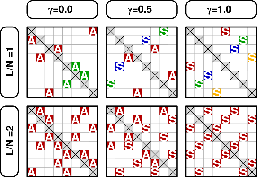
Figure 1: Examples of connectivity matrices $D$ generated by the algorithm described in Section 2.3 and in A for a reduced number of patches, $N=8$, and different combinations of $L/N$ and $\gamma$. Only non-zero entries are printed explicitly. For reasons of clarity symmetric connections are denoted by ’S’ and asymmetric connections by ’A’. The colours indicate separated closed cycles of dispersal that can be identified in the matrices. While the connectivity matrices with $L/N=1$ (upper row) are degenerate into $2$ ($\gamma=0.0$), $3$ ($\gamma=0.5$), and $4$ ($\gamma=1.0$) clusters respectively, the clusters of all three matrices generated with $L/N=2$ (lower row) already extend to the entire metapopulation. In spite of the fact that the matrices displayed here are only examples of randomly generated matrices, this trend is representative. For instance all simulations performed for $N=100$ and $L/N>2$ resulted in dispersal matrices with a single cluster only. Note that our results are based on much larger metapopulations consisting of $N=100$ patches.

Previous works demonstrated that changes in the symmetry of dispersal patterns in particular affect the local symmetry of migrant flow, since asymmetry can result in donor- and recipient-dominated patches not present in symmetric networks (Vuilleumier and Possingham, 2006). In order to isolate the effect of the degree of symmetry from these secondary effects, we focus on a specific set of dispersal patterns: we restrict our main analysis to dispersal patterns with the number of dispersal connections, $L$, being an integer multiple of $N$ randomly distributed on the patches under the constraint, that each patch obtains exactly $L/N$ in- and outgoing connections with defined degree of symmetry. The random patterns considered, hence, are regular with the connections evenly distributed to all patches available (Artzy-Randrup and Stone, 2010; Brandes and Erlebach, 2005). An algorithm efficiently generating regular random dispersal patterns for small and intermediate $L/N$ and arbitrary degrees of symmetry ($\gamma$) is detailed in A. Examples of random connectivity matrices generated for $N=8$ and different combinations of $L/N$ and $\gamma$ are exhibited in Fig. 1. Please regard that for the simulations metapopulations consisting of $N=100$ are used resulting in connectivity matrices of dimension $100\times 100$ instead.

The regular dispersal patterns we use here restrict our analysis to metapopulations with all patches connected at a fixed density independent of the choice of $\gamma$. For $L/N>2$ the largest cluster extends to the entire metapopulation independent from the degree of dispersal symmetry resulting in irreducible connectivity matrices (Caswell, 2001; Bode et al., 2006). For a detailed discussion of the impact of regularity on our results we refer to Section 4.2.

The viability of metapopulations exposed to these dispersal patterns was tested in the following manner: a sample of $100$ dispersal patterns connecting the $N=100$ patches was generated for each combination of $L/N=1,\ldots,10$ and $10$ different values of $\gamma$. For any of these patterns the viability of $10$ independent realisations of metapopulations was tested for different values of the colonisation probability $c$ according to the procedure outlined in Section 2.1, resulting in a statistics for a total of $1,000$ simulations on $100$ randomly generated connectivity matrices for every choice of $L/N$, $\gamma$, and $c$. For our main analysis we record the number of viable metapopulations out of the $1,000$ simulations and prepare the results for graphical analysis. The sensitivity of this test procedure and its interpretation with respect to the statistics of extinction times is discussed in Section 4.1.

3 Results

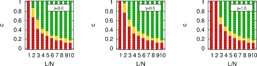
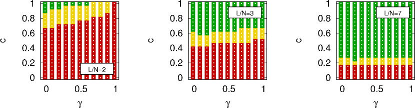
Figure 2: Results on the viability of metapopulations exposed to dispersal patterns with regular dispersal randomly generated by the algorithm described in Section 2.3 and A. In the upper row the viability is plotted as a function of the effective number of connections per patch, $L/N$, and the colonisation probability $c$. At every combination of $L/N$ and $c$ the viability of $1,000$ different dispersal patterns has been investigated. Green and red squares indicate parameters, where either all $1,000$ patterns either were viable or not. The intermediate region where some of the patterns were viable and others were not is coloured yellow. The three panels present the results for different degrees of symmetry, increasing from $\gamma=0$ (anti-symmetric dispersal patterns) on the left to $\gamma=1$ (symmetric patterns) on the right hand side. In the lower row the simulation results are presented accordingly as a function of the symmetry $\gamma$ and the colonisation probability $c$ for three different number of connections per patch, $L/N=2,3$ and $5$. Only a vanishing impact of symmetry is observed for $L/N>3$.

For each scenario $(L/N,\gamma,c)$ a total of $1,000$ simulations were performed. For straightforward statistical evaluation of the viability of metapopulations exposed to the respective conditions the simulation results were divided into three different groups, which are colour coded in the graphical presentation of the results: if all $1,000$ simulated metapopulations either went extinct or were viable the scenario is coloured red or green, respectively. Otherwise, i.e. if the number of extinct simulations out of $1,000$ is greater than $0$ but smaller than $1,000$, the scenario was coloured yellow.

The results are illustrated in Fig. 2. The three panels in the upper row show the viability of the metapopulation as a function of the number of dispersal connections per patch, $L/N$, and the colonisation probability $c$ for different values of $\gamma$: anti-symmetric dispersal ($\gamma=0.0$), asymmetric dispersal with intermediate degree of symmetry ($\gamma=0.5$), and symmetric dispersal ($\gamma=1.0$). The lower panels of Fig. 2 contain the same results, but now analysed with respect to the effect of the degree of symmetry, $\gamma$, for three different values of $L/N$. In fact, for $L/N>3$ no statistically significant impact of symmetry is observed.

4 Discussion

4.1 Interpretation and significance of results

First of all the results depicted in Fig. 2 suggest that the impact of the degree of symmetry on metapopulation viability decreases with increasing $L/N$. Already at $L/N>3$ no statistical significant impact of the degree of symmetry, i.e. no systematic differences depending on the degree of symmetry, can be detected on the basis of the scenarios and the statistical evaluation chosen.

At a small number of dispersal connections per patch ($L/N=1,2$) metapopulation viability is significantly reduced for more symmetric dispersal (Fig. 2, lower panels). The reason for this effect straightforwardly can be understood from considerations concerning the structure of the underlying dispersal patterns: Let us first focus on patterns with $L/N=1$. In this case a metapopulation with a symmetric dispersal pattern necessarily consists of a number of patches only pairwisely connected through dispersal (Figure 1). The largest closed dispersal cycle (synonymous to the giant component of the dispersal network (Berchenko et al., 2009)), hence, involves only two patches. For the particular metapopulation model applied a lower bound for the extinction probability of a pair of patches per time step is $e^{2}$. On the contrary the mean size of the largest closed dispersal cycle estimated from the $100$ dispersal patterns generated for the same conditions but antisymmetric dispersal ($\gamma=0$) was $62.7$. For $L/N=2$ the mean size of the largest cycles was $77.5$ for the symmetric dispersal matrices generated, whereas for the asymmetric case all dispersal matrices already extended to the entire metapopulation (i.e. their mean size was $100$). Hence we are faced with a percolation problem on random graphs (Callaway et al., 2000), where the percolation threshold depends on the symmetry properties of the dispersal pattern. Analysis of the eigenvalues of associated state transition matrices reveals, that the mean time to extinction of a set of patches participating in a closed cycle of dispersal increases with the size of the cycle. For this reason differences in viability at small $L/N$ are attributed to hierarchical differences of the generated matrices at only a few number of connections, namely $L/N\leq 3$. This density is much smaller then relevant cases discussed e.g. in (Vuilleumier and Possingham, 2006) as will be discussed in more detail in Section 4.3.

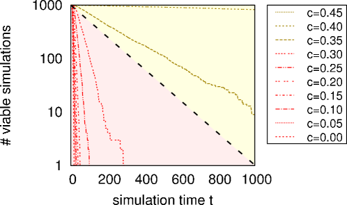
Figure 3: Extinction statistics for the metapopulations with different values of the colonisation probability $c$ connected through dispersal matrices with $\gamma=0.5$ and $L/N=4$. The individual lines indicate the number of non-extinct simulations (out of $1,000$) as a function of the simulation time. The dashed line corresponds to the upper bound for the expectation value of the number of extinct simulation for cases where all simulations went extinct, $1,000\exp(-6.9\times 10^{-3}t)$, as derived in the manuscript text. From the figure it becomes evident, that the number of non-extinct simulations after an initial relaxation phase indeed decreases exponentially in time (i.e. linear in this logarithmic plot). The upper bound approaches $1/M$ with $t\to T$, which is a general result for sufficiently large $M$ and $T$ as a Taylor expansion of expression (7) shows. For this reason the boundary line indeed exhibits the border between the cases marked red and yellow in Figure 2.

How meaningful is the statistical evaluation of the results with respect to the effect of the symmetry of dispersal patterns on expected extinction times of metapopulations? In order to approach this question we aim to derive lower and upper bounds for extinction times in the red and green regions of the figures, which then help to evaluate the graphical presentation of the results in more detail. If we disregard the initial time period of relaxation of the metapopulation to a quasistationary state, we can assume that the statistics of extinction times is exponentially distributed. This exponential distribution complies with a constant risk of metapopulation extinction per time step, which we call $r$. The chance, that a metapopulation has not gone extinct after $T$ time steps then is $(1-r)^{T}$. For every combination of parameters we perform $M$ simulations with $M=1,000$ in our case. It is then straightforward to calculate the probability $P(M|r)$ that all $M$ simulations are viable,

$$P(M|r)=(1-r)^{MT}\quad.$$ (3)

Accordingly the chance that a simulation goes extinct during the $T$ simulation steps is $1-(1-r)^{T}$, resulting in the probability $P(0|r)$ of observing $0$ viable simulations of

$$P(0|r)=\left(1-(1-r)^{T}\right)^{M}\quad.$$ (4)

More interesting, however, would be the expressions $P(r|M)$ and $P(r|0)$, the probability distributions of the metapopulation extinction risk $r$ given the fact that either all or none of the simulations are viable. These expressions straightforwardly can be calculated using Bayes’ theorem. Using uniform prior distributions we obtain

$$P(r|M) = \left(\int_{0}^{1}dr^{\prime}(1-r^{\prime})^{MT}\right)^{-1}(1-r)^{MT}\quad\mbox{and}$$ (5)

$$P(r|0) = \left[\int_{0}^{1}dr^{\prime}\left(1-(1-r^{\prime})^{T}\right)^{M}\right]^{-1}\left(1-(1-r)^{T}\right)^{M}\quad.$$ (6)

Using a maximum likelihood approach confidence intervals for $r$ can be calculated. Applying a confidence level of $95\%$ the upper bound for $r$ in cases where all simulations are viable is $5.1\times 10^{-8}$. As a lower bound for $r$ for cases where all simulations went extinct we obtain $0.057$. Since the latter result strongly depends on the prior distribution we instead use the inflection point of the sigmoid function (6) at

$$1-\left[(T-1)/(MT-1)\right]^{1/T}$$ (7)

as a more conservative estimate, which for the case of our simulations is located at approximately $6.9\times 10^{-3}$. The inverse of $r$ corresponds to the mean time to extinction. From our considerations we, hence, expect the mean time to extinction for the scenarios marked by red squares in Figure 2 to be below $6.9^{-1}\times 10^{3}\approx 145$ and the respective value for the conditions marked green to be in the order of $2\times 10^{7}$ or larger. Intermediate values are expected for the conditions marked yellow in the individual plots. Figure 3 demonstrates, that assumptions we needed to make seem to hold and that the estimates indeed reflect the underlying extinction statistics to a great extent.

Obviously the classification of the conditions by the three scenarios to a meaningful extent reflects the extinction risks of the metapopulation in a sense, that Figure 2 succeeds to highlight the main results. From the bounds for the mean extinction times to extinction derived above for the respective classes we can conclude that metapopulations in the red regions almost surely go extinct within a short time, whereas metapopulations in the green regions are likely to be persistent. The yellow region decreases in range with increasing $L/N$. That is, the transition between threatened and persistent metapopulation sharpens with increasing $L/N$.

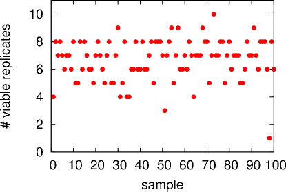
Figure 4: Extreme example of the variation in the number of viable replicates between the different samples (here: $\gamma=0.3$, $L/N=10$, $c=0.15$). In particular sample $98$ deviates strongly from the general mean. Since we can assume that the main source of variations is the stochastic simulation procedure rather than qualitative differences between the random dispersal patterns relevant for the present study, we do not investigate the within-sample variations further within the scope of this work.

The $10$ replicate simulations performed for each parameter set and each dispersal pattern in addition allow to investigate and to discuss the variability within the sample of $100$ dispersal patterns. In the regions marked red and green by definition all samples show the same behaviour. Detailed analysis of the yellow regions shows only very few cases of large variability of the number of extinct replicates between the samples. One example of rather high variability is depicted in Figure 4. Overall the differences between the random dispersal patterns generated for each scenario do not seem to be relevant for the present study, which is probably due to the decision of using regular dispersal patterns.

4.2 Impact of regularity on the results

So far we focused on regular dispersal patterns. This approach made it possible to investigate the impact of the degree of symmetry of connectivity matrices on metapopulation viability independently from other possibly confounding effects, which is important in order to assess the role of dispersal symmetry for metapopulations. Our results on regular dispersal patterns show a remarkably low effect of symmetry ($\gamma$) on the viability of metapopulations at intermediate and high density of dispersal paths, $L/N$. At low $L/N$ symmetric dispersal even results in a slightly negative effects on the viability. How do these results relate to the more general case where the dispersal network is not regular?

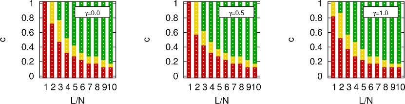
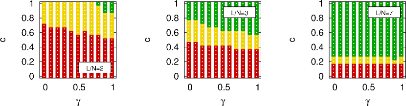
Figure 5: Results on the viability of metapopulations exposed to general dispersal patterns randomly generated by modification of the algorithm described in A. The analysis and graphical presentation of the simulation results is accordant to the procedure described in the caption of Figure 2. Please note that $L/N$ now specifies the mean number of connections per patch, while the actual number of dispersal links now can vary between patches.

In order to follow up this question we repeated the simulations accordingly, but now without the constraint of having regular dispersal networks. Technically this was implemented by skipping steps 4c and 4d of the pattern generation algorithm detailed in A, which then controls for the desired degree of symmetry only. The parameter $L/N$ now should be understood in a statistical sense, such that $L$ dispersal connections randomly were distributed between the $N$ patches resulting in a mean density of $L/N$ connections per patch. The results are depicted in Figure 5. Interestingly, the minor effect of symmetry at low density of dispersal connections now shifts to a slight advantage for metapopulations with a symmetric dispersal pattern. From $L/N\geq 7$ no significant differences with respect to the simulation results based on regular dispersal patterns (Figure 2) are observed.

In non-regular dispersal patterns the existence of isolated patches not participating in dispersal has an impact on the effective density of dispersal connections in the metapopulations (see also Bode et al., 2008). Moreover, in the case of asymmetric dispersal there exist patches that either only receive or only provide migrants, i.e. sinks or sources, and that cannot actively take part in the metapopulation dynamics (Artzy-Randrup and Stone, 2010). Since both of these effects are most distinct at small densities of the random dispersal networks, we assume that these differences basically drive the minor differences at low $L/N$ between our results on regular and the general case of random dispersal. Arguments for not assigning this effects to asymmetry in dispersal but to examine them separately are made in Section 5.

4.3 Relation to previous works

In general our results suggest essentially no direct negative effect of asymmetric dispersal on metapopulation viability at intermediate and high densities of the dispersal network, at least as far as the stochastic patch occupancy model applied in this work is concerned. This is in contrast to the findings in (Vuilleumier and Possingham, 2006) where it was concluded that extinction risk significantly increased when dispersal became asymmetric. The analysis in (Vuilleumier and Possingham, 2006) is not restricted to cases with regular dispersal only, although the relaxation of regular dispersal is not not sufficient to explain the qualitative differences in the results as shown in the previous section.

The description of the random patterns investigated in (Vuilleumier and Possingham, 2006) does not provide all information necessary for an in-depth comparison with our results. In (Vuilleumier and Possingham, 2006) the number of dispersal connections was chosen randomly for each of the $2,000$ metapopulations. Additional information provided on two particular patterns suggest that the densities are comparable or higher than the densities we investigated in our study. From our results we therefore do not expect a significant impact of dispersal asymmetry at these density of connections.

The analysis of the results in (Vuilleumier and Possingham, 2006) is based on the number of connected patches in contrast to our analysis using the global mean number of connections $L/N$. The statistics of the number of connected patches seems to differ significantly between the asymmetric and the symmetric connectivity matrices investigated, a phenomenon we were not able to reproduce. In particular the example of a symmetric random pattern with more than $85$ connections per patch but only $96$ connected patches raises questions, since the largest cycle of closed dispersal in non-regular connectivity matrices we generated always extended to at least $99$ patches for densities above $7$ connections per patch with a strong trend towards $100$ patches with increasing density. For this reason we assume, that the effects described in (Vuilleumier and Possingham, 2006) originate from differences in network topology between the investigated connectivity matrices rather than differences in dispersal asymmetry.

Bode et al. (2008) investigated the same metapopulation model as in the present work in a slightly different setup ($N=10$, $e=0.4$, and $L/N=2.6$). Instead of simulating individual realisations, the probability of metapopulations to go extinct within $100$ time steps was calculated numerically for different dispersal patterns. This method restricts the analysis to rather small metapopulations of $10$ patches. Extinction probabilities were calculated for metapopulations connected through different dispersal patterns generated by the small world algorithm (see e.g. Watts and Strogatz, 1998; Kininmonth et al., 2009) initiated with a particular symmetric dispersal pattern (Bode, pers. communication). Bode et al. (2008) concluded from qualitative graphical analysis of their simulation results, that asymmetry reduces persistence and exhibits a distinct threat to metapopulations.

The discussion of our results in Section 4.1 relates our graphical analysis to the extinction probability in a certain number of time steps, which allows for a comparison of the results. From additional simulation data we received from Bode it seems, that the negative effect in their approach is larger than what we would expect from our simulation for the general, non-regular case (Section 4.2). Additional simulations performed for metapopulations likewise subjected to non-regular dispersal patterns but reduced to the size of $10$ patches indicated a general increase in the probability of extinction but no significant impact of metapopulation size on the impact of symmetry. We therefore assume, that the differences related to symmetry observed by Bode et al. partly are owed to the fact, that the patterns in their study were generated from a particular symmetric starting configuration of the small world algorithm and that the similarity of patterns to this starting configuration correlates with the symmetry properties.

Recently another work was devoted to the effect of asymmetry on metapopulation viability (Vuilleumier et al., 2010). This work aims to cover different aspects of asymmetry simultaneously, which makes it difficult to ascribe the variety of effects observed to certain properties of dispersal matrices. One configuration, however, seems to be equivalent to the simulations we performed for general dispersal matrices in Section 4.2 for anti-symmetric and symmetric dispersal, respectively (Vuilleumier et al., 2010, p. 229, Fig. 2, right column). The results the authors obtain on these patterns are in agreement with our observations, that the degree of symmetry of dispersal matrices has no significant impact on metapopulation viability at intermediate density of dispersal connections (cp. Vuilleumier et al., 2010, p. 213, Fig. 6, difference between the plots in the right column).

5 Conclusions

We investigated the consequences of the symmetry of dispersal patterns on the viability of metapopulations. Our analyses are based on simulations of a stochastic patch occupancy model.

First we define the degree of dispersal symmetry, $\gamma$, which is based on the symmetry of the connectivity matrix (Equation 2). In order to be able to minimise possibly confounding effects we restrict our main analysis to regular dispersal patterns, where asymmetry does neither affect the homogeneity of dispersal nor the local balances of incoming and outgoing dispersal connections. For these patterns we do not see any negative effect of dispersal asymmetry. For the more general case of non-regular dispersal patterns minor negative effects of asymmetric dispersal on metapopulation viability are confirmed, but only at rather weak densities of dispersal (cp. Section 4.2). At these densities differences in dispersal symmetry generally are accompanied by other hierarchical differences of the dispersal network. This e.g. becomes evident from a neat example of a two patch metapopulation investigated in detail in (Bode et al., 2008, p. 208, Appendix A), where dispersal asymmetry by return results in a source-sink problem.

From first instance it is not self-evident whether these accompanying effects are the origin or a consequence of asymmetric dispersal, since their characteristic strongly depends on how the system of study was constructed and chosen. For realistic dispersal patterns the solution proposed in (Vuilleumier et al., 2010), namely to investigate dispersal asymmetry independent from the discussion of sources and sinks, however does not seem to work out, since these effects in general are strongly connected to one another. These correlations in the past made the investigation of asymmetric dispersal highly dependent on the system of study, which was the main difficulty in understanding the role of dispersal asymmetry. In order to resolve this problem we suggest to discuss the symmetry of dispersal patterns at large scales e.g. based on a definition similar to Equation (2) and the statistics of sources and sinks, the homogeneity of the dispersal network, and other features characterising the local flow of migrants jointly instead of in isolation.

It was the aim of the present work, to clarify the role of asymmetric dispersal and its impact on metapopulation viability. In contrast to previous studies (Vuilleumier et al., 2010; Vuilleumier and Possingham, 2006; Bode et al., 2008) we see only weak effects of asymmetric connectivity on metapopulation extinction, which suggests that natural populations with asymmetric dispersal may not per se suffer from increased extinction risks. Instead effects observed in simulations, real world data, or in the evaluation of management strategies (see e.g. Haight and Travis, 2008) might be reflected more significantly by other features of complex dispersal patterns. A promising path towards a discussion of potentially important features is taken in the investigations of the viability of metapopulations connected through a variety of different dispersal patterns as provided in (Bode et al., 2008; Artzy-Randrup and Stone, 2010). We expect that eventually only a theoretical analysis of the stochastic metapopulation model applied can reveal the features relevant for metapopulation viability.

6 Acknowledgements

We kindly acknowledge comments by Bernt Wennberg on an early version of the manuscript and suggestions by Kerstin Johannesson on a more recent version. We kindly appreciate that Michael Bode contributed simulation results and shared details on his 2008 work, (Bode et al., 2008). Furthermore we are deeply indebted to kind and constructive comments of two anonymous reviewers. This work was supported by a Linnaeus-grant from the Swedish Research Councils, VR and Formas (http://www.cemeb.science.gu.se), by FORMAS through contract 209/2008-1115 (PRJ), and by the Swedish Research Council through contract 275 621-2008-5456 (PRJ).

Appendix A Algorithm for the generation of regular dispersal patterns

Since we intended to compare cases primarily differing in their symmetry properties, we focused on regular dispersal patterns with fixed number of in- and out-going dispersal routes for every patch. For the connectivity matrices $D$ this is equivalent to the constraint that the sums over every column and every row are equal, that is

$$\sum_{k}d_{ik}=\sum_{k}d_{kj}=L/N$$ (8)

for any $i$ and $j$. Here $L$ is the total number of activated dispersal routes.

Random matrices at arbitrary degree of symmetry that are complying with Equation (8) are generated by the following algorithm, that is repeated until a matrix $D$ with $L$ non-zero elements is obtained:

1. Set $D=0$, generate a random matrix $B\in\left[0,1\right]^{N\times N}$, where $b_{ij}$ are random numbers drawn independently from an arbitrary distribution. For instance uniformly distributed random variables are suitable here. Ensure that all elements of $B$ are unique.

2. Set diagonal elements $b_{ii}$ to $10$ for all $i$.

3. Calculate the desired number of symmetric connections, $n_{s}=\gamma L$

4. Repeat until smallest element of $B$ is larger than $1$ or $\sum_{i,j}d_{ij}=L$:

   1. Identify row $i$ and column $j$ of the smallest value of $B$

   2. Set $d_{ij}=1$ and $b_{ij}=10$ (*)

   3. If $\sum_{k}d_{ik}=L/N$ set $b_{ik}=10$ for every $k$ (*)

   4. If $\sum_{k}d_{kj}=L/N$ set $b_{kj}=10$ for every $k$ (*)

   5. Switch $i$ and $j$

   6. if $n_{s}>0$ (generate symmetric connection):

      • repeat the steps marked by (*)

      • reduce $n_{s}$ by $2$

      else: (generate asymmetric connection)

      • set $b_{ij}=10$

5. Reject result if $\sum_{i,j}d_{ij}<L$.

Note that the value $10$, of course, is arbitrary. Any number greater than $1$ is suitable to ensure that the corresponding elements of $D$ are not selected by the algorithm. This algorithm randomly orders the elements of $D$ and activates them step by step. It generates random connectivity matrices with given degree of symmetry and it is sufficiently efficient for small and intermediate $L$.

The implementation of the algorithm in FORTRAN90 is straightforward (compilation tested with the GNU Fortran compiler gfortran v4.3.3):

REGULAR.F90

⬇

1PROGRAM REGULAR_CONNECTIVITY

!======================================================================

! PROGRAM REGULAR_CONNECTIVITY

! GENERATION OF REGULAR RANDOM DISPERSAL PATTERNS

! TESTED WITH GFORTRAN 4.3.3

6 ! (C) 2010 BY DAVID KLEINHANS, UNIVERSITY OF GOTHENBURG, SWEDEN

! DISTRIBUTED UNDER THE CREATIVE COMMONS ATTRIBUTION 3.0 LICENSE

!======================================================================

IMPLICIT NONE

11

INTEGER,PARAMETER::N=100 !METAPOPULATION SIZE

INTEGER,PARAMETER::MAX_REJECTIONS=1000!MAXIMUM NO OF REJECTED MATRICES

DOUBLE PRECISION::GAMMA !DEGREE OF SYMMETRY

16 INTEGER::LBYN !NO. OF CONNECTIONS PER PATCH

INTEGER::D(N,N) !CONNECTIVITY MATRIX

DOUBLE PRECISION::RAND(N,N) !RANDOM MATRIX USED FOR ORDERING OF LINKS

21 DOUBLE PRECISION::REMAINING_SYM !NO OF REMAINING SYMMETRIC CONNECTIONS

INTEGER::REJECTIONS !COUNT NUMBER OF REJECTED DISPERSAL PATTERNS

INTEGER::LOC(2) !LOCATION OF THE SMALLEST ELEMENT OF RAND

INTEGER::I,J !AUXILIARY VARIABLES, USED FOR LOOPS ONLY

LOGICAL::GRIDOK !CHECK IF GRID COMPLIES WITH CONSTRAINTS

26

! === INITIALIZE RANDOM NUMBER GENERATOR ===

CALL RANDOM_SEED

31 ! === REQUEST PARAMETERS ===

WRITE(*,”(A,I4)”)”REGULAR DISPERSAL MATRIX FOR METAPOPULATION OF SIZE N=”,N

WRITE(*,”(A)”)”PLEASE ENTER PARAMETERS:”

WRITE(*,”(A)”)”DEGREE OF SYMMETRY, GAMMA (DOUBLE PRECISION, >=0 AND <=1)?”

READ(*,*)GAMMA

36 WRITE(*,”(F8.5)”)GAMMA

WRITE(*,”(A,I4,A)”)”NO OF CONNECTIONS PER PATCH, LBYN (INTEGER, >0 AND <”,&

&(N-1)/2,”)?”

READ(*,*)LBYN

WRITE(*,”(I4)”)

41

! === GENERATE DISPERSAL PATTERN ===

GRIDOK=.FALSE.

REJECTIONS=0

DO WHILE(.NOT.GRIDOK)

46

! == STARTING CONFIGURATION: ==

! ALL LINKS INACTIVE

D=0

! CALCULATE NUMBER OF SYMMETRIC LINKS TO BE GENERATED

51 REMAINING_SYM=NINT(GAMMA*LBYN*N)

! GENERATE RANDOM NUMBER MATRIX FOR ORDERING OF LINKS

! (EXCLUDE DIAGONAL ELEMENTS BY ASSIGNING VALUE OF 10)

DO I=1,N

DO J=1,N

56 IF(I.NE.J)THEN

CALL RANDOM_NUMBER(RAND(I,J))

ELSE

RAND(I,J)=10.D0

ENDIF

61 ENDDO

ENDDO

! == ADD CONNECTIONS UNTIL NO LINKS ARE AVAILABLE ANY MORE ==

DO WHILE((MINVAL(RAND).LT.1).AND.(COUNT(D.EQ.1).LT.LBYN*N))

66

!LOCATE THE SMALLEST ELEMENT OF RAND

LOC=MINLOC(RAND)

!SET RANDOM NUMBER OF THE ELEMENT TO 10 AND ACTIVATE CORRESPONDING LINK

71 RAND(LOC(1),LOC(2))=10.D0

D(LOC(1),LOC(2))=1

!CHECK WHETHER NUMBER OF DESIRED INCOMING OR OUTGOING LINKS ALREADY

!HAS BEEN REACHED FOR THE PATCH OF FOCUS, PREVENT FURTHER LINKS IF SO

IF(COUNT(D(LOC(1),:).EQ.1).GE.LBYN)RAND(LOC(1),:)=10.D0

76 IF(COUNT(D(:,LOC(2)).EQ.1).GE.LBYN)RAND(:,LOC(2))=10.D0

!IF SYMMETRIC CONNECTIONS ARE REMAINING: MAKE THE CURRENT A SYMMETRIC ONE,

!ELSE ENSURE THAT THE REVERSE DIRECTION IS NOT ACTIVATED

IF(REMAINING_SYM.GT.0)THEN

81 D(LOC(2),LOC(1))=1

RAND(LOC(2),LOC(1))=10.D0

IF(COUNT(D(LOC(2),:).EQ.1).GE.LBYN)RAND(LOC(2),:)=10.D0

IF(COUNT(D(:,LOC(1)).EQ.1).GE.LBYN)RAND(:,LOC(1))=10.D0

REMAINING_SYM=REMAINING_SYM-2

86 ELSE

RAND(LOC(2),LOC(1))=10.

ENDIF

ENDDO

91 !CHECK WHETHER THE DESIRED NO OF LINKS HAS BEEN GENERATED

!REJECT AND RESTART IF NOT, ACCEPT THE PATTERN OTHERWISE

IF (COUNT(D.EQ.1).EQ.LBYN*N)THEN

GRIDOK=.TRUE.

ELSE

96 REJECTIONS=REJECTIONS+1

IF(REJECTIONS.LT.MAX_REJECTIONS)THEN

WRITE(*,”(A,I4,A)”)”PATTERN ”,REJECTIONS,&

&” REJECTED, RESTARTING GRID GENERATION …”

ELSE

101 WRITE(*,”(A)”)”GRID GENERATION NOT SUCCESSFULL.”

WRITE(*,”(A)”)”PLEASE TRY LOWER LBYN OR INCREASE MAX_REJECTIONS.”

STOP

ENDIF

ENDIF

106 ENDDO

! === WRITE D TO STANDARD OUTPUT ===

WRITE(*,*)”CONNECTIVITY MATRIX D:”

DO I=1,N

111 WRITE(*,”(999I1.1)”)D(I,:)

ENDDO

WRITE(*,”(A)”)”DONE!”

END PROGRAM REGULAR_CONNECTIVITY

References

- Armsworth (2002) Armsworth, P. R., 2002. Recruitment limitation, population regulation, and larval connectivity in reef fish metapopulations. Ecology 83 (4), 1092–1104.
- Artzy-Randrup and Stone (2010) Artzy-Randrup, Y., Stone, L., 08 2010. Connectivity, cycles, and persistence thresholds in metapopulation networks. PLoS Comput Biol 6 (8), e1000876.
- Barabási and Oltvai (2004) Barabási, A., Oltvai, Z., 2004. Network biology: understanding the cell’s functional organization. Nature Reviews Genetics 5 (2), 101–113.
- Berchenko et al. (2009) Berchenko, Y., Artzy-Randrup, Y., Teicher, M., Stone, L., 2009. Emergence and size of the giant component in clustered random graphs with a given degree distribution. Physical Review Letters 102 (13), 138701.
- Bode et al. (2006) Bode, M., Bode, L., Armsworth, P., 2006. Larval dispersal reveals regional sources and sinks in the Great Barrier Reef. Marine Ecology Progress Series 308, 17–25.
- Bode et al. (2008) Bode, M., Burrage, K., Possingham, H., 2008. Using complex network metrics to predict the persistence of metapopulations with asymmetric connectivity patterns. Ecological Modelling 214 (2-4), 201–209.
- Brandes and Erlebach (2005) Brandes, U., Erlebach, T. (Eds.), 2005. Network Analysis. Vol. 3418 of Lecture Notes in Computer Science. Springer Berlin.
- Callaway et al. (2000) Callaway, D., Newman, M., Strogatz, S., Watts, D., 2000. Network robustness and fragility: Percolation on random graphs. Physical Review Letters 85 (25), 5468–5471.
- Caswell (2001) Caswell, H., 2001. Matrix population models: Construction, analysis, and interpretation. Second edition. Sunderland, Massachusetts, USA: Sinauer Associates.
- Crooks and Sanjayan (2006) Crooks, K., Sanjayan, M., 2006. Connectivity conservation. Cambridge Univ Pr.
- Davis et al. (2008) Davis, S., Trapman, P., Leirs, H., Begon, M., Heesterbeek, J., 2008. The abundance threshold for plague as a critical percolation phenomenon. Nature 454 (7204), 634–637.
- Gyllenberg and Hanski (1992) Gyllenberg, M., Hanski, I., 1992. Single-species metapopulation dynamics: a structured model. Theoretical population biology(Print) 42 (1), 35–61.
- Haight and Travis (2008) Haight, R., Travis, L., 2008. Reserve design to maximize species persistence. Environmental Modeling and Assessment 13 (2), 243–253.
- Hanski (1994) Hanski, I., 1994. A practical model of metapopulation dynamics. Journal of Animal Ecology 63 (1), 151–162.
- Hanski (1999) Hanski, I., 1999. Metapopulation Ecology. Oxford University Press.
- Hanski (2002) Hanski, I., 2002. Metapopulations of animals in highly fragmented landscapes and population viability analysis. Population viability analysis, 86–108.
- Hanski and Gilpin (1997) Hanski, I., Gilpin, M., 1997. Metapopulation biology: ecology, genetics, and evolution. Academic Press, San Diego.
- Hanski and Gilpin (1998) Hanski, I., Gilpin, M., 1998. Metapopulation dynamics. Nature 396 (6706), 41–49.
- Joshi et al. (2001) Joshi, J., Schmid, B., Caldeira, M., Dimitrakopoulos, P., Good, J., Harris, R., Hector, A., Huss-Danell, K., Jumpponen, A., Minns, A., Mulder, C., Pereira, J., Prinz, A., Scherer-Lorenzen, M., Siamantziouras, A., Terry, A., Troumbis, A., Lawton, J., 2001. Local adaptation enhances performance of common plant species. Ecology Letters 4 (6), 536–544.
- Kawecki and Holt (2002) Kawecki, T., Holt, R., 2002. Evolutionary consequences of asymmetric dispersal rates. The American Naturalist 160 (3), 333–347.
- Kininmonth et al. (2009) Kininmonth, S., De’ath, G., Possingham, H., 2009. Graph theoretic topology of the Great but small Barrier Reef world. Theoretical Ecology.
- Levins (1969) Levins, R., 1969. Some demographic and genetic consequences of environmental heterogeneity for biological control. Bulletin of the Entomological Society of America 15 (2), 237–240.
- Malchow et al. (2008) Malchow, H., Petrovskii, S. V., Venturino, E., 2008. Spatiotemporal Patterns in Ecology and Epidemiology. Boca Raton: Chapman & Hall/CRC.
- McCallum and Dobson (2002) McCallum, H., Dobson, A., 2002. Disease, habitat fragmentation and conservation. Proceedings of the Royal Society of London, Series B: Biological Sciences 269 (1504), 2041–2049.
- Nathan et al. (2001) Nathan, R., Safriel, U., Noy-Meir, I., 2001. Field validation and sensitivity analysis of a mechanistic model for tree seed dispersal by wind. Ecology 82 (2), 374–388.
- Pulliam and Danielson (1991) Pulliam, H., Danielson, B., 1991. Sources, sinks, and habitat selection: a landscape perspective on population dynamics. The American Naturalist 137 (S1), 50.
- Roy et al. (2008) Roy, M., Harding, K., Holt, R., 2008. Generalizing Levins’ metapopulation model in explicit space: Models of intermediate complexity. Journal of Theoretical Biology 255 (1), 152–161.
- Roy et al. (2005) Roy, M., Holt, R., Barfield, M., 2005. Temporal autocorrelation can enhance the persistence and abundance of metapopulations comprised of coupled sinks. The American Naturalist 166 (2), 246–261.
- Sultan and Spencer (2002) Sultan, S., Spencer, H., 2002. Metapopulation structure favors plasticity over local adaptation. The American Naturalist 160 (2), 271–283.
- van Teeffelen et al. (2006) van Teeffelen, A., Cabeza, M., Moilanen, A., 2006. Connectivity, probabilities and persistence: comparing reserve selection strategies. Biodiversity and Conservation 15 (3), 899–919.
- Vuilleumier et al. (2010) Vuilleumier, S., Bolker, B. M., Lévêque, O., 2010. Effect of colonization asymmetries on metapopulation persistence. Theoretical Population Biology 78, 225–238.
- Vuilleumier and Possingham (2006) Vuilleumier, S., Possingham, H., 2006. Does colonization asymmetry matter in metapopulations? Proceedings of the Royal Society B 273 (1594), 1637.
- Wares et al. (2001) Wares, J., Gaines, S., Cunningham, C., 2001. A comparative study of asymmetric migration events across a marine biogeographic boundary. Evolution 55 (2), 295–306.
- Watts and Strogatz (1998) Watts, D., Strogatz, S., 1998. Collective dynamics of ’small world’ networks. Nature 393, 440–442.