Mask formulas for cograssmannian Kazhdan–Lusztig polynomials

Abstract.

We give two contructions of sets of masks on cograssmannian permutations that can be used in Deodhar’s formula for Kazhdan–Lusztig basis elements of the Iwahori–Hecke algebra. The constructions are respectively based on a formula of Lascoux–Schützenberger and its geometric interpretation by Zelevinsky. The first construction relies on a basis of the Hecke algebra constructed from principal lower order ideals in Bruhat order and a translation of this basis into sets of masks. The second construction relies on an interpretation of masks as cells of the Bott–Samelson resolution. These constructions give distinct answers to a question of Deodhar.

1. Introduction

Kazhdan–Lusztig polynomials were introduced in [k-l] as the entries of the transition matrix for expanding the Kazhdan–Lusztig canonical basis of the Hecke algebra in terms of the standard basis. Shortly afterwards these polynomials were shown to have important interpretations as Poincaré polynomials for the intersection cohomology of Schubert varieties [K-L2] and as a $q$-analog for the multiplicities of Verma modules [BeilBern, BryKash]. The first of these interpretations shows, in an entirely non-constructive fashion, that Kazhdan–Lusztig polynomials for Weyl groups have positive integer coefficients. While general closed formulas [billera-brenti, brenti] are known, they are fairly complicated and non-positive. A manifestly positive combinatorial rule for Kazhdan–Lusztig polynomials is still sought, as is a proof of their positivity beyond the case of Weyl groups.

Deodhar [d] proposed a framework to express Kazhdan–Lusztig polynomials positively in terms of combinatorial objects known as masks that are defined on reduced expressions. He gave two properties on sets of masks, called boundedness and admissibility, and showed that bounded admissible sets of masks can be appropriately counted to give Kazhdan–Lusztig polynomials. An independent explicit construction of bounded admissible sets of masks satisfying this characterization would then be a combinatorial proof of nonnegativity for Kazhdan–Lusztig polynomials. However, he was only able to provide a recursive method, dependent upon a priori knowledge of positivity, for constructing such a set.

At the end of [d], Deodhar mentions that it should be possible to reconcile his framework with formulas that had already appeared in the literature. One such formula is that of Lascoux and Schützenberger [LS11] for cograssmannian elements of the symmetric group $S_{n}$. In this paper we give two constructions of sets of masks which realize the Lascoux–Schützenberger formula.

The Lascoux–Schützenberger formula states that the Kazhdan–Lusztig polynomial $P_{u,w}(q)$ is given by $q$-counting edge-labellings of a rooted tree, where the tree depends only on $w$ and the precise set of valid edge-labellings depends on $u$. Our first construction is combinatorial and proceeds from this formula. This construction depends both on a basis of the Hecke algebra, which we denote $\{B^{\prime}_{w}\}$, constructed from principal lower order ideals in Bruhat order and on an interpretation of this basis in terms of sets of masks. The combinatorics of this construction takes place on heaps [viennot], first used in conjunction with Deodhar’s framework by Billey and Warrington [b-w]. We build a mask for each edge-labelling by cutting the tree as well as the heap associated to our permutation into segments and directly constructing a portion of the mask on each segment. The details of this construction involve not only heaps and trees but also some partition combinatorics.

Our second construction is based on a geometric interpretation of the Lascoux–Schützenberger formula due to Zelevinsky [zelevinsky]. He constructs some resolutions of singularities for Schubert varieties and shows geometrically that Kazhdan–Lusztig polynomials can be calculated from a cell decomposition (in the usual topological sense) of this resolution. These cells have a combinatorial indexing set with a nontrivial bijection to the Lascoux–Schützenberger trees. Our construction proceeds by constructing a mask from the combinatorial data indexing each cell. Behind our construction is a bijective association between masks on a reduced decomposition and cells on the Bott–Samelson resolution, a more general resolution of singularities for Schubert varieties. There is a map $\pi$ from the Bott–Samelson resolution to the Zelevinsky resolution. We call a set of masks geometric (with respect to the Zelevinsky resolution) if, for each cell of the Zelevinsky resolution, the mask set contains one cell in its pre-image (under $\pi$) of the same dimension. We give an algorithm for producing a geometric mask set.

Our constructions show that the problem of finding a set of masks that implements the Lascoux–Schützenberger formula is rather delicate, with choices which, while highly constrained, are numerous. Both of our constructions admit families of variations which produce different bounded admissible sets of masks. In addition, we give an example showing that our two constructions fail to conincide even after allowing any choice in their respective families of variations. These differences show that the set of masks that represent the terms of a particular cograssmannian Kazhdan–Lusztig basis element is far from canonical. Furthermore, our constructions are highly algorithmic in nature; only in a few limited cases does it seem possible to derive an explicit characterization of all the masks in our bounded admissible set, or even a characterization of the masks which evaluate to a particular element, for example the identity. However, as Kazhdan–Lusztig polynomials behave in mysterious and unexpected ways (as shown in [MW02] for example), such complexity and subtlety is not surprising.

Nevertheless, we believe there may be some important consequences and extensions to our work. As far as we know, our results provide the first example of a large class of elements for which Deodhar’s model does not produce a unique mask set. One can interpret this as evidence that Deodhar’s model is somehow incomplete in the sense that additional axioms beyond boundedness and admissibility should be included so as to produce mask sets that are canonical.

As part of our first construction, we introduce the $B^{\prime}$ basis of the Hecke algebra that is constructed from principal lower order ideals in Bruhat order. This basis has the property that both nonnegativity and monotonicity of the corresponding Kazhdan–Lusztig polynomials follow immediately in any case where the Kazhdan–Lusztig basis element $C_{w}^{\prime}$ can be expressed as a positive combination of the $B_{x}^{\prime}$. Although this positivity is not true in general, it does hold for the Kazhdan–Lusztig basis elements associated to cograssmannian permutations. In light of this, it would be interesting to characterize the elements $w$ such that $C_{w}^{\prime}$ expands nonnegatively into the $B^{\prime}$ basis.

The Lascoux–Schützenberger formula has been generalized to covexillary permutations by Lascoux [Lascoux95]. However, the Zelevinsky resolution has not been generalized to this case, though recent work of Li and Yong [LiYong10] suggest some geometric explanation for Lascoux’s formula. It would be natural to try to extend either of our constructions to all covexillary permutations, though the failure of the Zelevinsky resolution to properly generalize to the covexillary case suggests that our first construction or some other non-geometric set of masks may be better for this purpose. Work of Cortez [Cortez] suggests that the covexillary case may be an important base case to the problem of finding an explicit nonnegative formula for the Kazhdan–Lusztig polynomials in type $A$. In addition, the Lascoux–Schützenberger formula has been generalized to (co)minuscule elements in other types [boe], so it would be natural to generalize our work to this setting. The Zelevinsky resolution has also been generalized in that case [perrin, SanVan]. Finally, the Lascoux–Schützenberger formula has also been recently studied by Shegechi and Zinn-Justin [SZJ10], and it would be interesting to explicitly compare our constructions to the formulas found there.

In addition, it is an open question whether the map $\pi$ from the Bott–Samelson to the Zelevinsky resolution always restricts to a bijection over the cells we choose, since it might be the case that a cell in the Zelevinsky resolution has the same dimension as the cell we choose in its pre-image for more subtle reasons.

We now describe the contents of this paper in further detail. Sections 2 and 3 present background material and introduce the tools we need for our first construction. In Section 2 we introduce the $B^{\prime}$ basis of the Hecke algebra that is constructed from principal lower order ideals in Bruhat order. In Section 3, we show how to decompose the set of masks associated to a particular reduced expression into subsets that are compatible with the $B^{\prime}$ basis.

Our first construction is given in Section 4. We begin by recalling the combinatorial formula of Lascoux and Schützenberger [LS11] for Kazhdan–Lusztig polynomials associated to cograssmannian permutations as a sum of powers of $q$ over certain edge-labelled trees. The first main result of this section is Theorem 4.2, which states that each coefficient of our ideal basis $B_{x}^{\prime}$ in the expansion of the Kazhdan–Lusztig basis element $C_{w}^{\prime}$ corresponds precisely to one of Lascoux–Schützenberger’s edge labelled trees. The second main result is Theorem LABEL:t:main, which gives our first construction of a set of masks that realizes the formula of Lascoux–Schützenberger in Deodhar’s framework.

Before giving our second construction, we explain the connection between Bott–Samelson resolutions [BS58] and Deodhar’s theorem in Section LABEL:s:b-s. In particular, we describe the natural bijection between cells of the Bott–Samelson resolution and masks on $\mathsf{w}$. Although such a connection was pointed out in Deodhar’s paper [d] by the anonymous referee and is likely well-known to experts, the details of this connection have never before, as far as we can tell, appeared in print.

In Section LABEL:s:zel, we give our second construction. First we describe the resolutions of Zelevinsky [zelevinsky] and a map from Bott–Samelson resolutions to Zelevinsky resolutions. The main result in this section is Theorem LABEL:t:main2, which gives our second construction realizing the Lascoux–Schützenberger formula in Deodhar’s framework. At the end of this section, we give an example showing our two constructions do not coincide. More precisely, we show that our the construction of Section 4 can produce mask sets which are not geometric.

2. Bases for the Hecke algebra

2.1. Coxeter groups

Let $W$ be a Coxeter group with a generating set $S$ of involutions and relations of the form $(s_{i}s_{j})^{m(i,j)}=1$. The Coxeter graph for $W$ is the graph on the generating set $S$ with edges connecting $s_{i}$ and $s_{j}$ labelled $m(i,j)$ for all pairs $i,j$ with $m(i,j)>2$. Note that if $m(i,j)=3$ it is customary to leave the corresponding edge unlabelled. Also, if $m(i,j)=2$ then the relations imply that $s_{i}$ and $s_{j}$ commute.

We view the symmetric group $S_{n}$ as a Coxeter group of type $A$ with generators $S=\{s_{1},\dots,s_{n-1}\}$ and relations of the form $(s_{i}s_{i\pm 1})^{3}=1$ together with $(s_{i}s_{j})^{2}=1$ for $|i-j|\geq 2$ and $s_{i}^{2}=1$. The Coxeter graph of type $A_{n-1}$ is a path with $n-1$ vertices.

We may also refer to elements in the symmetric group by the 1-line notation $w=[w_{1}w_{2}\dots w_{n}]$ where $w$ is the bijection mapping $i$ to $w_{i}$. Then the generators $s_{i}$ are the adjacent transpositions interchanging the entries $i$ and $i+1$ in the 1-line notation.

An expression is any product of generators from $S$ and the length $\ell(w)$ is the minimum length of any expression for the element $w$. Such a minimum length expression is called reduced. Each element $w\in W$ can have several different reduced expressions representing it; for example, the reduced expressions for $[3412]$ are $\{s_{2}s_{3}s_{1}s_{2},s_{2}s_{1}s_{3}s_{2}\}$. Given $w\in W$, we represent reduced expressions for $w$ in sans serif font, say $\mathsf{w}=\mathsf{w}_{1}\mathsf{w}_{2}\cdots\mathsf{w}_{p}$ where each $\mathsf{w}_{i}\in S$. We call any expression of the form $s_{i}s_{i\pm 1}s_{i}$ a short-braid after A. Zelevinski (see [fan1]). We say that $x\leq w$ in Bruhat order if a reduced expression for $x$ appears as a subword (that is not necessarily consecutive) of some reduced expression for $w$. If $s_{i}$ appears as the last (first, respectively) factor in some reduced expression for $w$, then we say that $s_{i}$ is a right (left, respectively) descent for $w$; otherwise, $s_{i}$ is a right (left, respectively) ascent for $w$.

The following lemma gives a useful property of Bruhat order.

Lemma 2.1.

(Lifting Lemma) [b-b, Proposition 2.2.7] Suppose $x<w$, $s_{i}$ is a right descent for $w$, and $s_{i}$ is a right ascent for $x$. Then, $xs_{i}\leq w$ and $ws_{i}\geq x$.

It is a theorem of Matsumoto [matsumoto] and Tits [t] that every reduced expression for an element $w$ of a Coxeter group can be obtained from any other by applying a sequence of braid moves of the form

$${\underbrace{s_{i}s_{j}s_{i}s_{j}\cdots}_{m(i,j)}}\mapsto{\underbrace{s_{j}s_{i}s_{j}s_{i}\cdots}_{m(i,j)}}$$

where $s_{i}$ and $s_{j}$ are generators in $S$ that appear in the reduced expression for $w$, and each factor in the move has $m(i,j)$ letters.

As in [s1], we define an equivalence relation on the set of reduced expressions for a permutation by saying that two reduced expressions are in the same commutativity class if one can be obtained from the other by a sequence of commuting moves of the form $s_{i}s_{j}\mapsto s_{j}s_{i}$ where $|i-j|\geq 2$. If the reduced expressions for a permutation $w$ form a single commutativity class, then we say $w$ is fully commutative. A permutation $w$ is short-braid avoiding if none of its reduced words contain a short-braid; in $S_{n}$ fully commutative permutations are short-braid avoiding.

2.2. Heaps

If $\mathsf{w}=\mathsf{w}_{1}\cdots\mathsf{w}_{k}$ is a reduced expression, then following [s1] we define a partial ordering on the indices $\{1,\cdots,k\}$ by the transitive closure of the relation $i\prec j$ if $i>j$ and $\mathsf{w}_{i}$ does not commute with $\mathsf{w}_{j}$. We label each element $i$ of the poset by the corresponding generator $\mathsf{w}_{i}$. It follows from the definition that if $\mathsf{w}$ and $\mathsf{w}^{\prime}$ are two reduced expressions for a permutation $w$ that are in the same commutativity class, then the labelled posets of $\mathsf{w}$ and $\mathsf{w}^{\prime}$ are isomorphic. This isomorphism class of labelled posets is called the heap of $\mathsf{w}$, where $\mathsf{w}$ is a reduced expression representative for a commutativity class of $w$. In particular, if $w$ is fully commutative then it has a single commutativity class, and so there is a unique heap of $w$.

As in [b-w], we will represent a heap as a set of lattice points embedded in $\mathbb{N}^{2}$. To do this, we assign coordinates $(x,y)\in\mathbb{N}^{2}$ to each entry of the labelled Hasse diagram for the heap of $\mathsf{w}$ in such a way that:

1. An entry represented by $(x,y)$ is labelled $s_{i}$ in the heap if and only if $x=i$, and

2. If an entry represented by $(x,y)$ is greater than an entry represented by $(x^{\prime},y^{\prime})$ in the heap, then $y>y^{\prime}$.

Since the Coxeter graph of type $A$ is a path, it follows from the definition that $(x,y)$ covers $(x^{\prime},y^{\prime})$ in the heap if and only if $x=x^{\prime}\pm 1$, $y>y^{\prime}$, and there are no entries $(x^{\prime\prime},y^{\prime\prime})$ such that $x^{\prime\prime}\in\{x,x^{\prime}\}$ and $y^{\prime}<y^{\prime\prime}<y$. Hence, we can completely reconstruct the edges of the Hasse diagram and the corresponding heap poset from a lattice point representation. This representation will enable us to make arguments “by picture” that would otherwise be difficult to formulate. Although there are many coordinate assignments for any particular heap, the $x$ coordinates of each entry are fixed for all of them, and the coordinate assignments of any two entries only differ in the amount of vertical space between them.

Note that in contrast to conventions used in other work, we are drawing the heap so that the left side of the reduced expression occurs at the top of the picture and the right side occurs at the bottom.

Example 2.2.

One lattice point representation of the heap of $w=s_{2}s_{3}s_{1}s_{2}s_{4}$ is shown below, together with the labelled Hasse diagram for the unique heap poset of $w$.

To describe the local structure of heaps of fully commutative permutations, suppose that $x$ and $y$ are a pair of entries in the heap of $\mathsf{w}$ that correspond to the same generator $s_{i}$, so that they lie in the same column $i$ of the heap. Assume that $x$ and $y$ are a minimal pair in the sense that there is no other entry between them in column $i$. If $\mathsf{w}$ is short-braid avoiding, there must actually be two heap entries that lie strictly between $x$ and $y$ in the heap and do not commute with them. In type $A$, these entries must lie in distinct columns. This property is called lateral convexity and is known to characterize those permutations that are fully commutative [b-w].

In type $A$, the heap construction can be combined with another combinatorial model for permutations in which the entries from the 1-line notation are represented by strings. The points at which two strings cross can be viewed as adjacent transpositions of the 1-line notation. Hence, we may overlay strings on top of a heap diagram to recover the 1-line notation for the permutation by drawing the strings from top to bottom so that they cross at each entry in the heap where they meet and bounce at each lattice point not in the heap. Conversely, each permutation string diagram corresponds with a heap by taking all of the points where the strings cross as the entries of the heap.

For example, we can overlay strings on the two heaps of $[3214]$. Note that the labels in the picture below refer to the strings, not the generators.

For a more leisurely introduction to heaps and string diagrams, as well as generalizations to Coxeter types $B$ and $D$, see [billey-jones]. Cartier and Foata [cartier-foata] were among the first to study heaps of dimers, which were generalized to other settings by Viennot [viennot]. Stembridge has studied enumerative aspects of heaps [s1, s2] in the context of fully commutative elements. Green has also considered heaps of pieces with applications to Coxeter groups in [green1, green2, green3].

2.3. Hecke algebras

Given any Coxeter group $W$, we can form the Hecke algebra $\mathcal{H}$ over the ring $\mathbb{Z}[q^{1/2},q^{-1/2}]$ with basis $\{T_{w}:w\in W\}$ and relations:

(2.1) $$T_{s}T_{w}= T_{sw}\text{ for }\ell(sw)>\ell(w)$$

(2.2) $$T_{s}T_{w}= (q-1)T_{w}+qT_{sw}\text{ for }\ell(sw)<\ell(w)$$

where $T_{1}$ corresponds to the identity element. In particular, this implies that

$$T_{w}=T_{\mathsf{w}_{1}}T_{\mathsf{w}_{2}}\dots T_{\mathsf{w}_{p}}$$

whenever $\mathsf{w}_{1}\mathsf{w}_{2}\dots\mathsf{w}_{p}$ is a reduced expression for $w$. Also, it follows from (2.2) that the basis elements $T_{w}$ are invertible. Observe that when $q=1$, the Hecke algebra $\mathcal{H}$ becomes the group algebra of $W$.

Let $\{C_{w}^{\prime}:w\in W\}$ denote the basis of $\mathcal{H}$ defined by Kazhdan and Lusztig [k-l]. This basis is invariant under the ring involution on the Hecke algebra defined by $\overline{q^{1/2}}=q^{-1/2}$, $\overline{T_{w}}=(T_{w^{-1}})^{-1}$; we denote this involution with a bar over the element. The Kazhdan–Lusztig polynomials $P_{x,w}(q)$ describe how to change between the $T$ and $C^{\prime}$ bases of $\mathcal{H}$:

$$C_{w}^{\prime}=q^{-\frac{1}{2}\ell(w)}\sum_{x\leq w}P_{x,w}(q)T_{x}.$$

The $C_{w}^{\prime}$ are defined uniquely to be the Hecke algebra elements that are invariant under the bar involution and have expansion coefficients as above, where $P_{x,w}$ is a polynomial in $q$ required to satisfy

$$\text{degree }P_{x,w}(q)\leq\frac{\ell(w)-\ell(x)-1}{2}$$

for all $x<w$ in Bruhat order and $P_{w,w}(q)=1$ for all $w$. We use the notation $C_{w}^{\prime}$ to be consistent with the literature because there is already a related basis denoted $C_{w}$.

The following open conjecture is one of the motivations for our work. This conjecture is known to be true in a number of special cases including when the Coxeter group is finite or affine [K-L2].

Conjecture 2.3.

(Nonnegativity Conjecture) [k-l] The coefficients of $P_{x,w}(q)$ are nonnegative in the Hecke algebra associated to any Coxeter group.

In addition, there is a related conjecture that implies nonnegativity and has been proven for finite and affine Coxeter groups [irving, BM].

Conjecture 2.4.

(Monotonicity Conjecture) If $x\leq y\leq w$ in a Coxeter group $W$, then $P_{x,w}(q)-P_{y,w}(q)\in\mathbb{N}[q]$.

We now consider another basis for the Hecke algebra $\mathcal{H}$.

Proposition 2.5.

Let $w\in W$. Define

$$B_{w}^{\prime}=q^{-\frac{1}{2}\ell(w)}\sum_{x\leq w}T_{x}.$$

Then, $\{B_{w}^{\prime}:w\in W\}$ is a linear basis of $\mathcal{H}$.

Proof.

By Möbius inversion together with the fact that Bruhat order is Eulerian, proved independently by Verma [verma] and Deodhar [deodhar_mobius], we can recover the $T_{w}$ basis elements uniquely as

$$T_{w}=\sum_{x\leq w}(-1)^{\ell(w)-\ell(x)}q^{\frac{1}{2}\ell(x)}B_{x}^{\prime}.$$

Hence, $\{B_{w}^{\prime}:w\in W\}$ forms a basis of $\mathcal{H}$. ∎

Observe that when $C_{w}^{\prime}$ can be expressed as a positive polynomial combination of $B_{x}^{\prime}$, we obtain both nonnegativity and monotonicity in the sense of Conjectures 2.3 and 2.4. Although $C_{w}^{\prime}$ cannot be expressed as a positive polynomial combination of $B_{x}^{\prime}$ in general, $C_{w}^{\prime}$ can be so expressed when $w$ is cograssmannian do have this property, as we will see in Theorem 4.2.

We say $w\in W$ is rationally smooth if $P_{x,w}(q)=1$ for all $x\leq w$. This terminology arises because, when $W$ is a finite Weyl group, it follows from [K-L2] that $w$ indexes a rationally smooth Schubert variety precisely when $w$ is a rationally smooth element. Observe that when $w$ is rationally smooth, the basis element $B_{w}^{\prime}$ is exactly equal to the Kazhdan–Lusztig basis element $C_{w}^{\prime}$.

3. Deodhar’s model and masks with prescribed defects

The main object of this work is to give formulas for Kazhdan–Lusztig polynomials of cograssmannian permutations in terms of the combinatorial model introduced by Deodhar [d] and further developed by Billey–Warrington [b-w]. We now proceed to describe this model. Fix a reduced expression $\mathsf{w}=\mathsf{w}_{1}\mathsf{w}_{2}\cdots\mathsf{w}_{p}$. Define a mask $\sigma$ associated to the reduced expression $\mathsf{w}$ to be any binary vector $(\sigma_{1},\ldots,\sigma_{p})$ of length $p=\ell(w)$. Every mask corresponds to a subexpression of $\mathsf{w}$ defined by $\mathsf{w}^{\sigma}=\mathsf{w}_{1}^{\sigma_{1}}\cdots\mathsf{w}_{p}^{\sigma_{p}}$ where

$$\mathsf{w}_{j}^{\sigma_{j}}=\begin{cases}\mathsf{w}_{j}&\text{ if }\sigma_{j}=1\\ \text{1}&\text{ if }\sigma_{j}=0.\end{cases}$$

Each $\mathsf{w}^{\sigma}$ is a product of generators so it determines an element of $W$. For $1\leq j\leq p$, we also consider initial sequences of a mask denoted $\sigma[j]=(\sigma_{1},\ldots,\sigma_{j})$, and the corresponding initial subexpression $\mathsf{w}^{\sigma[j]}=\mathsf{w}_{1}^{\sigma_{1}}\cdots\mathsf{w}_{j}^{\sigma_{j}}$. In particular, we have $\mathsf{w}^{\sigma[p]}=\mathsf{w}^{\sigma}$. We also use this notation to denote initial sequences of expressions, so $\mathsf{w}[j]=\mathsf{w}_{1}\cdots\mathsf{w}_{j}$.

We say that a position $j$ (for $2\leq j\leq p$) of the fixed reduced expression $\mathsf{w}$ is a defect with respect to the mask $\sigma$ if

$$\mathsf{w}^{\sigma[j-1]}\mathsf{w}_{j}<\mathsf{w}^{\sigma[j-1]}.$$

Note that the defect status of position $j$ does not depend on the value of $\sigma_{j}$. We say that a defect position is a zero-defect if it has mask-value 0, and call it a one-defect if it has mask-value 1. We call a position that is not a defect a plain-zero if it has mask-value 0, and we call it a plain-one if it has mask-value 1.

Let $d_{\mathsf{w}}(\sigma)$ denote the number of defects of $\mathsf{w}$ for the mask $\sigma$. We will use the notation $d(\sigma)=d_{\mathsf{w}}(\sigma)$ if the reduced word $\mathsf{w}$ is fixed. Deodhar’s framework gives a combinatorial interpretation for the Kazhdan–Lusztig polynomial $P_{x,w}(q)$ as the generating function for masks $\sigma$ on a reduced expression $\mathsf{w}$ with respect to the defect statistic $d(\sigma)$. We begin by considering subsets of the set

$$\mathcal{S}=\{0,1\}^{\ell(w)}.$$

of all possible masks on $\mathsf{w}$. For $\mathcal{E}\subset\mathcal{S}$, we define a prototype for $P_{x,w}(q)$:

$$P_{x}(\mathcal{E})=\sum_{\begin{subarray}{c}\sigma\in\mathcal{E}\\ \mathsf{w}^{\sigma}=x\end{subarray}}q^{d(\sigma)}$$

and a corresponding prototype for the Kazhdan–Lusztig basis element $C_{w}^{\prime}$:

$$h(\mathcal{E})=q^{-{1\over 2}\ell(w)}\sum_{\sigma\in\mathcal{E}}q^{d(\sigma)}T_{\mathsf{w}^{\sigma}}.$$

Definition 3.1.

[d] Fix a reduced word $\mathsf{w}=\mathsf{w}_{1}\mathsf{w}_{2}\dots\mathsf{w}_{k}$. We say that $\mathcal{E}\subset\mathcal{S}$ is admissible on $\mathsf{w}$ if:

1. $\mathcal{E}$ contains $\sigma=(1,1,\dots,1)$.

2. $\mathcal{E}=\tilde{\mathcal{E}}$ where $\tilde{\sigma}=(\sigma_{1},\sigma_{2},\dots,\sigma_{k-1},1-\sigma_{k})$.

3. $h(\mathcal{E})=\overline{h(\mathcal{E})}$ is invariant under the bar involution on the Hecke algebra.

We say that $\mathcal{E}$ is bounded on $\mathsf{w}$ if $P_{x}(\mathcal{E})$ has degree $\leq{1\over 2}(\ell(w)-\ell(x)-1)$ for all $x<w$ in Bruhat order.

Theorem 3.2.

[d] Let $x,w$ be elements in any Coxeter group $W$, and fix a reduced expression $\mathsf{w}$ for $w$. If $\mathcal{E}\subset\mathcal{S}$ is bounded and admissible on $\mathsf{w}$, then

$$P_{x,w}(q)=P_{x}(\mathcal{E})=\sum_{\begin{subarray}{c}\sigma\in\mathcal{E}\\ \mathsf{w}^{\sigma}=x\end{subarray}}q^{d(\sigma)}$$

and hence

$$C_{w}^{\prime}=h(\mathcal{E})=q^{-{1\over 2}\ell(w)}\sum_{\sigma\in\mathcal{E}}q^{d(\sigma)}T_{\mathsf{w}^{\sigma}}.$$

If a mask has no defect positions at all, then we say it is a constant mask on the reduced expression $\mathsf{w}$ for the element $\mathsf{w}^{\sigma}$. This terminology arises from the fact that these masks correspond precisely to the unique constant term in the Kazhdan–Lusztig polynomial $P_{x,w}(q)$ in the combinatorial model above. Other authors [marsh-rietsch, rietsch-williams] have used the term “positive distinguished subexpression” to define an equivalent notion.

Definition 3.3.

Let $\mathsf{w}=\mathsf{w}_{1}\mathsf{w}_{2}\cdots\mathsf{w}_{p}$ be a fixed reduced expression for an element $w\in W$. Suppose $P\subset\{2,3,\ldots p\}$. Define

$$\mathcal{F}_{\mathsf{w}}^{P}=\{\text{ masks $\sigma$ on $\mathsf{w}$ with defects precisely at the positions in $P$ }\}.$$

The following result generalizes [d, Proposition 2.3(iii)] which has been used in the work [marsh-rietsch] related to totally nonnegative flag varieties, as well as [armstrong] in the context of sorting algorithms on Coxeter groups. See [jones-match] for a derivation of the Möbius function of Bruhat order based on a specialization of this result.

Lemma 3.4.

Let $\mathsf{w}$ be a reduced expression for an element $w\in W$. Then, each $x\in W$ occurs at most once in $\{\mathsf{w}^{\sigma}:\sigma\in\mathcal{F}_{\mathsf{w}}^{P}\}$. In fact, the set of elements

$$F_{\mathsf{w}}^{P}:=\{\mathsf{w}^{\sigma}:\sigma\in\mathcal{F}_{\mathsf{w}}^{P}\}$$

is a lower order ideal in the Bruhat order of $W$. In other words, if $v\in F_{\mathsf{w}}^{P}$ and $u\leq v$, then $u\in F_{\mathsf{w}}^{P}$.

Proof.

The constraint that $\sigma$ have defects precisely at the positions in $P$ forces there to be at most one mask $\sigma$ on $\mathsf{w}$ for $x$. We describe an algorithm to construct such a mask.

Let $r_{p+1}(x)=x$ and $i=p$. We inductively assign

$$\sigma_{i}:=\begin{cases}0&\text{ if ($i\notin P$ and $\mathsf{w}_{i}$ is a right ascent for $r_{i+1}(x)$) or }\\ &\text{ ($i\in P$ and $\mathsf{w}_{i}$ is a right descent for $r_{i+1}(x)$)}\\ 1&\text{ otherwise }\\ \end{cases}\ \$$

$$\text{ and }\ \ \ \ r_{i}(x):=\begin{cases}r_{i+1}(x)&\text{ if ($i\notin P$ and $\mathsf{w}_{i}$ is a right ascent for $r_{i+1}(x)$) }\\ &\text{ or ($i\in P$ and $\mathsf{w}_{i}$ is a right descent for $r_{i+1}(x)$)}\\ r_{i+1}(x)\cdot\mathsf{w}_{i}&\text{ otherwise }\\ \end{cases}$$

for each $i$ from $p$ down to $1$. An inductive argument on the length of $\mathsf{w}$ shows that the assignments given above are the only ones that can produce a mask for $x$ in $\mathcal{F}_{\mathsf{w}}^{P}$. Hence, there is at most one mask for $x$ in $\mathcal{F}_{\mathsf{w}}^{P}$. Observe that the algorithm succeeds if and only if $r_{1}(x)$ is the identity.

Suppose the algorithm succeeds in constructing a mask in $\mathcal{F}_{\mathsf{w}}^{P}$ for $y\leq w$. If $x<y$ and we run the algorithm for both elements simultaneously, we initially have $r_{p+1}(x)=x\leq y=r_{p+1}(y)$. Observe that for each $i\leq p$, if we have $r_{i+1}(x)\leq r_{i+1}(y)$, then the algorithm considers right multiplying these elements by the same $s_{i}$ and whether $i\in P$ or not is the same for both elements $r_{i+1}(x)$ and $r_{i+1}(y)$. Therefore, by the Lifting Lemma 2.1 we have $r_{i}(x)\leq r_{i}(y)$. Since $r_{1}(y)=1$, this implies by induction that $r_{1}(x)=1$ so the algorithm succeeds for all $x<y$. Hence, $F_{\mathsf{w}}^{P}$ is a lower ideal in Bruhat order. ∎

For example, if $P=\emptyset$ then $\mathcal{F}_{\mathsf{w}}^{P}$ corresponds to the set of masks on $\mathsf{w}$ with no defects at all. In this case, $F_{\mathsf{w}}^{\emptyset}$ is the Bruhat interval $[1,w]$. Since the constant term of every Kazhdan–Lusztig polynomial $P_{x,w}(q)$ is 1 when $x\leq w$, we see that the masks in $\mathcal{F}_{\mathsf{w}}^{\emptyset}$ correspond precisely to the constant terms of $P_{x,w}(q)$.

Example 3.5.

If $W=A_{4}$, $\mathsf{w}=s_{2}s_{1}s_{3}s_{2}s_{3}$, and $P=\{5\}$, then $F_{\mathsf{w}}^{P}$ has maximal elements $s_{2}s_{3}s_{2}$ and $s_{2}s_{1}s_{3}$. The mask for $s_{2}s_{1}$ is

$$s_{2}$$

1 1 1 0 1

as a result of

$$r_{6}(x)=s_{2}s_{1},r_{5}(x)=s_{2}s_{1}s_{3}=r_{4}(x),r_{3}(x)=s_{2}s_{1},r_{2}(x)=s_{2},r_{1}(x)=1.$$

4. The cograssmannian construction

4.1. The Lascoux–Schützenberger formula

We now restrict to the case where $w$ is a permutation with at most one right ascent. We call such permutations cograssmannian. Following [Brenti98, Section 6], we describe a formula for $C_{w}^{\prime}$ when $w$ is cograssmannian that is originally due to Lascoux and Schützenberger [LS11]. Lascoux [Lascoux95] has generalized this formula to the case where $w$ is covexillary; a permutation $w$ is covexillary if there do not exist indices $i_{1}<i_{2}<i_{3}<i_{4}$ for which $w(i_{3})<w(i_{4})<w(i_{1})<w(i_{2})$.

Fix a cograssmannian permutation $w$, and let $s_{z}$ be the unique right ascent of $w$. Then, let $J=S\setminus\{s_{z}\}$ and $W_{J}$ be the corresponding parabolic subgroup of $W$. By the parabolic decomposition (see [b-b, Proposition 2.4], for example), there is a unique reduced decomposition $w=vw_{0}^{J}$ where $v$ is a minimal length coset representative in $W/W_{J}$ and $w_{0}^{J}$ is the unique element of maximal length inside the parabolic subgroup $W_{J}$. Here, $v$ has a unique right descent, so we say that it is grassmannian. Also, this implies that $v$ is fully-commutative.

Since $v$ has a unique commutativity class, we can assume that the heap of $w$ has a prescribed form in which $w_{0}^{J}$ is the product of

$$(s_{1}s_{2}\cdots s_{z-1})(s_{1}s_{2}\cdots s_{z-2})\cdots\text{ and }(s_{n-1}s_{n-2}\cdots s_{z+1})(s_{n-1}s_{n-2}\cdots s_{z+2})\cdots.$$

We now fix a reduced expression $\mathsf{w}$ belonging to this commutativity class. Figure 1 illustrates a typical cograssmannian heap. Recall that in contrast to conventions used in other work, we draw the heap so that the left side of the reduced expression occurs at the top of the picture and the right side occurs at the bottom. This allows the partition associated to $v$ to appear inside the heap in the “Russian” style. Here,

$$v=s_{1}s_{5}s_{7}s_{2}s_{4}s_{6}s_{3}s_{5}s_{4}$$

$$w_{0}^{J}=s_{1}s_{2}s_{3}s_{1}s_{2}s_{1}s_{7}s_{6}s_{5}s_{7}s_{6}s_{7}$$

and $w=vw_{0}^{J}$.

Figure 1. Heap of a cograssmannian element

We consider the ridgeline of the heap of $w$ to be the lattice path formed from the maximal entry of the heap of $v$ in each column. These entries naturally form a lattice path in which the entry in column $i+1$ is either just above or just below the entry in column $i$. Record this lattice path as a string of parentheses where “(” corresponds to a down-move, and “)” corresponds to an up-move, reading left to right along the ridgeline. In the example shown in Figure 1, the parentheses would be

$$(\ (\ )\ )\ (\ ).$$

Next, we form a rooted tree $T(w)$ by matching these parentheses. Each vertex of the tree corresponds to a matching pair “( …)” of parentheses, and one vertex is a descendent of another if and only if its pair of parentheses is enclosed by the other pair. Each consecutive matching pair is called a valley, and the valleys are the leaves of the tree. In addition, we add a single additional root node that is attached to all maximal elements of the tree. The result is denoted $T(w)$.

Next, we define certain nonnegative integers called capacities that are assigned to the leaves of the tree $T(w)$. Each leaf corresponds to some valley say in column $j$ of the ridgeline, and the capacity of the valley is defined to be the number of entries in the heap of $v$ in column $j$. In other words, the capacity is the number of levels of the heap between the valley and the entries of $w_{0}^{J}$.

In the running example, $T(w)$ is

where we have indicated the capacities of the leaf nodes.

Finally, we define $A_{w}$ to be the set of edge-labelings of $T(w)$ with entries of $\mathbb{Z}_{\geq 0}$ such that:

1. Labels weakly increase along all paths from the root to any leaf, and

2. No edge that is adjacent to a leaf node has a label that strictly exceeds the capacity of the leaf.

Let $t\in A_{w}$ be an edge-labelled tree and denote the sum of the edge labels by $|t|$. We associate a permutation $x\leq w$ to $t$. Begin with the heap of $\mathsf{w}=vw_{0}^{J}$ as described above. Consider each valley column $j$. If the corresponding leaf edge is labelled by $m\in\mathbb{Z}_{\geq 0}$, then set the top $m$ entries in column $j$ to have mask-value 0, and also set all of the entries that lie above these entries in the heap to have mask-value 0. Once this has been done for each valley, we are left with a constant mask $\gamma(t)$ on $\mathsf{w}$ that encodes a cograssmannian element; we denote this element by $x(t)$, so $x(t)=\mathsf{w}^{\gamma(t)}$. Note that it is possible for some leaves to implicitly zero out other leaves above. If $t$ and $t^{\prime}$ have the same leaf edge labels, then $x(t)=x(t^{\prime})$.

Example 4.1.

The valid edge labelings of $T(w)$ are

                         

Let $t$ be the second of these edge-labelled trees. Then $x(t)$ is obtained by starting with the heap of $w$ and then “zeroing out” the entries above the valley in column $s_{6}$ in the heap. The constant mask $\gamma(t)$ that is associated to $x(t)$ is shown in Figure 2. Hence, $x(t)$ is

$$x(t)=(s_{1}s_{2}s_{4}s_{3}s_{5}s_{4})(s_{1}s_{2}s_{3})(s_{1}s_{2})(s_{1})(s_{7}s_{6}s_{5})(s_{7}s_{6})(s_{7}).$$

Figure 2. Constant mask $\gamma(t)$ for $x(t)$

We are now in a position to state our first main result that each coefficient of $B_{x}^{\prime}$ in $C_{w}^{\prime}$ corresponds precisely to one of Lascoux–Schützenberger’s edge labelled trees.

Theorem 4.2.

Let $w$ be a cograssmannian permutation. We have

$$C_{w}^{\prime}=q^{-\frac{1}{2}\ell(w)}\sum_{t\in A_{w}}q^{d_{\mathsf{w}}(t)}B_{x(t)}^{\prime}$$

where $d_{\mathsf{w}}(t)=|t|+\frac{1}{2}\ell(x(t))$.

Proof.

Let $s_{z}$ be the unique right ascent of $w$, and define $J=S\setminus\{s_{z}\}$ with the corresponding parabolic subgroup of $W$ denoted $W_{J}$. Let $x\leq w$. Then there is a unique reduced parabolic decomposition of the form $x=vu$ where $v\in W^{J}$, so $v$ is grassmannian with $s_{z}$ as the unique right descent, and $u\in W_{J}$. Let $\tilde{x}$ be $vw_{0}^{J}$ where $w_{0}^{J}$ is the unique longest element of $W_{J}$. Then $\tilde{x}$ is cograssmannian, and since we can obtain $\tilde{x}$ from $x$ using right multiplication by elements of $J=D_{R}(w)$, we have by [k-l] that $P_{x,w}(q)=P_{\tilde{x},w}(q)$.

Hence,

$$C_{w}^{\prime}=q^{-\frac{1}{2}\ell(w)}\sum_{x\leq w}P_{x,w}(q)T_{x}=q^{-\frac{1}{2}\ell(w)}\sum_{x\leq w}P_{\tilde{x},w}(q)T_{x}.$$

Lascoux and Schützenberger [LS11] showed that $P_{\tilde{x},w}(q)=\sum_{t}q^{|t|}$ when $w$ and $\tilde{x}$ are cograssmannian. (See also [Brenti98, Theorem 6.10] for another description of this theorem.) Here, the sum is over the set $A_{\tilde{x},w}$ of all edge labelled trees from $A_{w}$ having leaf capacities given by the number of mask-value 0 entries in a given valley column of the constant mask for $\tilde{x}$ on $w=vw_{0}^{J}$. Hence,

$$C_{w}^{\prime}=q^{-\frac{1}{2}\ell(w)}\sum_{x\leq w}\sum_{t\in A_{\tilde{x},w}}q^{|t|}T_{x}.$$

Next, fix a tree $t\in A_{w}$, and let $I(t)$ be the set of elements $x$ that have $t$ contributing to the coefficient of $T_{x}$ in the expansion of $C_{w}^{\prime}$. To be explicit, $I(t)$ consists of all elements $x$ such that the grassmannian part of the unique constant mask for $\tilde{x}$ has at least the number of mask-value 0 entries in a given valley column as the corresponding leaf edge label of $t$. Then, we can rewrite the equation as

$$C_{w}^{\prime}=q^{-\frac{1}{2}\ell(w)}\sum_{t\in A_{w}}\sum_{x\in I(t)}q^{|t|}T_{x}.$$

We claim that $I(t)$ is a principal lower order ideal in Bruhat order on $W$, with maximum element $x(t)$.

First, suppose $x\in I(t)$ and $y<x$. Then we have $y^{J}\leq x^{J}$ by [b-b, Proposition 2.5.1], and this implies $\tilde{y}\leq\tilde{x}$. Thus, the number of zeros in each leaf column of $\tilde{y}$ is greater than or equal to the number of zeros in each leaf column of $\tilde{x}$. Hence, the leaf capacities for the trees in $A_{\tilde{y},w}$ are greater than or equal to the leaf capacities for the trees in $A_{\tilde{x},w}$. Therefore, $y\in I(t)$, proving that $I(t)$ is a Bruhat lower order ideal.

Since $\tilde{x}\in I(t)$ whenever $x\in I(t)$, we observe that any Bruhat maximal element of $I(t)$ must be cograssmannian. Moreover, it follows from the definition of $I(t)$ that to construct a Bruhat maximal element of $I(t)$, we must precisely follow the procedure described to construct $x(t)$. The cograssmannian condition forces the mask value 0 entries while the Bruhat maximal condition forces all the other entries to have mask value 1. Hence, $x(t)$ is the unique Bruhat maximal element in $I(t)$.

Thus $\sum_{x\in I(t)}q^{|t|}T_{x}=q^{|t|+\frac{1}{2}\ell(x(t))}B_{x(t)}^{\prime}$, and the formula is proved. ∎

To conclude the running example, we have that $C_{w}^{\prime}$ is given by 6 terms

$$C_{w}^{\prime}=B_{w}^{\prime} +q^{-\frac{1}{2}}B_{s_{6}s_{7}s_{5}w}^{\prime}+q^{-\frac{3}{2}}B_{s_{3}s_{2}s_{4}s_{1}s_{5}w}^{\prime}+q^{-\frac{3}{2}}B_{s_{3}s_{2}s_{4}s_{6}s_{1}s_{5}s_{7}w}^{\prime}$$

$$+q^{-\frac{1}{2}}B_{s_{3}s_{2}s_{4}s_{1}s_{5}w}^{\prime}+q^{-\frac{1}{2}}B_{s_{3}s_{2}s_{4}s_{6}s_{1}s_{5}s_{7}w}^{\prime}$$

corresponding precisely to the 6 edge labelled trees shown in Example 4.1. Hence, the expansion of $C_{w}^{\prime}$ into $B^{\prime}$ basis elements has a combinatorial interpretation when $w$ is cograssmannian. It would be interesting to know whether there exist other classes of elements $w$ for which $C_{w}^{\prime}$ always expands nonnegatively into the $B^{\prime}$ basis.

4.2. Masks for cograssmannian permutations

Our next goal is to use the main result of Section 3 to give a set of masks on $\mathsf{w}$ that encode $C_{w}^{\prime}$. We approach this by encoding each term $q^{|t|+\frac{1}{2}\ell(x(t))}B_{x(t)}^{\prime}$ from the formula of Theorem 4.2 as $\sum_{\sigma\in\mathcal{F}_{\mathsf{w}}^{P(t)}}q^{|P(t)|}T_{\mathsf{w}^{\sigma}}$ for some set of defect positions $P(t)$. By Lemma 3.4, it suffices to give a single mask $\sigma(t)$ with $|t|$ defects that encodes the element $x(t)$, because the other elements of $B_{x(t)}^{\prime}$ can all be encoded by masks in $\mathcal{F}_{\mathsf{w}}^{P(t)}$ with defects in the same positions $P(t)$ as $\sigma(t)$. Note that there are generally several ways to construct an appropriate $\sigma(t)$, and these different constructions may produce different mask sets.

Preserving the notation of the previous section, let $T(w)$ be the unlabelled tree constructed in the Lascoux–Schützenberger algorithm. Let $t\in A_{w}$ be one of the valid edge labelings of the tree $T(w)$. Each leaf of $t$ corresponds to a valley column in the heap of $\mathsf{w}=vw_{0}^{J}$. Let $\gamma(t)$ be the unique constant mask for $x(t)$ on $\mathsf{w}$. Recall that this mask is obtained by zeroing out entries in the heap of $\mathsf{w}$ starting from valley columns as specified by the leaf labels of $t$.

Definition of valley statistics: Fix $\mathsf{w}$ and $t$. Each valley in the ridgeline of the heap of $\mathsf{w}$ has several parameters associated to it. Let $v$ be a valley column of the heap, and let $p(v)$ be the number of mask-value 0 entries in column $v$ in $\gamma(t)$. We call these mask-value 0 entries in the heap of $\gamma(t)$ valley entries. We number these sequentially so that the lowest such entry in the picture is the first valley entry, and the top valley entry is the $p(v)$-th valley entry. Define $q(v)$ to be the number of “up steps” in the ridgeline lying between $v$ and the next peak in the ridgeline to the right of $v$. We say that the $i$th valley diagonal consists of the entries extending to the southeast in the heap from the $i$th valley entry. If there exist mask-value 1 entries below the $i$th entry of the $i$th valley diagonal in $\gamma(t)$, then we say that the $i$th valley diagonal is not zeroed out. Otherwise, we say that the $i$th valley diagonal is zeroed out. These zeroed out diagonals arise from mask-value 0 entries in a valley column further to the right in the construction of $\gamma(t)$, so once a valley column is zeroed out, all higher valley columns are also zeroed out. Let $r(v)$ be the number of valley diagonals that are not zeroed out.

Definition of segments and regions: We now define the segment associated to $v$ to be the collection of entries of the heap of $\mathsf{w}$ given as the following union of regions. Region $\mathfrak{1}$ is defined to be the top $p(v)$ entries in columns $v$ through $v+q(v)$. Region $\mathfrak{2}$ is defined to be the entries of the $r(v)$ valley diagonals that are not zeroed out and do not lie in region $\mathfrak{1}$. Region $\mathfrak{3}$ is defined to be those entries of columns $v$ through $v+q(v)$ that lie on zeroed out valley diagonals and do not lie in region $\mathfrak{1}$.

For example, Figure 3 illustrates how a particular heap decomposes into segments. The mask-values in Figure 3 come from the constant mask $\gamma(t)$ that corresponds to a particular edge-labelled tree $t$ (that we have not specified completely). The labels $a,b,\ldots,k$ correspond to the edge labels from the tree $t$ as shown in Figure 4. Figure 5 shows how one of the segments in Figure 3 decomposes into regions.

Figure 3. The heap broken into segments

Figure 4. Edge-labelled trees give ridgeline labels

Figure 5. A single segment broken into regions

The following lemma, which allows us to work segment by segment in specifying the mask $\sigma(t)$, follows immediately from the definition.

Lemma 4.3.

Suppose $v$ and $v^{\prime}$ are distinct valley columns in the heap of $\mathsf{w}$. Then the entries in the segment associated to $v$ are disjoint from the entries of the segment associated to $v^{\prime}$.

Definition of $\lambda(v,t)$: Recall that the vertices of $T(w)$ correspond to pairs of edges in the ridgeline that lie at the same level in the heap such that, in the lattice path associated to the ridgeline, the left edge is a “down step”, and the right edge is an “up step”. Since we also adjoin a root vertex to the tree, we can associate each vertex, and hence each pair of matching steps in the ridgeline, to the unique edge above it in the rooted tree. Although each edge in $T(w)$ is represented by two different steps in the ridgeline, we choose the “up steps” as our representatives for a given edge in the tree $T(w)$. (Observe that this is a choice from which a dual construction could be developed.) We label these “up steps” by the edge label given in $t$. Restricting to a particular segment associated with valley $v$, let $e_{1},e_{2},\ldots,e_{q(v)}$ denote these edge labels associated with the “up steps” of the ridgeline in columns $v$ through $v+q(v)$, where the edges are ordered sequentially with $e_{1}$ labeling the leaf edge which is closest to the valley $v$. The edge labels form a partition

$$p(v)\geq e_{1}\geq e_{2}\geq\cdots\geq e_{q(v)}\geq 0$$

that we denote by $\lambda(v,t)$. Observe that $e_{1}<p(v)$ precisely when there exists a valley to the left or right of $v$ with a large leaf edge label that “zeros out” entries above in the construction of $\gamma(t)$.

For example, in Figure 3 the labels $d,e,\ldots,j$ give the parts of the the partition $\lambda(v,t)$ where $v$ is the fourth valley column from the left and $t$ is the tree shown in Figure 4.

Definition of the mask $\sigma(t)$: We are now in a position to define our mask $\sigma(t)$ for $x(t)$ on $\mathsf{w}$, working segment by segment. Fix a valley column $v$ and associated partition of edge labels $\lambda(v,t)$. We define $\sigma(t)$ so that the number of defects in $\sigma(t)$ restricted to the segment is $|\lambda(v,t)|=\sum_{i=1}^{q(v)}e_{i}$.

The mask-values of the entries in the segment will be completely determined by the partition $\lambda(v,t)$ of edge labels from $t$, but we define some auxiliary partitions to simplify notation. Let

$$\lambda^{\prime}(v,t)=\text{ nonnegative parts of }\lambda(v,t)-(1,2,3,\ldots),$$

$$\nu(v,t)=\text{ nonnegative parts of }\lambda(v,t)^{\dagger}-(0,1,2,\ldots),\text{ and }$$

$$\eta(v,t)=\text{ nonnegative parts of }\nu(v,t)-(r(v),r(v),r(v),\ldots).$$

Here, $\lambda^{\dagger}$ denotes the transpose of a partition $\lambda$. We freely identify $\lambda$ with its Ferrers diagram, which has $\lambda_{i}$ boxes in the $i$-th row.

Lemma 4.4.

The partitions $\lambda^{\prime}(v,t)$, $\nu(v,t)$ and $\eta(v,t)$ have all distinct row lengths.

Proof.

If $\eta(v,t)_{i}=\eta(v,t)_{i+1}\neq 0$ then $\nu(v,t)_{i}=\eta(v,t)_{i}+r(v)=\eta(v,t)_{i+1}+r(v)=\nu(v,t)_{i+1}\neq 0$. But then, $\lambda(v,t)^{\dagger}_{i}=\nu(v,t)_{i}+(i-1)<\nu(v,t)_{i+1}+i=\lambda(v,t)^{\dagger}_{i+1}$, contradicting that $\lambda(v,t)^{\dagger}$ is a partition. The argument for $\lambda^{\prime}(v,t)$ is similar. ∎

Begin with the mask-values from $\gamma(t)$ restricted to the current segment. In region $\mathfrak{1}$, set the lowest $\lambda^{\prime}(v,t)_{i}$ entries in column $v+i$ to be zero-defects $\diamond$. Observe that this is equivalent to inserting $\min(\lambda(v,t)^{\dagger}_{i},i-1)$ zero-defects on a consecutive NW-SE row in region $\mathfrak{1}$ of valley diagonal $i$.

Next, insert row $i$ of $\nu(v,t)$ as a consecutive sequence of plain-one $\bullet$ entries lying on a diagonal emanating to the northeast from the entry just above the highest zero-defect $\diamond$ in column $v+i$; if there is no zero-defect in column $v+i$ (because $\lambda^{\prime}(v,t)_{i}=0$), then the plain-one $\bullet$ entries start just above the lowest entry of column $v+i$ in region $\mathfrak{1}$. All other entries in region $\mathfrak{1}$ are plain-zeros $\circ$.

In region $\mathfrak{3}$, we define a feasible subregion where entries are initially defined to have mask-value 1. All of the entries of region $\mathfrak{3}$ lying outside of the feasible subregion will remain mask-value 0. The feasible subregion is defined by inserting row $i$ of the partition $\eta(v,t)$ as a consecutive sequence of plain-one $\bullet$ entries lying on a diagonal emanating to the southeast from the highest entry in column $i$ of region $\mathfrak{3}$.

Next, we consider the strings going southeast from either the border between region $\mathfrak{1}$ and region $\mathfrak{2}$, or the border between region $\mathfrak{1}$ and the first $\eta(v,t)^{\dagger}_{1}+1$ columns of region $\mathfrak{3}$. If we follow these strings down in the heap, they either eventually hit the end of a row of $\eta(v,t)$, or they hit the end of a valley diagonal at an entry of $w_{0}^{J}$ in region $\mathfrak{2}$. In either case, the strings then change direction so that they emanate downward in the southwest direction and cross the remaining diagonals of regions $\mathfrak{2}$ and $\mathfrak{3}$, which consist entirely of mask-value 1 entries. We call the intersection of these northeast-southwest string paths with a given valley diagonal the cross-diagonal entries of the valley diagonal. Since all of the rowlengths of $\eta(v,t)$ are distinct by Lemma 4.4, we may observe that the cross-diagonal entries are ordered so that a cross-diagonal entry corresponding to the string path emanating from column $i$ will lie below a cross-diagonal entry corresponding to the string path emanating from column $j>i$ on the lower boundary of region $\mathfrak{1}$.

For example, Figure 6 illustrates the string paths that yield cross-diagonals for a particular heap.

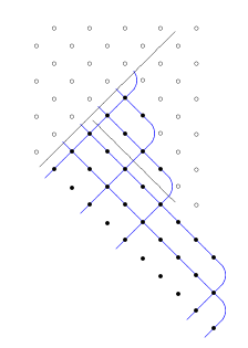
Figure 6. Cross-diagonals

In region $\mathfrak{2}$ and in the feasible subregion of region $\mathfrak{3}$, we insert into valley diagonal $i$ exactly $\nu(v,t)_{i}-\eta(v,t)_{i}$ zero-defects in the lowest cross-diagonal entries of the valley diagonal. (Observe that by definition, $\nu(v,t)_{i}-\eta(v,t)_{i}\leq r(v)$ for all $i$.) We also insert row $i$ of $\eta(v,t)$ as a consecutive sequence of one-defect ${\ast}$ entries lying on a diagonal emanating to the southeast from the top entry in valley diagonal $i$ not lying in region $\mathfrak{1}$.

Table 1 summarizes how the partitions are inserted into the regions.

Table 1. Partition insertion

$\lambda^{\dagger}_{i}$, $\lambda_{i}^{\prime}$	$\min(\lambda(v,t)^{\dagger}_{i},i-1)$ inserted as a consecutive NW-SE row of zero-defects on valley diagonal $i$; this is equivalent to inserting $\lambda_{i}^{\prime}$ as a column of zero-defects	region $\mathfrak{1}$
$\nu_{i}$	inserted as defects on the $i$th valley diagonal; • $\eta_{i}$ of these are one-defects lying at the top of the diagonal • $\nu_{i}-\eta_{i}\leq r(v)$ of these are zero-defects lying at cross-diagonal positions.	region $\mathfrak{2}$ and feasible subregion of $\mathfrak{3}$
	also inserted as a consecutive SW-NE row of plain-one entries	region $\mathfrak{1}$
$\eta_{i}$	inserted as a consecutive NW-SE row of one-defect entries along valley diagonal $i$ (followed by a single zero-defect)	region $\mathfrak{2}$ and feasible subregion of $\mathfrak{3}$
	also inserted as a consecutive NW-SE row of mask-value 1 entries defining the feasible subregion	region $\mathfrak{3}$

Figure 7. Some mask assignments for $r=3$

Example 4.5.

Figure 7 illustrates the construction for some typical partitions and $r=3$. Observe that each of the partitions $\lambda(v,t)^{\dagger}$, $\lambda^{\prime}(v,t)$, $\nu(v,t)$ and $\eta(v,t)$ are clearly embedded inside the heap.

Lemma 4.6.

The construction of $\sigma(t)$ is consistent in the sense that valley diagonal $i$ always has at least $\nu(v,t)_{i}-\eta(v,t)_{i}$ cross-diagonal entries. Furthermore, the $i$th valley diagonal in $\sigma(t)$ contains exactly $\lambda(v,t)^{\dagger}_{i}$ defects.

Proof.

First, suppose that $\eta(v,t)_{i}\neq 0$. Then, the lowest one-defect $p$ on valley diagonal $i$ has a corresponding entry $q$ in the feasible subregion of region $\mathfrak{3}$ located exactly $r(v)$ diagonals to the NE, and $q$ has mask-value 1. Therefore, there exist by construction at least $r(v)\geq\nu(v,t)_{i}-\eta(v,t)_{i}$ cross-diagonal entries below $p$ on valley diagonal $i$.

Next, suppose that $j$ is the first diagonal having $\eta(v,t)_{j}=0$, so $\eta(v,t)_{i}\neq 0$ for all $i<j$. Then, for each $i\geq j$, we insert into valley diagonal $i$ precisely $\min(\lambda(v,t)^{\dagger}_{i},i-1)$ zero-defects in region $\mathfrak{1}$ together with $\nu(v,t)_{i}$ zero-defects in region $\mathfrak{2}$ or the feasible subregion of region $\mathfrak{3}$.

By construction, there exist $r(v)$ cross-diagonal entries in valley diagonal $j$. As we move one diagonal to the right, we lose one cross-diagonal entry. However, we gain a potential zero-defect position in region $\mathfrak{1}$, so the partition inequality $\lambda(v,t)^{\dagger}_{i+1}\leq\lambda(v,t)^{\dagger}_{i}$ implies that $\nu(v,t)_{i}$ decreases by at least 1. Hence, we always have enough cross-diagonal entries to insert into by induction.

Note that although our construction may require changing some of the mask-value 1 entries in the feasible subregion of region $\mathfrak{3}$ to be one-defects, we never change any of the entries outside of the feasible subregion in region $\mathfrak{3}$ because $\eta(v,t)$ is a partition.

Finally, it follows from the definitions that the $i$th valley diagonal in $\sigma(t)$ contains exactly $\lambda(v,t)^{\dagger}_{i}$ defects, because we insert $\min(\lambda(v,t)^{\dagger}_{i},i-1)$ zero-defects in region $\mathfrak{1}$ together with $\nu(v,t)_{i}$ total defects below region $\mathfrak{1}$. Hence, we insert $\lambda(v,t)^{\dagger}_{i}$ defects in all. ∎

Lemma 4.7.

Each entry in $\sigma(t)$ restricted to the current segment has the defect status that we claimed in the construction, and $\mathsf{w}^{\sigma(t)}=x(t)$. Furthermore, the construction preserves the mask-value and defect status of all entries outside the current segment.

Proof.

We work by induction on the number of entries in $\lambda(v,t)^{\dagger}$. The base case is when $\lambda(v,t)^{\dagger}=\emptyset$, which corresponds to the mask $\gamma(t)$.

Since $v$ and $t$ will be fixed throughout the proof, we sometimes omit these arguments from the partitions $\lambda^{\dagger}$, $\nu$ and $\eta$. Also, we denote $\sigma(t)$ restricted to the current segment by $\sigma(\lambda^{\dagger})$. To begin our proof of the inductive case, suppose the mask $\sigma(\lambda^{\dagger})$ is constructed as in the definition, all of the entries have the correct defect status, and the mask restricted to the current segment encodes the element obtained by restricting $x(t)$ to the current segment.

We now consider adding an entry $b$ at the end of row $i$ and hence in column $j=\lambda^{\dagger}_{i}+1$ of $\lambda^{\dagger}$. Row $i$ of $\lambda^{\dagger}$ containing $b$ corresponds to the valley diagonal $i$ in the heap. There are three cases:

1. Adding $b$ to $\lambda^{\dagger}$ does not change $\nu$ nor $\eta$.

2. Adding $b$ to $\lambda^{\dagger}$ adds an entry to $\nu$ but not $\eta$.

3. Adding $b$ to $\lambda^{\dagger}$ adds an entry to both $\nu$ and $\eta$.

Denote the result of adding $b$ to $\lambda^{\dagger}$, $\nu$, and $\eta$ respectively by $\widetilde{\lambda^{\dagger}}$, $\widetilde{\nu}$, and $\widetilde{\eta}$. We consider each case in turn.

Case (1). In this case, $\sigma(\widetilde{\lambda^{\dagger}})$ is obtained from $\sigma(\lambda^{\dagger})$ by adding a defect to column $v+j$ of the $i$th valley diagonal in region $\mathfrak{1}$, and the entries in regions $\mathfrak{2}$ and $\mathfrak{3}$ all remain the same.

First, we claim that $\nu_{j}>0$, so some entry in column $v+j$ has mask-value 1 in $\sigma(\lambda^{\dagger})$. To see this, consider that $b$ is inserted into row $i$ and column $j$ of $\lambda^{\dagger}$ with $j<i$. Otherwise, adding $b$ would have changed $\nu$. Hence, $\lambda^{\dagger}_{j}\geq j$, so $\nu_{j}>0$.

By the induction hypothesis, we have that $\sigma(\widetilde{\lambda^{\dagger}})$ is obtained from $\sigma(\lambda^{\dagger})$ by first shifting all of the entries of $\nu_{j}$ up one level in their columns of the heap in region $\mathfrak{1}$, then changing the entry $b$ that was the start of $\nu_{j}$ in $\sigma(\lambda^{\dagger})$ to be a zero-defect in $\sigma(\widetilde{\lambda^{\dagger}})$.

The schematic shown in Figure 8 shows how to move a single row of $\nu$ up one level in the heap using string moves. Here, a string move is an operation on masks in which we change the mask values of two entries $\{\sigma_{p},\sigma_{q}\}$ in the heap whose strings meet. The mask values $\sigma_{p}$ and $\sigma_{q}$ are replaced by $1-\sigma_{p}$ and $1-\sigma_{q}$ respectively, and no other mask-values are changed. Observe that each of these string moves preserves the element being encoded by the mask as well as the defect-status of the other entries in the heap.

$\rightarrow$

$\rightarrow$

Figure 8. Case (1) of the proof

Case (2). In this case, we add $b$ as a zero-defect to region $\mathfrak{2}$ or $\mathfrak{3}$. Abusing notation, let $b$ denote the lowest cross-diagonal entry on valley diagonal $i$ that is not a zero-defect. By the induction hypothesis, we have that $\sigma(\widetilde{\lambda^{\dagger}})$ is obtained from $\sigma(\lambda^{\dagger})$ by changing $b$ from a plain-one to a zero-defect and adding an additional plain-one at the end of $\nu_{i}$ in region $\mathfrak{1}$.

We claim that both of these can be accomplished with a single string move. To see this, observe that the right string of $b$ does not meet any mask-value 0 entries in region $\mathfrak{2}$ because as we move right, we lose a cross-diagonal entry and gain an entry from region $\mathfrak{1}$ on the valley diagonal, so the level of the highest cross-diagonal entry that is a zero-defect is strictly decreasing. By the definition, the right string emanating up from a cross-diagonal entry eventually hits a plain-zero in region $\mathfrak{3}$ and turns towards the northwest, following a column of $\eta$. Observe that the total number of valley diagonals crossed by the right string is equal to the number of zero-defects in row $i$ of $\nu$ by the definition because all of the rowlengths in $\eta$ are distinct by Lemma 4.4. Hence, we have that the right string of $b$ meets the plain-zero $a$ that occurs just after the last entry in row $i$ of $\nu$ in region $\mathfrak{1}$.

The left string of $b$ emanates up towards the northwest and by induction eventually meets row $\nu_{i}$ in region $\mathfrak{1}$. Hence, the left and right strings of $b$ meet at the mask-value 0 entry $a$ just beyond the last entry in $\nu_{i}$. This is illustrated in Figure LABEL:f:c2. If we apply a string move to $b$ and $a$, we achieve the desired effect.

$\rightarrow$