Mechanical stiffening, bistability, and bit operations in a microcantilever

Abstract

We investigate the nonlinear dynamics of microcantilevers. We demonstrate mechanical stiffening of the frequency response at large amplitudes, originating from the geometric nonlinearity. At strong driving the cantilever amplitude is bistable. We map the bistable regime as a function of drive frequency and amplitude, and suggest several applications for the bistable microcantilever, of which a mechanical memory is demonstrated.

Microcantilevers are widely applied as transducers in sensitive instrumentation Rugar et al. (2004); Bleszynski-Jayich et al. (2009), with scanning probe microscopy as a clear example. Typically, the cantilever is operated in the linear regime, i.e. it is driven by a harmonic force at moderate strength, and its response is modulated by the parameter to be measured. In clamped-clamped mechanical resonators, additional applications have been proposed based on nonlinear behavior. Nonlinearity in clamped-clamped resonators is due to the extension of the beam, which results in frequency pulling and bistability at strong driving, and can be described by a Duffing equation Kozinsky et al. (2006). Applications which employ this bistability are e.g. elementary mechanical computing functions Badzey et al. (2004); Mahboob and Yamaguchi (2008). Since a cantilever beam is clamped only at one side, it can have a nonzero displacement without extending. One would therefore not expect a Duffing-like behavior for a cantilever beam. Nonlinear effects of a different origin have been observed in scanning probe microscopy, due to interactions between the cantilever and its environment. Tip-sample interactions either weaken or stiffen the cantilever response, depending on the strength of the softening Van der Waals forces and electrostatic interactions and the hardening short range interactions Rutzel et al. (2003); M$\mathrm{\ddot{u}}$ller et al. (1999). Weakening also occurs when the cantilever is driven by an electrostatic force Kacem et al. (2010). Besides nonlinear interactions with the environment, theoretical studies predict intrinsic nonlinear behavior of cantilever beams Crespo da Silva and Glynn (1978a, b); Nayfeh and Mook (1995); Mahmoodi and Jalili (2007); Kacem et al. (2010) , of which indications have been reported Mahmoodi and Jalili (2007); Ono et al. (2008).
In this letter, we report a detailed experimental analysis on the nonlinear mechanics of microcantilevers. It is shown that a hardening geometric nonlinearity dominates over softening nonlinear inertia, which effectively leads to a stiffening frequency response for the fundamental mode. At large amplitudes, the mechanical stiffening results in frequency pulling and ultimately in intrinsic bistability of the cantilever. We study the bistability in detail by measuring the cantilever response as a function of the frequency and amplitude, and compare the experimental observations with theory. A good agreement is found. We suggest several applications for the bistable cantilever, and as an example we demonstrate that bit operations can be implemented in the bistable cantilever.

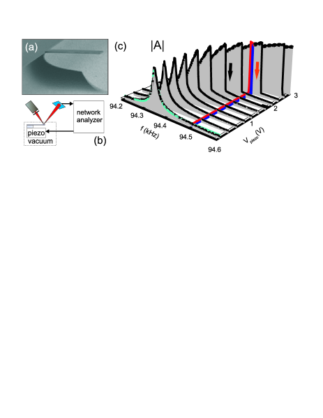
Figure 1: (a) Scanning electron micrograph of a silicon nitride cantilever; (b) Experimental setup; (c) Response lines for several drive voltages (forward frequency sweeps). A damped driven harmonic oscillator fit is shown for the weakly driven cantilever. The line at $\mathrm{f=94.5kHz}$ represents a response along the (decreasing) drive strength axis. The arrows indicate the switching direction.

Experiments are performed on thin cantilevers with a rectangular cross section, $\mathrm{w\times h}$, fabricated from low-pressure chemical vapor deposited silicon nitride using electron beam lithography and an isotropic reactive ion etching release process. Figure 1 (a) shows a scanning electron micrograph of a fabricated cantilever. The cantilever is mounted on a piezo actuator and placed in a vacuum chamber at a pressure of $\sim 10^{-4}$ mbar. At this pressure, the cantilever operates in the intrinsic damping regime. An optical deflection technique is deployed to detect the displacement of the driven cantilever, and the frequency response is measured using a network analyzer, see Fig. 1(b).
Figure 1 (c) shows frequency response lines for a weakly and strongly driven cantilever with length $\mathrm{L=40\;\mu m}$ and $\mathrm{w\times h=8\;\mu m\times 200\;nm}$. For weak driving the response fits a damped driven harmonic oscillator, with $\mathrm{f_{0}=94.35}$ kHz and $\mathrm{Q\approx 3000}$. Figure 1(c) also shows the response when driven at increasing strength: the resonance peak shifts to a higher value and the response becomes bistable. It resembles the response of a clamped-clamped beam driven in the nonlinear regime. A more detailed measurement is presented in Fig. 2(a,b). Here the magnitude of the resonator response, $|A|$, is depicted (color scale) as a function of the drive frequency and strength. The frequency is swept forward (i.e. from a low to a high frequency, FW) and backward (BW), and after each frequency response measurement the drive strength is increased. Parameters which result in a hysteretic (HY) response are visualized by subtracting forward and backward traces, as shown in Fig. 2(c).

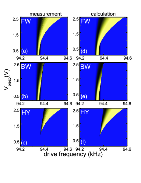
Figure 2: FIG. 2. Frequency pulling and bistability in a cantilever, measurement (left) and calculation by solving Eq. 3 (right). The color scale represents the magnitude of the frequency response, $\mathrm{|A|}$. The drive frequency is swept from a low to a high value (a,d) and vice versa (b,e). Panels (c,f) show the bistable regime, obtained by subtracting the forward from the backward response. As the piezoelectric coupling parameter is not known, the y-axis in the calculations has been scaled to match the experimental values.

The theory of nonlinear oscillations of a cantilever beam has been developed in Refs. Crespo da Silva and Glynn (1978a, b). Using the extended Hamilton principle the equation of motion for the displacement $\tilde{u}$ is derived:

$$D[\tilde{u}^{\prime\prime\prime\prime}+[\tilde{u}^{\prime}(\tilde{u}^{\prime}\tilde{u}^{\prime\prime})^{\prime}]^{\prime}]+\rho wh\ddot{\tilde{u}}+\tilde{\eta}\dot{\tilde{u}}+\frac{1}{2}\rho wh\Big{(}\tilde{u}^{\prime}\int_{L}^{s}\frac{\partial^{2}}{\partial\tilde{t}^{2}}\int_{0}^{s_{1}}(\tilde{u}^{\prime})^{2}ds_{2}ds_{1}\Big{)}^{\prime}=\tilde{F}.$$ (1)

The dots and primes denote differentiation to time $\tilde{t}$ and the arc length $s$ of the cantilever respectively, and $D$ is the bending rigidity, $\rho$ the density, and $\tilde{\eta}$ is the damping parameter. The piezo actuator generates a displacement ${U}=d_{33}V\cos(\tilde{\Omega}t)$, where V is the drive voltage and $d_{33}$ the piezoelectric coefficient. The resulting force on the cantilever equals $\tilde{F}=\ddot{U}\rho wh=-\tilde{\Omega}^{2}\rho whd_{33}V\cos(\tilde{\Omega}t)$. Equation (1) is transformed to a dimensionless form by substituting $u=\tilde{u}/h$, $x=s/L$, $l=d_{33}V/h$, $\eta=\eta^{\prime}L^{4}/(D\tau)$ and $\delta=(h/L)^{2}$. The time $\tilde{t}$ and drive frequency $\tilde{\Omega}$ are scaled using $\tau=L^{2}\sqrt{\rho wh/D}$. Applying the Galerkin procedure Atluri (1973); Kacem et al. (2010) for the first mode ($u=a(t)\xi(x)$) gives:

$$\ddot{a}+\omega^{2}a+\eta\dot{a}+40.44\delta a^{3}+4.60\delta(a\dot{a}^{2}+a^{2}\ddot{a})=-0.78l\Omega^{2}\cos(\Omega t).$$ (2)

Here, $a$ is the normalized coordinate, and $\omega$ the dimensionless resonance frequency; for the first mode $\omega=3.52$. The cubic term in $a$ represents the hardening geometric nonlinearity, and the fifth term represents nonlinear inertia which softens the frequency response Kacem et al. (2010). The values 40.44, 4.60 and 0.78 are obtained by integrating the linear mode shapes, $\xi(x)$ int . Equation 2 can be solved using the method of averaging or the method of multiple scales Nayfeh and Mook (1995) and the amplitude, $A$, can be implicitly written as:

$$A=\frac{l\Omega^{2}}{\sqrt{6.57(15.16\delta A^{2}-\omega\Omega+\omega^{2}(1-1.15\delta A^{2}))^{2}+1.64\eta^{2}\omega^{2}}}.$$ (3)

This equation is solved self-consistently to obtain the resonator amplitude, which is normalized by the drive strength $l$ to obtain the frequency response. Using the experimentally obtained linear resonance frequency, Q-factor and the dimensions as input parameters, the frequency responses are calculated as a function of the drive strength. Figures 2 (d,e) show the simulated stable solutions, which correspond to the resonator response to a forward and backward frequency sweep. The model captures the observed behavior well, where the piezoelectric coupling parameter is the only free parameter. Both the calculations and the experiments indicate that the geometric nonlinearity dominates over the inertial nonlinearity. Analyzing Eq. (3) in detail shows that the nonlinearity depends on the modeshape, $\mathrm{\xi(x)}$, and the squared aspect ratio, $\delta$. For the fundamental mode, the intrinsic nonlinearity in cantilevers always leads to stiffening of the frequency response. In contrast, the calculation shows that the same nonlinearity results in a weakening effect for higher modes hig .
The intrinsic mechanical bistability allows cantilever applications similar to the ones implemented in clamped-clamped resonators. As an example, we demonstrate mechanical bit operations in a cantilever with dimensions $L\times w\times h=\,\mathrm{30\,\mu m\,\times\,8\,\mu m\,\times\,150}$ nm, with a linear resonance frequency $\mathrm{f_{0}=193.49}$ kHz and $\mathrm{Q\approx 5800}$ in vacuum. For this cantilever, a measurement of the hysteretic regime is shown in Fig 3 (a) pie . Bit operations can be performed by modulating the drive frequency or the drive strength –or a combination thereof– across the hysteretic regime, a scheme that was also deployed to implement nanomechanical memory in clamped-clamped beams Badzey et al. (2004); Mahboob and Yamaguchi (2008). The principle is indicated by the arrows in Fig. 3(a). The drive strength is modulated by varying the voltage on the piezo at a fixed frequency, as shown in Fig. 3(b). A backward sweep in the drive strength follows the high-amplitude state, similar to a forward sweep in drive frequency. This intuitively becomes clear in Fig. 1(c), where the transition from a high to a low amplitude occurs during a backward sweep in the drive strength, as indicated by the red line along the fixed frequency at $\mathrm{f=94.5kHz}$. During a forward sweep in the drive strength the resonator follows the low-amplitude stable branch, as with a backward sweep in frequency.

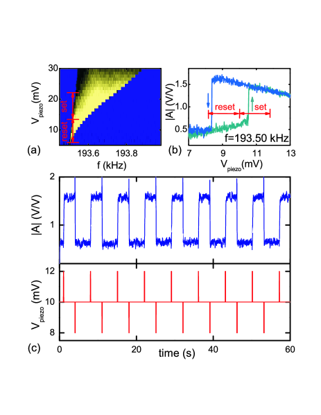
Figure 3: Hysteretic regime for a $\mathrm{30\;\mu m\times 8\;\mu m\times 150\;nm}$ cantilever. (b) Drive strength sweep at fixed frequency, and indication of the modulation to implement the bit. (c) Mechanical memory in a bistable cantilever beam: drive strength (lower panel) and cantilever response (upper panel).

To implement the bit, the cantilever is driven in the bistable regime at $\mathrm{f=193.50\;kHz}$ and $\mathrm{V_{piezo}=10\;mV}$. To set and reset the cantilever bit, the drive voltage is modulated by 2 mV around the operating point, as indicated by the arrows in Fig. 3(b). Starting at low amplitude, ’0’ in Fig. 3(c), a high-amplitude ’1’ is written by temporary increasing the drive voltage to 12 mV. The cantilever switches to a high vibrational amplitude and remains in this state after the drive voltage is set back to the operating point. Next, the drive strength is lowered to 8 mV which resets the cantilever to a low amplitude oscillation, corresponding to ’0’.
Bistability of cantilever beams can be used for various purposes besides the mechanical memory application described here. For example, the hysteretic frequency response facilitates the readout of cantilever arrays in dissipative environments by employing the scheme described earlier Venstra and van der Zant (2008). Bistability may also open the way to use a cantilever as its own bifurcation amplifier Greywall et al. (1994); Siddiqi et al. (2004); Gammaitoni et al. (1998); Almog et al. (2007) in for example scanning probe microscopy, thereby enhancing the sensitivity to external stimuli. Finally, we note that despite scaling with the aspect ratio squared, $\delta$, the bistable regime is also accessible for single-clamped nanoscale resonators such as carbon nanotubes Perisanu et al. (2010).
In conclusion, we investigated the nonlinear oscillations of microcantilever beams. Mechanical stiffening is observed which results in frequency pulling and bistability. The experiments are in excellent agreement with calculated nonlinear response. Several applications for the bistable cantilever are suggested, of which a mechanical memory is demonstrated.
The authors acknowledge Khashayar Babaei Gavan for fabricating the devices, and the Dutch organization FOM (Program 10, Physics for Technology) for financial support.

References

- Rugar et al. (2004) D. Rugar, R. Budakian, H. Mamin, and B. Chui, Nature 430, 329 (2004).
- Bleszynski-Jayich et al. (2009) A. C. Bleszynski-Jayich, W. E. Shanks, B. Peaudecerf, E. Ginossar, F. von Oppen, L. Glazman, and J. G. E. Harris, Science 326, 272 (2009).
- Kozinsky et al. (2006) I. Kozinsky, H. W. C. Postma, I. Bargatin, and M. L. Roukes, Appl. Phys. Lett. 88, 253101 (2006).
- Badzey et al. (2004) R. L. Badzey, G. Zolfagharkhani, A. Gaidarzhy, and P. Mohanty, Appl. Phys. Lett. 85, 3587 (2004).
- Mahboob and Yamaguchi (2008) I. Mahboob and H. Yamaguchi, Nature Nanotech. 3, 275 (2008).
- Rutzel et al. (2003) S. Rutzel, S. Lee, and A. Raman, Proc. R. Soc. London Ser. A-Math. Phys. Eng. Sci. 459 (2003).
- Mller et al. (1999) D. Mller, D. Fotiadis, S. Scheuring, S. Mller, and A. Engel, Biophys. J. 76, 1101 (1999).
- Kacem et al. (2010) N. Kacem, J. Arcamone, F. Perez-Murano, and S. Hentz, J. Micromech. Microeng. 20 (2010).
- Crespo da Silva and Glynn (1978a) M. R. M. Crespo da Silva and C. C. Glynn, J. Struct. Mech. 6 (1978a).
- Crespo da Silva and Glynn (1978b) M. R. M. Crespo da Silva and C. C. Glynn, J. Struct. Mech. 6 (1978b).
- Nayfeh and Mook (1995) A. H. Nayfeh and D. T. Mook, Nonlinear Oscillations (Wiley, 1995).
- Mahmoodi and Jalili (2007) S. N. Mahmoodi and N. Jalili, Int. J. of Nonlin. Mech. 42, 577 (2007).
- Ono et al. (2008) T. Ono, Y. Yoshida, Y.-G. Jiang, and M. Esashi, Appl. Phys. Express 1 (2008).
- Atluri (1973) S. Atluri, J. Appl. Mech.-Trans. ASME 40, 121 (1973).
- (15) The prefactors in Eq. 2 are calculated by integrating the modeshapes and their derivatives as follows: , and .
- (16) For the four lowest flexural modes, the prefactors in Eq.2 are 40.44066, 13418.09, 264384.7, and 1916632 for the geometry, 4.596772, 144.7255, 999.9000, and 3951.323 for the nonlinear inertia, and 0.782992, 0.433936, 0.254430, and 0.181627 for the force. The dimensionless frequencies are 3.516015, 22.03449, 61.69721, and 120.9019. These values yield a stiffening frequency response of the fundamental mode, and a weakening one for the second, third, and fourth flexural mode.
- (17) A different piezo actuator is used in this experiment.
- Venstra and van der Zant (2008) W. J. Venstra and H. S. J. van der Zant, Appl. Phys. Lett. 93, 234106 (2008).
- Greywall et al. (1994) D. S. Greywall, B. Yurke, P. A. Busch, A. N. Pargellis, and R. L. Willet, Phys. Rev. Lett. 72, 2992 (1994).
- Siddiqi et al. (2004) I. Siddiqi, R. Vijay, F. Pierre, C. Wilson, M. Metcalfe, C. Rigetti, L. Frunzio, and M. Devoret, Phys. Rev. Lett. 93 (2004).
- Gammaitoni et al. (1998) L. Gammaitoni, P. Hanggi, P. Jung, and F. Marchesoni, Rev. Mod. Phys. 70, 223 (1998).
- Almog et al. (2007) R. Almog, S. Zaitsev, O. Shtempluck, and E. Buks, Appl. Phys. Lett. 90 (2007).
- Perisanu et al. (2010) S. Perisanu, T. Barois, A. Ayari, P. Poncharal, M. Choueib, S. T. Purcell, and P. Vincent, Phys. Rev. B 81 (2010).