Unified description of quark and lepton mixing matrices based on a Yukawaon model

Abstract

Based on a supersymmetric Yukawaon model with O(3) family symmetry, possible forms of quark and lepton mixing matrices are systematically investigated under a condition that the up-quark mass matrix form leads to the observed nearly tribimaximal mixing in the lepton sector. Although the previous model could not provide a good fitting of the observed quark mixing, the present model can give a reasonably good fitting not for lepton mixing but also the quark mixing by using a different origin of the $CP$ violation from one in the previous model.

I Introduction

One of the current subjects of the particle flavor physics is to understand quark and lepton masses and mixings. The investigation of them, even if it is phenomenological, will provide a promising clue to new physics. The so-called “tribimaximal” mixing observed in the neutrino mixing atm ; solar is very suggestive of a fundamental law in the lepton sector. Usually, the observed tribimaximal mixing has been explained by assuming a discrete symmetry tribi .

Meanwhile, as a neutrino mass matrix model without assuming any discrete symmetry, an unfamiliar model MNS_yukawaon08 ; O3PLB09 has been proposed by using a seesaw type neutrino mass matrix $M_{\nu}=m_{D}M_{R}^{-1}m_{D}^{T}$. In this model, the Dirac neutrino mass matrix $m_{D}$ is given by $m_{D}\propto M_{e}$ ($M_{e}$ is a charged lepton mass matrix) and the Majorana mass matrix $M_{R}$ of the right-handed neutrinos is given by

$$M_{R}\propto M_{u}^{1/2}M_{e}+M_{e}M_{u}^{1/2}.$$

Here $M_{u}^{1/2}$ is defined by $M_{u}^{1/2}(M_{u}^{1/2})^{T}=M_{u}$ ($M_{u}$ is an up-quark mass matrix with a symmetric form $M_{u}^{T}=M_{u}$). The model O3PLB09 can lead to a nearly tribimaximal mixing by assuming suitable up-quark mass matrix as we give a short review in the next section. The model has only four parameters: one ($\xi_{\nu}$) is in the neutrino sector, and one ($a_{u}$) is in the up-quark sector, and two ($a_{d}e^{i\alpha_{d}}$) in the down-quark sector. (Here, we consider that the charged lepton mass $(m_{e},m_{\mu},m_{\tau})$ are known parameters, and we do not count these parameters as adjustable parameters.) This model leads to excellent fitting for up-quark mass ratios $m_{u}/m_{c}$ and $m_{c}/m_{t}$ and neutrino mixing parameters $\sin^{2}2\theta_{atm}$, $\tan^{2}\theta_{solar}$ and $|U_{e3}|^{2}$, only by adjusting the two parameters $a_{u}$ and $\xi_{\nu}$. On the other hand, for down-quark sector, the fitting is not so excellent, especially, the predicted values of $|V_{ub}|$ and $|V_{td}|$ are somewhat large compared with the observed values as far as we use parameter values which can give reasonable values for the observed down-quark mass ratios.

The purpose of the present paper is to investigate an improved version of the above model and to search systematically for parameter values which can give reasonable quark mass ratios, quark mixing parameters (Cabibbo-Kobayashi-Maskawa (CKM) mixing matrix) and neutrino mixing parameters. In Sec.II, we will show that the four parameter model cannot have reasonable parameter region consistent with four quark mass ratios, three neutrino mixing parameters, and four CKM mixing parameters. In Sec.III, we propose a revised model and give parameter fitting for 11 observables. (In the present model, we do not discuss the observed value $R\equiv\Delta m^{2}_{solar}/\Delta m^{2}_{atm}$ for neutrino masses, because we can always have an additional one parameter which inevitably appears in the model and affects only the mass ratios $R$, but does not affect neutrino mixing and observables in the quark sector.) Finally, Sec.IV is devoted to the summary and discussions.

II Supersymmetric Yukawaon model

In this section, we give a short review of a quark and lepton mass matrix model O3PLB09 based on the supersymmetric Yukawaon model, because, in this paper, we propose a revised version of this model.

In the Yukawaon model, we put the following assumption:

(i) We consider that the Yukawa coupling constants are effectively given by

$$Y_{f}^{eff}=y_{f}\frac{\langle Y_{f}\rangle}{\Lambda},$$

where $\langle Y_{f}\rangle$ ($f=u,d,e,\nu$ and so on) are vacuum expectation values (VEVs) of new scalars $Y_{f}$ with $3\times 3$ components of O(3) family symmetry and $\Lambda$ is an energy scale of the effective theory. (For the time being, we assume $\Lambda\sim 10^{14-15}$ GeV.) Therefore, the would-be Yukawa interactions are given by

$$H_{Y}=\sum_{i,j}\frac{y_{u}}{\Lambda}u^{c}_{i}(Y_{u})_{ij}{q}_{j}H_{u}+\sum_{i,j}\frac{y_{d}}{\Lambda}d^{c}_{i}(Y_{d})_{ij}{q}_{j}H_{d}$$

$$+\sum_{i,j}\frac{y_{\nu}}{\Lambda}\ell_{i}(Y_{\nu})_{ij}\nu^{c}_{j}H_{u}+\sum_{i,j}\frac{y_{e}}{\Lambda}\ell_{i}(Y_{e})_{ij}e^{c}_{j}H_{d}+{\rm H.c.}+\sum_{i,j}y_{R}\nu^{c}_{i}(Y_{R})_{ij}\nu^{c}_{j},$$

where $q$ and $\ell$ are SU(2)_L doublet fields, and $f^{c}$ ($f=u,d,e,\nu$) are SU(2)_L singlet fields.

(ii) In order to distinguish each $Y_{f}$ from others, we assume a U(1)_X symmetry (i.e. “sector charge”) in addition to the O(3) symmetry, and we have assigned U(1)_X charges as $Q_{X}(Y_{f})=x_{f}$, $Q_{X}(f^{c})=-x_{f}$ and $Q_{X}(Y_{R})=2x_{\nu}$. (The SU(2)_L doublet fields $q$, $\ell$, $H_{u}$ and $H_{d}$ are assigned to sector charges $Q_{X}=0$.)

(iii) For the neutrino sector, we assume $Q_{X}(\nu^{c})=Q_{X}(e^{c})$, so that the Yukawaon $Y_{e}$ can also couple to the neutrino sector as $(\ell Y_{e}\nu^{c})H_{u}$ instead of $(\ell Y_{\nu}\nu^{c})H_{u}$ in Eq.(2.2). Therefore, we can change the above model into a model without $Y_{\nu}$. Hereafter, we read $Y_{\nu}$ in Eq.(2.2) as $Y_{e}$. Besides, we can have a term

$$\sum_{i,j,k}\frac{y^{\prime}_{R}}{\Lambda}\nu^{c}_{i}(Y_{e})_{ik}(Y_{e})_{kj}\nu^{c}_{j},$$

in addition to the right-hand side of Eq.(2.2), because $Y_{e}Y_{e}$ has the same U(1)_X charge as $Y_{R}$, i.e. $Q_{X}=2x_{e}$. Although this term (2.3) leads to an additional neutrino mass term, the term does not affect neutrino mixing inverseM_nu as far as the neutrino mass matrix $M_{\nu}$ is real, because of $M_{\nu}\propto Y_{e}[(\cdots)+Y_{e}Y_{e}]^{-1}Y_{e}=[Y_{e}^{-1}(\cdots)Y_{e}^{-1}+{\bf 1}]^{-1}$.

(iv) We give a superpotential $W$ which is invariant under O(3) family symmetry and U(1)_X symmetry, and solve supersymmetric (SUSY) vacuum conditions. As a result, we obtain VEV relations among Yukawaons.

For example, we have assumed the following superpotential

$$W_{e}=\lambda_{e}{\rm Tr}[\Phi_{e}\Phi_{e}\Theta_{e}]+\mu_{e}{\rm Tr}[Y_{e}\Theta_{e}]+W_{\Phi}.$$

Here we have assumed $Q_{X}(\Phi_{e})=\frac{1}{2}Q_{X}(Y_{e})=-\frac{1}{2}Q_{X}(\Theta_{e})$ and the term $W_{\Phi}$ has been introduced in order to determine a VEV spectrum $\langle\Phi_{e}\rangle$ completely. Then, from a SUSY vacuum condition

$$\frac{\partial W}{\partial\Theta_{e}}=\lambda_{e}\Phi_{e}\Phi_{e}+\mu_{e}Y_{e}=0,$$

we obtain a VEV relation

$$\langle Y_{e}\rangle=-\frac{\lambda_{e}}{\mu_{e}}\langle\Phi_{e}\rangle\langle\Phi_{e}\rangle.$$

The VEV value $\langle\Phi_{e}\rangle$ is derived from the term $W_{\Phi}$ (for example, see Refs.Sumino09PLB ; Sumino09JHEP ; e-spec_10PLB ). However, for simplicity, in this paper, we use the observed values of the charged lepton masses straightforwardly for the VEV value as given by

$$\langle\Phi_{e}\rangle_{e}={\rm diag}(v_{1},v_{2},v_{3})\propto{\rm diag}(\sqrt{m_{e}},\sqrt{m_{\mu}},\sqrt{m_{\tau}}).$$

In other words, we have assumed the ad hoc relation (2.7), the derivation of which is not discussed in the present paper. Hereafter, for counting a number of “adjustable” parameters, we do not include $v_{i}$ in the number. Here, the notation $\langle A\rangle_{f}$ denotes a form of a VEV matrix $\langle A\rangle$ in the diagonal basis of $\langle Y_{f}\rangle$ (we refer to it as $f$ basis). The scalar $\Theta_{e}$ does not have a VEV, i.e. $\langle\Theta_{e}\rangle=0$. Therefore, terms which include more than two of $\Theta_{e}$ do not play any physical role, so that we do not consider such terms in the present effective theory. [Hereafter, we will denote fields whose VEV values are zero as notations $\Theta_{A}$ ($A=u,d,\cdots$).]

Next, for the purpose of the comparison of our new model with the previous one, we give a short review of quark and lepton mass matrix forms of the previous model discussed in Ref.O3PLB09 . The explicit form of the superpotential for the previous model is given in Ref.O3PLB09 . That, for the new model, shall be given in the next section.

In the previous modelO3PLB09 , the quark mass matrices, i.e. $\langle Y_{u}\rangle$ and $\langle Y_{d}\rangle$, are given as

$$M_{u}\propto\langle Y_{u}\rangle\propto\langle\Phi_{u}\rangle\langle\Phi_{u}\rangle,$$

$$\langle\Phi_{u}\rangle_{e}\propto\langle\Phi_{e}\rangle_{e}\left(\langle E\rangle_{e}+a_{u}\langle X\rangle_{e}\right)\langle\Phi_{e}\rangle_{e},$$

$$M_{d}\propto\langle Y_{d}\rangle_{e}\propto\langle\Phi_{e}\rangle_{e}\left(\langle E\rangle_{e}+a_{d}e^{i\alpha_{d}}\langle X\rangle_{e}\right)\langle\Phi_{e}\rangle_{e},$$

respectively. (For convenience, we have changed the definitions of $a_{u}$ and $a_{d}$ from those in Ref.O3PLB09 .) Here, $\langle X\rangle_{e}$ and $\langle E\rangle_{e}$ are given by

$$\langle X\rangle_{e}=Xv_{X}\equiv\frac{1}{3}\left(\begin{array}[]{ccc}1&1&1\\ 1&1&1\\ 1&1&1\end{array}\right)v_{X},\ \ \ \ \ \langle E\rangle_{e}={\bf 1}v_{E}\equiv\left(\begin{array}[]{ccc}1&0&0\\ 0&1&0\\ 0&0&1\end{array}\right)v_{E}.$$

(Here, the VEV form $\langle X\rangle_{e}$ breaks the O(3) flavor symmetry into S₃.) Therefore, we obtain quark mass matrices

$$M_{u}^{1/2}\propto M_{e}^{1/2}\left({\bf 1}+a_{u}{X}\right)M_{e}^{1/2},\ \ \ M_{d}\propto M_{e}^{1/2}\left({\bf 1}+a_{d}e^{i\alpha_{d}}{X}\right)M_{e}^{1/2},$$

on the $e$ basis. Here, we have redefined the coefficients $a_{u}v_{X}/v_{E}$ and $a_{d}v_{X}/v_{E}$ in Eqs.(2.9) and (2.10) as $a_{u}$ and $a_{d}$, respectively. Hereafter, for numerical estimate of $a_{u}$ and $a_{d}$, we use the definition of those in Eq.(2.12). (This quark mass matrix form (2.12) has first been proposed in Ref.DemocSeesaw as a “democratic universal seesaw mass matrix model”.) Note that we have assumed that the O(3) relations are valid only on the $e$ and $u$ bases, so that $\langle Y_{e}\rangle$ and $\langle Y_{u}\rangle$ must be real. [The VEV matrix $\langle\Phi_{u}\rangle$ must satisfy the relation (2.9) on the $e$ basis, while $\langle\Phi_{u}\rangle$ must also satisfy the relation $\langle Y_{u}\rangle\propto\langle\Phi_{u}\rangle_{u}\langle\Phi_{u}\rangle_{u}$ on the $u$ basis. However, for the down-quark sector, such a condition is not required, because $\langle Y_{d}\rangle$ is given by Eq.(2.10) only on the $e$ basis.]

A case $a_{u}\simeq-1.79$ can give a reasonable up-quark mass ratios $\sqrt{{m_{u1}}/{m_{u2}}}=0.043$ and $\sqrt{{m_{u2}}/{m_{u3}}}=0.057$, which are in favor of the observed values q-mass

$$\sqrt{\frac{m_{u}}{m_{c}}}=0.045^{+0.013}_{-0.010},\ \ \ \ \sqrt{\frac{m_{c}}{m_{t}}}=0.060\pm 0.005,$$

at $\mu=m_{Z}$.

In this paper, we will carry out parameter-fitting at $\mu=m_{Z}$, because we interest in the mixing values at $\mu=m_{Z}$. Exactly speaking, fitting for the mass ratios must be done at $\mu=\Lambda\sim 10^{14}$ GeV. However, at present, our model does not intend to give so precise predictions of the quark mass ratios. For example, we know q-mass $\sqrt{m_{u}/m_{c}}=0.046^{+0.013}_{-0.012}$ and $\sqrt{m_{c}/m_{t}}=0.051^{+0.002}_{-0.006}$ even at $\mu=2\times 10^{16}$ GeV ($\tan\beta=10$). Even in $\sqrt{m_{c}/m_{t}}$, the discrepancy is smaller than 20%. Besides, the mass values are dependent on the value of $\tan\beta$ in the SUSY model. Therefore, for simplicity, in this paper, we will carry out the parameter-fitting at $\mu=m_{Z}$.

On the other hand, in the neutrino mass matrix

$$M_{\nu}\propto\langle Y_{e}\rangle_{e}\langle Y_{R}\rangle_{e}^{-1}\langle Y_{e}\rangle_{e},$$

the Majorana mass matrix of the right-handed neutrinos $\langle Y_{R}\rangle_{e}$ is given by

$$\langle Y_{R}\rangle\propto\langle Y_{e}\rangle_{e}\langle P_{u}\rangle_{e}\langle\Phi_{u}\rangle_{e}+\langle\Phi_{u}\rangle_{e}\langle P_{u}\rangle_{e}\langle Y_{e}\rangle_{e}+\xi_{\nu}(\langle P_{u}\rangle_{e}\langle Y_{e}\rangle_{e}\langle\Phi_{u}\rangle_{e}+\langle\Phi_{u}\rangle_{e}\langle Y_{e}\rangle_{e}\langle P_{u}\rangle_{e}).$$

Here, we have introduced a new field $P_{u}$ with a VEV

$$\langle P_{u}\rangle_{u}\propto{\rm diag}(+1,-1,+1),$$

in order to make “effective” eigenvalues of $\langle\Phi_{u}\rangle_{u}$ positive, because the eigenvalues of $\langle\Phi_{u}\rangle_{u}=(v_{u1},v_{u2},v_{u3})$ give signs $(+,-,+)$ for the parameter value $a_{u}\sim-1.8$. (The field $P_{u}$ has been introduced from a phenomenological reason. If the factor (2.16) were absence [i.e. $Y_{R}$ were given by $\langle Y_{R}\rangle\propto\langle Y_{e}\rangle_{e}\langle\Phi_{u}\rangle_{e}+\langle\Phi_{u}\rangle_{e}\langle Y_{e}\rangle_{e}$], we could not give the observed maximal mixing $\sin^{2}2\theta_{atm}\simeq 1$ atm for any values of the parameters $a_{u}$ and $\xi_{\nu}$.) The reason for the $\xi_{\nu}$ term in Eq.(2.15) is as follows: When we consider a term $Y_{e}P_{u}\Phi_{u}+\Phi_{u}P_{u}Y_{e}$ we must also consider an existence of $P_{u}Y_{e}\Phi_{u}+\Phi_{u}Y_{e}P_{u}$ O3PLB09 , because they have the same U(1)_X charges. The results at $a_{u}\simeq-1.78$ are excellently in favor of the observed neutrino oscillation parameters $\sin^{2}2\theta_{atm}=1.00_{-0.13}$ atm and $\tan^{2}\theta_{solar}=0.469^{+0.047}_{-0.041}$ solar by taking a small value of $|\xi_{\nu}|$, $\xi_{\nu}=+0.005$ or $\xi_{\nu}=-0.0012$.

Thus, the model in Ref.O3PLB09 can successfully fit two up-quark mass ratios and three neutrino mixing parameters only by the two parameters $a_{u}$ and $\xi_{\nu}$. On the other hand, the fitting of six observable quantities (two down-quark mass ratios and four CKM mixing parameters) only by two parameters $a_{d}$ and $\alpha_{d}$ given in Ref.O3PLB09 are not in excellent agreement with the observed values. Especially, the predicted values of $|V_{ub}|$ and $|V_{td}|$ are considerably larger than the observed ones. We find from a systematical parameter search that this is not due to incompleteness of the parameter search, but plausible values of the CKM mixing parameters cannot be obtained even if we abandon the fitting of the down-quark mass ratios.

Considering the success in the up-quark and neutrino sectors, we do not change the model for the up-quark and neutrino sectors. We fix the parameter values as $a_{u}\sim-1.8$. The observed values of the down-quark masses are as follows q-mass

$${\frac{m_{d}}{m_{s}}}=0.053^{+0.051}_{-0.029},\ \ \ \ {\frac{m_{s}}{m_{b}}}=0.019\pm 0.006,$$

at $\mu=m_{Z}$. We consider that the mass ratio $m_{d}/m_{s}$ may be sensitive due to an unknown effect of a minor change of the model, so that, for the time being, we disregard the fitting of $m_{d}/m_{s}$ and concentrate on the fitting of $m_{s}/m_{b}$. Although a parameter value $a_{d}\sim-16$ can give a reasonable prediction of $m_{s}/m_{b}$, the solution cannot give reasonable predictions of the CKM mixing parameters, we rule out this solution $a_{d}\sim-16$. We find that there are another solutions of $a_{d}$ in a range $-a_{d}=1.3-1.7$, which can roughly give $m_{s}/m_{b}=0.1-0.4$. The solutions have a possibility that they can give reasonable values of the CKM mixing parameters. Therefore, we investigate the case with $-a_{d}=1.3-1.7$ in detail.

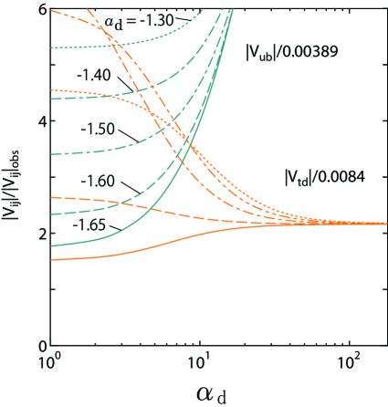
Figure 1: $|V_{ij}|/|V_{ij}|_{obs}$ versus a phase parameter $\alpha_{d}$. (a) $|V_{us}|/0.2252$ and $|V_{cb}|/0.0406$; (b) $|V_{ub}|/0.00389$ and $|V_{td}|/0.0084$. The parameter $a_{u}$ in the up-quark sector is fixed at $a_{u}=-1.79$. The five curves represent $a_{d}=-1.30$, $-1.40$, $-1.50$, $-1.60$ and $-1.65$, respectively.

The results are shown in Fig.1, where the predicted values $|V_{ij}|$ versus the phase parameter $\alpha_{d}$ are given in the unit of the observed values PDG10 $|V_{ij}|_{obs}$

$$\begin{array}[]{ll}|V_{us}|_{obs}=0.2252\pm 0.0009,&|V_{cb}|_{obs}=0.0406\pm 0.0013,\\ |V_{ub}|_{obs}=0.00389\pm 0.00044,&|V_{td}|_{obs}=0.0084\pm 0.0006.\end{array}$$

Here, we have illustrated the behaviors of $|V_{ij}|$ for the range $\alpha_{d}=0^{\circ}-180^{\circ}$, because the behaviors for $\alpha_{d}=360^{\circ}-180^{\circ}$ are just the same as that for $\alpha_{d}=0^{\circ}-180^{\circ}$. As seen in Fig.1(a), in order to obtain a reasonable value of $|V_{cb}|$, we must choose a value of $\alpha_{d}$ smaller than $\alpha_{d}\sim 10^{\circ}$, and also a value of $a_{d}$ smaller than $-a_{d}\sim 1.5$. However, from Fig.1(b), we can conclude there is no solution for a reasonable value of $|V_{us}|$ for any values of $a_{d}$ and $\alpha_{d}$ even at the cost of the fitting of down-quark mass ratios. Therefore, in the next section, we proposed a revised model for quark mass matrices keeping the model for the neutrino sectors.

III Phenomenology of quark mass matrices

We present an explicit form of the quark mass matrices in our new model. In this paper, we put the following assumptions for a phenomenological forms of quark mass matrices $M_{u}$ ($M_{u}^{1/2}$) and $M_{d}$:

(i) Differently from the previous model O3PLB09 , we regard that not only $\langle Y_{u}\rangle$ (also $\langle\Phi_{u}\rangle$) but also $\langle Y_{d}\rangle$ are real, i.e. $\alpha_{d}=0$ in Eq.(2.10). Instead, we consider that $CP$ violation in the quark sector originates in a phase matrix $\langle P_{d}\rangle_{e}=v_{Pd}P_{d}\equiv v_{Pd}{\rm diag}(e^{i\phi_{1}},e^{i\phi_{2}},e^{i\phi_{3}})$ which does not affect the down-quark mass ratios, but does only the CKM mixing. Namely the quark mass matrices $M_{u}^{1/2}$ and $M_{d}$ is given by

$$M_{u}^{1/2}\propto M_{e}^{1/2}({\bf 1}+a_{u}X)M_{e}^{1/2}+\xi_{u}\left(M_{e}^{1/2}M_{e}^{1/2}({\bf 1}+a_{u}X)+({\bf 1}+a_{u}X)M_{e}^{1/2}M_{e}^{1/2}\right)+m_{0u}{\bf 1},$$

$$M_{d}\propto P_{d}\left[M_{e}^{1/2}({\bf 1}+a_{d}X)M_{e}^{1/2}+\xi_{d}\left(M_{e}^{1/2}M_{e}^{1/2}({\bf 1}+a_{d}X)+({\bf 1}+a_{d}X)M_{e}^{1/2}M_{e}^{1/2}\right)+m_{0d}{\bf 1}\right]P_{d},$$

so that the CKM matrix $V$ is given by $V=R_{u}^{T}P_{d}R_{d}$, where $R_{u}$ and $R_{d}$ are defined by $R_{u}^{T}M_{u}^{1/2}R_{u}={\rm diag}(+\sqrt{m_{u}},-\sqrt{m_{c}},+\sqrt{m_{t}})$ (for $a_{u}\sim-1.8$) and $R_{d}^{T}(P_{d}^{\dagger}M_{d}P_{d}^{\dagger})R_{d}={\rm diag}(m_{d},m_{s},m_{b})$, respectively.

(ii) Similarly to Eq.(2.15), we assume the $\xi_{q}$ terms which originate in the reordering of the fields with the same quantum numbers.

(iii) Since only two of the three phase parameters $\phi_{1}$, $\phi_{2}$ and $\phi_{3}$ in the phase matrix $P_{d}={\rm diag}(e^{i\phi_{1}},e^{i\phi_{2}},e^{i\phi_{3}})$ are physically independent parameters. For convenience, we take $\phi_{3}=0$.

(iv) It is better that the parameter number is as few as possible. We consider that the first term is dominant in Eq.(3.1) [and also Eq.(3.2)], and we will consider $\xi_{q}$ and $m_{0q}$ terms as the need arises. As seen later, we can do fitting without $\xi_{d}$ and $m_{0u}$ terms.

Of course, we consider that these relations are derived from SUSY vacuum conditions for a given superpotential $W$. However, prior to investigating the superpotential form, from a phenomenological point of view, we would like to investigate whether there is a possible parameter region or not in the present model. A Yukawaon model for the phenomenological forms (3.1) and (3.2) will be discussed in the next section.

Since the mass spectra $M_{u}^{1/2}(a_{u})$ and $M_{d}(a_{d})$ have the same behavior for the parameter $a_{q}$ ($a_{u}$ and $a_{d}$), we illustrate the mass spectra versus $a_{q}$ in the limit of $\xi_{q}=0$ in Fig.2. (The mass values in Fig.2 read $(\sqrt{|m_{u}|},\sqrt{|m_{c}|},\sqrt{|m_{t}|})$ and $(|m_{d}|,|m_{s}|,|m_{b}|)$ for the up- and down-quark sectors, respectively.

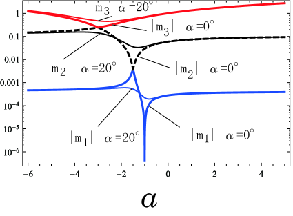
Figure 2: Eigenvalues $|m_{1}|,|m_{2}|,|m_{3}|$ versus a parameter $a$ in a mass matrix $M=M_{e}^{1/2}({\bf 1}+ae^{i\alpha}X)M_{e}^{1/2}$ with $\alpha=0$ (thick curves). For reference, a case with $\alpha=20^{\circ}$ is also illustrated by thin curves in the figure. $(|m_{1}|,|m_{2}|,|m_{3}|)$ read $(\sqrt{|m_{u}|}|,\sqrt{|m_{c}|},\sqrt{|m_{t}|})$ and $(|m_{d}|,|m_{s}|,|m_{b}|)$ for up- and down-quark sectors, respectively. Numerical values of the eigenvalues are given in a unit of $(m_{e}+m_{\mu}+m_{\tau})$.

In the present model, too, the model for the up-quark sector and neutrino sector is essentially unchanged from the previous model O3PLB09 except for the $\xi_{u}$ term given in (3.1). For reference, in Fig.3, we illustrate the up-quark mass ratios $\sqrt{m_{u}/m_{c}}$ and $\sqrt{m_{c}/m_{t}}$ versus $a_{u}$ and $\xi_{u}$. As seen in Fig.3, there are two set of the solution $(a_{u},\xi_{u})$ [regions (i) and (ii) illustrated in Fig.3] which can give reasonable up-quark mass ratios. However, the region (ii) cannot give reasonable CKM mixing parameters. Hereafter, by taking fitting of neutrino mixing parameters into consideration, too, we will take $a_{u}=-1.764$ and $\xi_{u}=0.0070$ in the region (i). The choice of $(a_{u},\xi_{u})=(-1.764,0.0070)$ can give up-quark mass ratios

$$\sqrt{\frac{m_{u}}{m_{c}}}=0.0619,\ \ \ \ \sqrt{\frac{m_{c}}{m_{t}}}=0.0559.$$

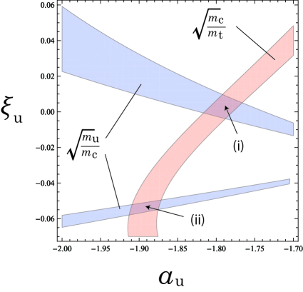
Figure 3: Allowed region in the $a_{u}$ - $\xi_{u}$ plane obtained from the up-quark mass ratios $\sqrt{m_{u}/m_{c}}$ and $\sqrt{m_{c}/m_{t}}$. The shaded areas are consistent with the observed values given in Eq.(2.13).

In model building of the down-quark sector, we give the down-quark mass ratio $m_{s}/m_{b}$ preference rather than $m_{d}/m_{s}$, because it is not so difficult to adjust the ratio $m_{d}/m_{s}$ without affecting the CKM parameter fitting as we demonstrate later. In Fig.4, we illustrate behavior of $m_{s}/m_{b}$ versus $a_{d}$. As seen in Fig.4, there are three regions which can give reasonable mass ratio $m_{s}/m_{b}$. However, the regions (ii) and (iii) cannot give reasonable CKM mixing parameters. (The region (ii) corresponds to a parameter region adopted in the old model O3PLB09 .) Hereafter, we will show the region (i) (i.e. $a_{d}\sim-17$) in detail.

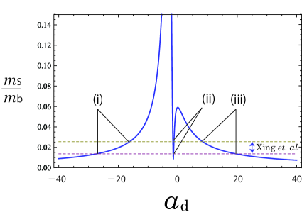
Figure 4: $a_{d}$ dependence of $m_{s}/m_{b}$. The dotted lines show the observed down-quark mass ratio $m_{s}/m_{d}=0.019+0.006$ and $0.019-0.006$.

Next, we investigate possible parameter regions which can give reasonable CKM mixing parameters. We take $|V_{us}|$, $|V_{ub}|$, $|V_{cb}|$ and $|V_{td}|$ as four independent parameters in the CKM matrix. In Fig.5, we illustrate allowed regions in the $\phi_{1}$ - $\phi_{2}$ plane obtained from $|V_{ij}|$ with $|V_{ij}|_{obs}$ under $a_{u}=-1.764$, $\xi_{u}=0.0070$ and $a_{d}=-16.6$ whose values are obtained from global best fit. As seen in Fig.5, the value of $\phi_{2}\simeq 180^{\circ}$ is in favor of the observed CKM mixing parameters. The case with $\phi_{2}=180^{\circ}$ is also illustrated in Fig.6. It is interesting that $|V_{ij}|$ take their minimum at $\phi_{1}\simeq 180^{\circ}$. From Fig.5 We find that $\phi_{1}\simeq\pm 16^{\circ}+180^{\circ}$ is in favor of the observed CKM mixing parameters.

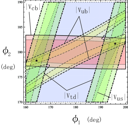
Figure 5: Allowed regions in the $\phi_{1}$ - $\phi_{2}$ plane obtained from the CKM mixing parameters $|V_{ij}|$. Shaded areas are consistent with the observed values $|V_{ij}|_{obs}$ in Eq.(2.18) . The parameter values of $a_{u}$, $\xi_{u}$ and $a_{d}$ are chosen as $a_{u}=-1.764$, $\xi_{u}=0.0070$ and $a_{d}=-16.6$ respectively. The star ($\star$) indicates the best fit points [see Eq.(3.4)].

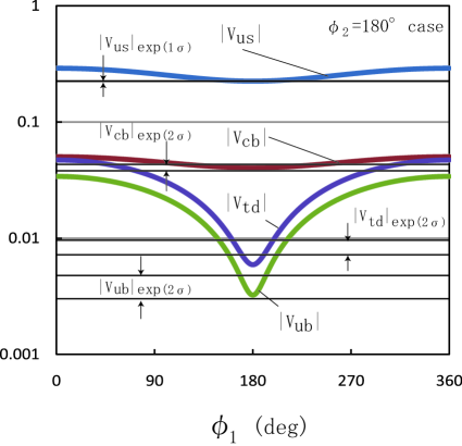
Figure 6: $\phi_{1}$ dependence of the CKM mixing parameters $|V_{ij}|$ in the case $\phi_{2}=180^{\circ}$. In the case of $\phi_{2}=180^{\circ}$, $\phi_{1}=191^{\circ}$ and $169^{\circ}$ are in favor of all the observed $|V_{ij}|_{exp}(2\sigma)$.

In conclusion, our best hit parameters are

$$a_{u}=-1.764,\ \ \ \xi_{u}=0.0070,\ \ \ a_{d}=-16.6,\ \ \ \phi_{1}=196.0^{\circ}\ (164.0^{\circ}),\ \ \ \phi_{2}=181.5^{\circ}\ (178.5^{\circ})$$

together with $\xi_{d}=0$, and then we obtain the predicted CKM mixing parameters

$$|V_{us}|=0.2259,\ \ \ |V_{cb}|=0.04141,\ \ \ |V_{ub}|=0.00418,\ \ \ |V_{td}|=0.00854.$$

However, the parameter value $a_{d}=-16.6$ gives considerably small value of $m_{d}/m_{s}$, i.e. $m_{d}/m_{s}=0.00358$. In order to correct this wrong value, we must take $m_{0d}$ with a non-zero value. By taking a value

$${m_{0d}}/m_{0}=-0.0061,$$

where $m_{0}\equiv m_{e}+m_{\mu}+m_{\tau}$, we obtain the reasonable down-quark mass ratios

$$\frac{m_{d}}{m_{s}}=0.0529,\ \ \ \ \frac{m_{s}}{m_{b}}=0.0231,$$

without affecting the CKM mixing parameters.

On the other hand, for neutrino mixing parameters, the model is essentially the same as before. In Fig.7, we illustrate $\xi_{\nu}$ dependence of the neutrino mixing parameters. As seen in Fig.7, the model can predict $\sin^{2}2\theta_{atm}\simeq 1$ and $|U_{13}|^{2}\simeq 0$ independently of $\xi_{\nu}$. The value of $\xi_{\nu}$ is determined from the observed value $\tan^{2}\theta_{solar}=0.457^{+0.038}_{-0.041}$. The value of $\xi_{\nu}$ and the neutrino mixing parameters are listed in Table I.

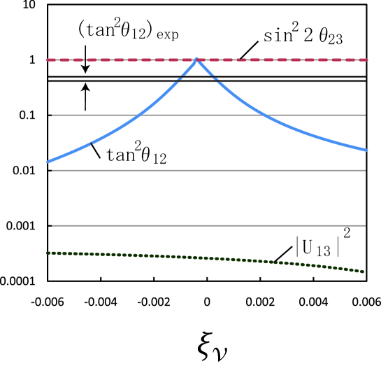
Figure 7: $\xi_{\nu}$ dependence of the neutrino mixing parameters $\tan^{2}\theta_{solar}$ (solid curve), $\sin^{2}2\theta_{atm}$ (dashed curve) and $|U_{13}|^{2}$ (dotted curve). The up-quark mass matrix parameters are chosen as $a_{u}=-1.764$ and $\xi_{u}=0.0070$.

$\xi_{\nu}$	$\tan^{2}\theta_{solar}$	$\sin^{2}2\theta_{atm}$	$|U_{13}|^{2}$
$+0.00031$	$0.457$	$0.999$	$2.56\times 10^{-4}$
$-0.00102$	$0.457$	$0.998$	$2.74\times 10^{-4}$

Table 1: Input value of $\xi_{\nu}$ and predicted values of the neutrino mixing parameters. The up-quark mass matrix parameters are chosen as $a_{u}=-1.764$ and $\xi_{u}=0.0070$ which can give reasonable up-quark mass ratios.

Let us summarize above phenomenological considerations for the mass matrices for quarks and neutrinos. By taking the phenomenological considerations $\xi_{d}=0$ and $m_{0u}=0$ into consideration, we have adopted the quark mass matrices $M_{u}^{1/2}$ and $M_{d}$ given by

$$M_{u}^{1/2}\propto M_{e}^{1/2}({\bf 1}+a_{u}X)M_{e}^{1/2}+\xi_{u}\left(M_{e}^{1/2}M_{e}^{1/2}({\bf 1}+a_{u}X)+({\bf 1}+a_{u}X)M_{e}^{1/2}M_{e}^{1/2}\right),$$

$$M_{d}\propto P_{d}\left[M_{e}^{1/2}({\bf 1}+a_{d}X)M_{e}^{1/2}+m_{0d}{\bf 1}\right]P_{d}.$$

On the other hand, the neutrino mass matrix is given by Eqs.(2.14)–(2.16). By using these mass matrices with the 7 free parameters, $a_{u}$, $\xi_{u}$, $a_{d}$, $\phi_{1}$, $\phi_{2}$, $m_{0d}$, and $\xi_{\nu}$, we have searched systematically for the parameter values which can give reasonable 4 quark mass ratios, 4 CKM quark mixing parameters, and 3 neutrino mixing parameters. (Although the values of $(m_{e},m_{\mu},m_{\tau})$ play an essential role in the present model, we have fixed those to the running mass values at $\mu=m_{Z}$, so that we do not count those as free parameters.)

IV Superpotential

In this section, by taking the phenomenological results with $\xi_{d}=0$ and $m_{0u}=0$ in the previous section into consideration, we discuss a possible form of the superpotential $W$ assuming an O(3) family symmetry. Since we consider the effective theory with $\Lambda\sim 10^{14}$ GeV, at present, it is not our chief concern whether O(3) is local or global. For the moment, we assume that O(3) is global. It should be noted that the massless states are harmless because $\Lambda$ takes an extreme large value $\Lambda\sim 10^{14}$ GeV masslessY . Under the O(3) family symmetry and conservations of U(1)_X and $R$ charges given in Table II, we obtain the following form of $W$:

$$W=W_{e}+W_{R}+W_{u}+W_{d},$$

$$W_{e}=\mu_{e}{\rm Tr}[Y_{e}\Theta_{e}]+\lambda_{e}{\rm Tr}[\Phi_{e}\Phi_{e}\Theta_{e}],$$

$$W_{R}=\mu_{R}{\rm Tr}[Y_{R}\Theta_{R}]+\frac{\lambda_{R}}{\Lambda}\left\{{\rm Tr}[(Y_{e}P_{u}\Phi_{u}+\Phi_{u}P_{u}Y_{e})\Theta_{R}]+\xi_{\nu}{\rm Tr}[(P_{u}Y_{e}\Phi_{u}+\Phi_{u}Y_{e}P_{u})\Theta_{R}]\right\},$$

$$W_{u}=\mu_{u}{\rm Tr}[Y_{u}\Theta_{u}]+\lambda_{u}{\rm Tr}[\Phi_{u}\Phi_{u}\Theta_{u}]$$

$$+\mu^{\prime}_{u}{\rm Tr}[\Phi_{u}\Theta^{\prime}_{u}]+\frac{\lambda^{\prime}_{u}}{\Lambda}\left\{{\rm Tr}[\Phi_{e}S_{u}\Phi_{e}\Theta^{\prime}_{u}]+\xi_{u}{\rm Tr}[(\Phi_{e}\Phi_{e}S_{u}+S_{u}\Phi_{e}\Phi_{e})\Theta^{\prime}_{u}]\right\},$$

$$W_{d}=\frac{\lambda_{d}}{\Lambda}{\rm Tr}[P_{d}Y_{d}P_{d}\Theta_{d}]+\frac{\lambda^{\prime}_{d}}{\Lambda}{\rm Tr}[\Phi_{e}S_{d}\Phi_{e}\Theta_{d}]+\mu_{0d}{\rm Tr}[E_{0d}\Theta_{d}],$$

where, for convenience, we have denoted linear combinations of fields $E_{q}$ and $X_{q}$ as $S_{q}=E_{q}+a_{q}X_{q}$ ($q=u,d$) and $\langle E_{q}\rangle=v_{Eq}{\bf 1}$ and $\langle X_{q}\rangle=v_{Xq}X$.

Among the SUSY vacuums which are derived from the superpotential (4.1), we take only a vacuum with $\langle\Theta_{e}\rangle=\langle\Theta_{R}\rangle=\langle\Theta_{u}\rangle=\langle\Theta^{\prime}_{u}\rangle=\langle\Theta_{d}\rangle=0$. Therefore, we can obtain VEV relations (2.6), (2.15), (3.1) and (3.2) from SUSY vacuum conditions $\partial W/\partial\Theta_{e}=0$, $\partial W/\partial\Theta_{R}=0$, $\partial W/\partial\Theta^{\prime}_{u}=0$ and $\partial W/\partial\Theta_{d}=0$, respectively. Since other conditions, for example, $\partial W/\partial Y_{e}=0$, and so on, inevitably contain a field $\Theta_{A}$ ($A=u,d,\cdots$), they cannot play effective roles in the VEV relations. (Although we did not give an explicit form of $W(\Phi_{e})$ in the present paper, we assume that $W(\Phi_{e})$ also contains $\Theta$ fields. For the form of $\langle\Phi_{e}\rangle$, Eq.(2.7), we will use the charged lepton mass values at $\mu=m_{Z}$. ) One of merits to introduce such $\Theta$ fields is that we do not need to consider contributions from higher dimensional terms with the form $({\rm Tr}[\cdots\Theta_{A}])^{n}$ ($n\geq 2$), because $\partial W/\partial\Theta_{A}$ from such a higher dimensional term always contains $\Theta_{A}$ more than one, so that such a term becomes vanishing.

Let us emphasize a role of the $R$ charges: By assuming the $R$ charge conservation with the $R$ charge assignment given in Table II, we can forbid all of higher dimensional terms with $(1/\Lambda)^{n}$ ($n\geq 2$) except for the terms given by Eqs.(4.2) - (4.5). (However, for this purpose, we must assume that our Kähler potential is given by a canonical (minimal) form.) We also note that if we assume U(1)_X only, the assignments can allow unwelcome terms in the superpotential, for example, ${\rm Tr}[S_{u}P_{u}]$, ${\rm Tr}[\Phi_{u}P_{u}\Theta_{e}]$, and so on. Such terms can be forbidden by assuming suitable $R$ charge assignments. For example, when we take $R$-charges as $R(\ell)=1-r$, $R(e^{c})=R(\nu^{c})=R(q)=R(u^{c})=R(d^{c})=1$ and $R(H_{u})=R(H_{d})=0$, we can forbid the terms ${\rm Tr}[S_{u}P_{u}]$ and ${\rm Tr}[\Phi_{u}P_{u}\Theta_{e}]$ by taking $R$ charges of other fields as given in Table II.

Fields	$Y_{e}$	$\Phi_{e}$	$\Theta_{e}$	$Y_{R}$	$\Theta_{R}$	$Y_{u}$	$\Phi_{u}$	$P_{u}$	$\Theta_{u}$	$\Theta^{\prime}_{u}$	$E_{u},X_{u}$	$Y_{d}$	$P_{d}$	$\Theta_{d}$	$E_{d},X_{d}$	$E_{0d}$
$Q_{X}$	$x_{e}$	$\frac{1}{2}x_{e}$	$-x_{e}$	$2x_{e}$	$-2x_{e}$	$x_{u}$	$\frac{1}{2}x_{u}$	$x_{e}-\frac{1}{2}x_{u}$	$-x_{u}$	$-\frac{1}{2}x_{u}$	$\frac{1}{2}x_{u}-x_{e}$	$x_{d}$	$x_{P}$	$-(x_{d}+2x_{P})$	$x_{d}+2x_{P}-x_{e}$	$x_{d}+2x_{P}$
$R$ charge	$r$	$\frac{1}{2}r$	$2-r$	$0$	$2$	$0$	$0$	$0$	$2$	$2$	$-r$	$0$	$0$	$2-r$	$0$	$r$

Table 2: U(1)_X charges of the Yukawaons. For the time being, we assign different charges for the fields $E_{u}$ and $E_{d}$ ($X_{u}$ and $X_{d}$) by assuming that those are different fields. For $R$ charges, see text.

In the phenomenological study in Sec.III, the VEV values of $\Phi_{e}$ play an essential role in evaluating the predicted values. Although it has been tried to build a model Sumino09JHEP ; e-spec_10PLB which gives VEV spectrum (2.7), it is not clear whether such a model can be applicable or not to the present model straightforwardly. In this paper, we do not give a superpotential form which can lead to the VEV spectrum (2.7). We have just assumed the VEV value given by Eq.(2.7), where we have used the values of charged lepton masses at the scale $\mu=m_{Z}$.

Also, so far, we have not given superpotential forms which lead to VEV matrices $\langle E_{q}\rangle$, $\langle X_{q}\rangle$, $\langle P_{u}\rangle$ and $\langle P_{d}\rangle$. In general, any Hermitian VEV matrix $\langle A\rangle$ can be obtained from a superpotential

$$W=\lambda_{1}({\rm Tr}[A])^{3}+\lambda_{2}{\rm Tr}[AA]{\rm Tr}[A]+\lambda_{3}{\rm Tr}[AAA].$$

[However, we must assign a U(1)_X charge $-3Q_{X}(A)$ for the coefficients $\lambda_{i}$ ($i=1,2,3$).] For example, $(\lambda_{1},\lambda_{2},\lambda_{3})=(1/6,-1/2,1/3)$ (i.e. $W={\rm det}A$) gives the form $\langle X\rangle$ given in Eq.(2.11). However, this method is not applicable to the form $\langle P_{d}\rangle$, because the VEV matrix is not Hermitian. In this paper, we have assumed these ad hoc VEV forms.

V Concluding remarks

In conclusion, we have proposed a phenomenological quark and lepton mass matrices based on a Yukawaon model. In Sec.II, we have demonstrated that the previous model O3PLB09 , in which the $CP$ violation originates only in the complex parameter $a_{d}$, cannot give reasonable CKM mixing values even if at the cost of the quark mass ratios. Differently from the previous model, in the present model, $CP$ violating phases are introduced in the phase matrix $P_{d}$ given in Eq.(3.2). In the up-quark sector, we have considered the $\xi_{u}$ term in Eq.(3.1). This comes from the fact that the terms with another order of the fields, $\Phi_{e}\Phi_{e}S_{u}+S_{u}\Phi_{e}\Phi_{e}$, cannot be, in general, forbidden compared with the order of $\Phi_{e}S_{u}\Phi_{e}$ because of the same U(1)_X charges. A similar situation have been assumed in the neutrino sector, too, i.e. the $\xi_{\nu}$ term in Eq.(4.3). (The values of $\xi_{u}$ and $\xi_{\nu}$ are very small.) In contrast to those sectors, in the down-quark sector, we have not considered such a $\xi_{d}$ term as well as an additional term $P_{d}P_{d}Y_{d}+Y_{d}P_{d}P_{d}$ corresponding to $P_{d}Y_{d}P_{d}$ in Eq.(4.5). This is a result from the phenomenological study, and the theoretical reason for the absence is unknown at present. Also we note that the phenomenological fit requires the $m_{0d}$ term added to Eq.(3.2), but it does not need an $m_{0u}$ in Eq.(3.1).

Our numerical conclusions from the present systematical study is summarized in Figs. 2-7. Especially, as seen in Fig.7, the results $\sin^{2}2\theta_{atm}\simeq 1$ and $|U_{13}|^{2}\leq 0.005$ are insensitive to the value of the parameter $\xi_{\nu}$. In other words, if $|U_{13}|^{2}\sim 0.01$ (the possibility was pointed out by Fogli, et al. Fogli ) is established experimentally, the present model will be ruled out, or it will need a drastic revision.

We have been able to obtain reasonable parameter fitting not only for the observed lepton mixing but also for the observed quark mixing. However, the model still includes ad hoc assumptions. We consider that it is important to clarify what parts are problems to get a good fitting of the data for the next step of the investigation. Our model building will proceed step by step.

Acknowledgments

The authors would like to thank T. Yamashita for his valuable and helpful comments, especially on the effective theory. One of authors (Y.K.) is supported by the Grant-in-Aid for Scientific Research (C), JSPS, No.21540266.

References

• (1) D. G. Michael et al., MINOS collaboration, Phys. Rev. Lett. 97, 191801 (2006); J. Hosaka, et al., Super-Kamiokande collaboration, Phys. Rev. D 74, 032002 (2006).
• (2) B. Aharmim, et al., SNO collaboration, Phys. Rev. Lett. 101, 111301 (2008). Also, see S. Abe, et al., KamLAND collaboration, Phys. Rev. Lett. 100, 221803 (2008).
• (3) P. F. Harrison, D. H. Perkins and W. G. Scott, Phys. Lett. B 458, 79 (1999); Phys. Lett. B 530, 167 (2002); Z.-z. Xing, Phys. Lett. B 533, 85 (2002); P. F. Harrison and W. G. Scott, Phys. Lett. B 535, 163 (2002); Phys. Lett. B 557, 76 (2003); E. Ma, Phys. Rev. Lett. 90, 221802 (2003); C. I. Low and R. R. Volkas, Phys. Rev. D 68, 033007 (2003).
• (4) Y. Koide, Phys. Lett. B 665, 227 (2008).
• (5) Y. Koide, Phys. Lett. B 680, 76 (2009).
• (6) Y. Koide, Phys. Rev. D 78, 037302 (2008).
• (7) Y. Sumino, Phys. Lett. B 671, 477 (2009).
• (8) Y. Sumino, JHEP 0905, 075 (2009).
• (9) Y. Koide, Phys. Lett. B 687, 219 (2010).
• (10) Y. Koide and H. Fusaoka, Z. Phys. C 71, 459 (1996); Prog. Theor. Phys. 97, 459 (1997).
• (11) Z.-z. Xing, H. Zhang and S. Zhou, Phys. Rev. D 77, 113016 (2008). And also see, H. Fusaoka and Y. Koide, Phys. Rev. D 57, 3986 (1998).
• (12) Particle Data Group, K. Nakamura, et al., J. Phys. G 37, 075021 (2010).
• (13) Y. Koide, IJMPA 25, 1725 (2010).
• (14) G. L. Fogli, et al., Phys. Rev. Lett. 101, 14181 (2008).