Uniqueness of collinear solutions for the relativistic three-body problem

Abstract

Continuing work initiated in an earlier publication [Yamada, Asada, Phys. Rev. D 82, 104019 (2010)], we investigate collinear solutions to the general relativistic three-body problem. We prove the uniqueness of the configuration for given system parameters (the masses and the end-to-end length). First, we show that the equation determining the distance ratio among the three masses, which has been obtained as a seventh-order polynomial in the previous paper, has at most three positive roots, which apparently provide three cases of the distance ratio. It is found, however, that, even for such cases, there exists one physically reasonable root and only one, because the remaining two positive roots do not satisfy the slow motion assumption in the post-Newtonian approximation and are thus discarded. This means that, especially for the restricted three-body problem, exactly three positions of a third body are true even at the post-Newtonian order. They are relativistic counterparts of the Newtonian Lagrange points $L_{1}$, $L_{2}$ and $L_{3}$. We show also that, for the same masses and full length, the angular velocity of the post-Newtonian collinear configuration is smaller than that for the Newtonian case. Provided that the masses and angular rate are fixed, the relativistic end-to-end length is shorter than the Newtonian one.

I Introduction

The three-body problem in Newtonian gravity belongs among classical problems in astronomy and physics (e.g, Danby ; Goldstein ). In 1765, Euler found a collinear solution for the restricted three-body problem, where one of three bodies is a test mass. Soon after, his solution was extended for a general three-body problem by Lagrange, who also found an equilateral triangle solution in 1772. Now, the solutions for the restricted three-body problem are called Lagrange points $L_{1},L_{2},L_{3},L_{4}$ and $L_{5}$, which are described in textbooks of classical mechanics Goldstein . SOHO (Solar and Heliospheric Observatory) and WMAP (Wilkinson Microwave Anisotropy Probe) launched by NASA are in operation at the Sun-Earth $L_{1}$ and $L_{2}$, respectively. LISA (Laser Interferometer Space Antenna) pathfinder is planned to go to $L_{1}$. Lagrange points have recently attracted renewed interests for relativistic astrophysics THA ; Asada ; SM ; Schnittman , where they have discussed the gravitational radiation reaction on $L_{4}$ and $L_{5}$ analytically Asada and by numerical methods THA ; SM ; Schnittman .

As a pioneering work, Nordtvedt pointed out that the location of the triangular points is very sensitive to the ratio of the gravitational mass to the inertial one Nordtvedt . Along this course, it is interesting as a gravity experiment to discuss the three-body coupling terms at the post-Newtonian order, because some of the terms are proportional to a product of three masses as $M_{1}\times M_{2}\times M_{3}$. Such a term appears only for relativistic three (or more) body systems: For a relativistic binary with two masses $M_{1}$ and $M_{2}$, there exist $M_{1}^{2}M_{2}$ and $M_{1}M_{2}^{2}$ without such a three-mass product. For a Newtonian three-body system, we have only the two-body coupling terms proportional to $M_{1}M_{2}$, $M_{2}M_{3}$ or $M_{3}M_{1}$.

The relativistic perihelion advance of Mercury is detected only after much larger shifts due to Newtonian perturbations by other planets such as the Venus and Jupiter are taken into account in the astrometric data analysis. In this sense, effects by the three body coupling are worthy to investigate. Nevertheless, most of post-Newtonian works have focused on either compact binaries because of our interest in gravitational waves astronomy or N-body equation of motion (and coordinate systems) in the weak field such as the solar system (e.g. Brumberg ). Actually, future space astrometric missions such as Gaia GAIA ; JASMINE require a general relativistic modeling of the solar system within the accuracy of a micro arc-second Klioner . Furthermore, a binary plus a third body have been discussed also for perturbations of gravitational waves induced by the third body ICTN ; Wardell ; CDHL ; GMH .

After efforts to find a general solution, Poincare proved that it is impossible to describe all the solutions to the three-body problem even for the $1/r$ potential. Namely, we cannot analytically obtain all the solutions. Nevertheless, the number of new solutions is increasing Marchal . Therefore, the three-body problem still remains an open issue even for Newton gravity.

The theory of general relativity is currently the most successful gravitational theory describing the nature of space and time. Hence, it is important to take account of general relativistic effects on three-body configurations. The figure-eight configuration that was found decades ago Moore ; CM has been recently studied at the first post-Newtonian ICA and also the second post-Newtonian orders LN . According to their numerical investigations, the solution remains true with a slight change in the figure-eight shape because of relativistic effects.

On the other hand, the post-Newtonian collinear configuration obtained in the previous paper YA may offer a useful toy model for relativistic three-body interactions, because it is tractable by hand without numerical simulations. This solution is a relativistic extension of Euler’s collinear one, where three bodies move around the common center of mass with the same orbital period and always line up.

In fact, their formulation leads to a seventh-order equation determining the distance ratio among masses YA . Here, it should be noted that only positive roots are acceptable, because the distance ratio must be positive. Properties of the master equation have not been known yet. How many positive roots for it are there? The main purpose of this paper is to analytically investigate the number of the positive roots. In particular, we shall prove the uniqueness of the configuration for given system parameters (the masses and the end-to-end length).

This paper is organized as follows. In section II, we briefly summarize formulations for collinear solutions at the Newtonian and post-Newtonian orders. We discuss positive roots for the seventh-order equation for determining the distance ratio in section III. In section IV, we show the uniqueness of the configuration for given system parameters (the masses and the end-to-end length). We also compare the angular velocity of the post-Newtonian collinear configuration with that for the Newtonian one. Section V is devoted to the conclusion. We provide some detailed calculations regarding the angular velocity of collinear configurations in the Appendix.

Throughout this paper, we take the units of $G=c=1$.

II Equation for the distance ratio among three masses

Let us begin by summarizing the derivation of the Euler’s collinear solution for the circular three-body problem in Newton gravity. We consider Euler’s solution, for which each mass moves around their common center of mass denoted as $\mbox{\boldmath$X$}_{G}$ with a constant angular velocity $\omega$. Hence, it is convenient to use the corotating frame with the same angular velocity $\omega$. We choose an orbital plane normal to the total angular momentum as the $x-y$ plane in such a corotating frame. We locate all the three bodies on a single line, along which we take the $x$-coordinate. The location of each mass $M_{I}$ $(I=1,2,3)$ is written as $\mbox{\boldmath$X$}_{I}\equiv(x_{I},0)$. Without loss of generality, we assume $x_{3}<x_{2}<x_{1}$. Let $R_{I}$ define the relative position of each mass with respective to the center of mass $\mbox{\boldmath$X$}_{G}\equiv(x_{G},0)$, namely $R_{I}\equiv x_{I}-x_{G}$ ($R_{I}\neq|\mbox{\boldmath$X$}_{I}|$ unless $x_{G}=0$). We choose $x=0$ between $M_{1}$ and $M_{3}$. We thus have $R_{3}<R_{2}<R_{1}$, $R_{3}<0$ and $R_{1}>0$.

It is convenient to define a ratio as $R_{23}/R_{12}=z$, which is an important variable in the following formulation. Then we have $R_{13}=(1+z)R_{12}$. The equation of motion becomes

$$R_{1}\omega^{2} = \frac{M_{2}}{R_{12}^{2}}+\frac{M_{3}}{R_{13}^{2}},$$ (1)

$$R_{2}\omega^{2} = -\frac{M_{1}}{R_{12}^{2}}+\frac{M_{3}}{R_{23}^{2}},$$ (2)

$$R_{3}\omega^{2} = -\frac{M_{1}}{R_{13}^{2}}-\frac{M_{2}}{R_{23}^{2}},$$ (3)

where we define

$$\mbox{\boldmath$R$}_{IJ} \equiv \mbox{\boldmath$X$}_{I}-\mbox{\boldmath$X$}_{J},$$ (4)

$$R_{IJ} \equiv |\mbox{\boldmath$R$}_{IJ}|.$$ (5)

First, we subtract Eq. (2) from Eq. (1) and Eq. (3) from Eq. (2) and use $R_{12}\equiv|\mbox{\boldmath$X$}_{1}-\mbox{\boldmath$X$}_{2}|$ and $R_{23}\equiv|\mbox{\boldmath$X$}_{2}-\mbox{\boldmath$X$}_{3}|$. Such a subtraction procedure will be useful also at the post-Newtonian order, because we can avoid directly using the post-Newtonian center of mass MTW ; LL . Next, we compute a ratio between them to delete $\omega^{2}$. Hence a fifth-order equation is obtained as

$$(M_{1}+M_{2})z^{5}+(3M_{1}+2M_{2})z^{4}+(3M_{1}+M_{2})z^{3}-(M_{2}+3M_{3})z^{2}-(2M_{2}+3M_{3})z-(M_{2}+M_{3})=0.$$ (6)

Now we have a condition as $z>0$. Descartes’ rule of signs (e.g., Waerden ) states that the number of positive roots either equals that of sign changes in coefficients of a polynomial or less than it by a multiple of two. According to this rule, Eq. (6) has only the positive root $z>0$, though such a fifth-order equation cannot be solved in algebraic manners as shown by Galois (e.g., Waerden ). After obtaining $z$, one can substitute it into a difference, for instance between Eqs. (1) and (3). Hence we get $\omega$.

In order to include the dominant part of general relativistic effects, we take account of the terms at the first post-Newtonian order. Namely, the massive bodies obey the Einstein-Infeld-Hoffman (EIH) equation of motion as MTW ; LL

$$\frac{d\mbox{\boldmath$v$}_{K}}{dt} = \sum_{A\neq K}\mbox{\boldmath$R$}_{AK}\frac{M_{A}}{R_{AK}^{3}}\left[1-4\sum_{B\neq K}\frac{M_{B}}{R_{BK}}-\sum_{C\neq A}\frac{M_{C}}{R_{CA}}\left(1-\frac{\mbox{\boldmath$R$}_{AK}\cdot\mbox{\boldmath$R$}_{CA}}{2R_{CA}^{2}}\right)\right.$$ (7)

$$\left.~{}~{}~{}~{}~{}~{}~{}~{}~{}~{}~{}~{}~{}~{}~{}~{}~{}~{}~{}~{}~{}+v_{K}^{2}+2v_{A}^{2}-4\mbox{\boldmath$v$}_{A}\cdot\mbox{\boldmath$v$}_{K}-\frac{3}{2}\left(\mbox{\boldmath$v$}_{A}\cdot\mbox{\boldmath$n$}_{AK}\right)^{2}\right]$$

$$-\sum_{A\neq K}(\mbox{\boldmath$v$}_{A}-\mbox{\boldmath$v$}_{K})\frac{M_{A}\mbox{\boldmath$n$}_{AK}\cdot(3\mbox{\boldmath$v$}_{A}-4\mbox{\boldmath$v$}_{K})}{R_{AK}^{2}}$$

$$+\frac{7}{2}\sum_{A\neq K}\sum_{C\neq A}\mbox{\boldmath$R$}_{CA}\frac{M_{A}M_{C}}{R_{AK}R_{CA}^{3}},$$

where $\mbox{\boldmath$v$}_{I}$ denotes the velocity of each mass in an inertial frame and we define

$$\mbox{\boldmath$n$}_{IJ} \equiv \frac{\mbox{\boldmath$R$}_{IJ}}{R_{IJ}},$$ (8)

and we assume the slow motion ($|\mbox{\boldmath$v$}_{I}|\ll c$).

We obtain a lengthy form of the equation of motion for each body. By subtracting the post-Newtonian equation of motion for $M_{3}$ from that for $M_{1}$ for instance, we obtain the equation as YA

$$R_{13}\omega^{2}=F_{N}+F_{M}+F_{V}\omega^{2},$$ (9)

where we denote $a\equiv R_{13}$ and the Newtonian term $F_{N}$ and the post-Newtonian parts $F_{M}$ (dependent on the masses only) and $F_{V}$ (velocity-dependent part divided by $\omega^{2}$) are defined as

$$F_{N} = \frac{M}{a^{2}z^{2}}\Biggl{[}(\nu_{1}+\nu_{3})z^{2}+(1-\nu_{1}-\nu_{3})(1+z^{2})(1+z)^{2}\Biggr{]},$$ (10)

$$F_{M} = -\frac{M^{2}}{a^{3}z^{3}}\Biggl{[}(4-4\nu_{1}+\nu_{3})(1-\nu_{1}-\nu_{3})$$ (11)

$$\mspace{65.0mu}+(12-7\nu_{1}+3\nu_{3})(1-\nu_{1}-\nu_{3})z$$

$$\mspace{65.0mu}+(12-\nu_{1}+\nu_{3})(1-\nu_{1}-\nu_{3})z^{2}$$

$$\mspace{65.0mu}+(8-7\nu_{1}-7\nu_{3}+8\nu_{1}\nu_{3}+3\nu_{1}^{2}+3\nu_{3}^{2})z^{3}$$

$$\mspace{65.0mu}+(12+\nu_{1}-\nu_{3})(1-\nu_{1}-\nu_{3})z^{4}$$

$$\mspace{65.0mu}+(12+3\nu_{1}-7\nu_{3})(1-\nu_{1}-\nu_{3})z^{5}$$

$$\mspace{65.0mu}+(4+\nu_{1}-4\nu_{3})(1-\nu_{1}-\nu_{3})z^{6}\Biggr{]},$$

$$F_{V} = \frac{M}{(1+z)^{2}z^{2}}\Biggl{[}-\nu_{1}^{2}(1-\nu_{1}-\nu_{3})$$ (12)

$$\mspace{91.0mu}-2\nu_{1}(1+\nu_{1}-\nu_{3})(1-\nu_{1}-\nu_{3})z$$

$$\mspace{91.0mu}+(2-2\nu_{1}+\nu_{3}+6\nu_{1}\nu_{3}-3\nu_{3}^{2}+\nu_{1}^{3}-3\nu_{1}^{2}\nu_{3}-3\nu_{1}\nu_{3}^{2}+\nu_{3}^{3})z^{2}$$

$$\mspace{91.0mu}+2(2-\nu_{1}-\nu_{3})(1+\nu_{1}+\nu_{3}-\nu_{1}^{2}+\nu_{1}\nu_{3}-\nu_{3}^{2})z^{3}$$

$$\mspace{91.0mu}+(2+\nu_{1}-2\nu_{3}-3\nu_{1}^{2}+6\nu_{1}\nu_{3}+\nu_{1}^{3}-3\nu_{1}^{2}\nu_{3}-3\nu_{1}\nu_{3}^{2}+\nu_{3}^{3})z^{4}$$

$$\mspace{91.0mu}-2\nu_{3}(1-\nu_{1}+\nu_{3})(1-\nu_{1}-\nu_{3})z^{5}$$

$$\mspace{91.0mu}-\nu_{3}^{2}(1-\nu_{1}-\nu_{3})z^{6}\Biggr{]},$$

respectively. Here, we define the mass ratio as $\nu_{I}\equiv M_{I}/M$ for the total mass $M\equiv\sum_{I}M_{I}$ and make a frequent use of $\nu_{2}=1-\nu_{1}-\nu_{3}$. It should be noted that in this truncated calculation we ignore the second post-Newtonian (or higher order) contributions so that we can replace, for instance, $v_{1}$ by $R_{1}\omega$ (using the Newtonian $R_{1}$) in post-Newtonian velocity-dependent terms such as $v_{1}^{2}$.

In a similar manner to the above Newtonian formulation, straightforward but lengthy calculations lead to a seventh-order equation as YA

$$F(z)\equiv\sum_{k=0}^{7}A_{k}z^{k}=0,$$ (13)

where we define

$$A_{7} = \frac{M}{a}\Biggl{[}-4-2(\nu_{1}-4\nu_{3})+2(\nu_{1}^{2}+2\nu_{1}\nu_{3}-2\nu_{3}^{2})-2\nu_{1}\nu_{3}(\nu_{1}+\nu_{3})\Biggr{]},$$ (14)

$$A_{6} = 1-\nu_{3}+\frac{M}{a}\Biggl{[}-13-(10\nu_{1}-17\nu_{3})+2(2\nu_{1}^{2}+8\nu_{1}\nu_{3}-\nu_{3}^{2})$$ (15)

$$\mspace{103.0mu}+2(\nu_{1}^{3}-2\nu_{1}^{2}\nu_{3}-3\nu_{1}\nu_{3}^{2}-\nu_{3}^{3})\Biggr{]},$$

$$A_{5} = 2+\nu_{1}-2\nu_{3}+\frac{M}{a}\Biggl{[}-15-(18\nu_{1}-5\nu_{3})+4(5\nu_{1}\nu_{3}+4\nu_{3}^{2})$$ (16)

$$\mspace{148.0mu}+6(\nu_{1}^{3}-\nu_{1}\nu_{3}^{2}-\nu_{3}^{3})\Biggr{]},$$

$$A_{4} = 1+2\nu_{1}-\nu_{3}+\frac{M}{a}\Biggl{[}-6-2(5\nu_{1}+2\nu_{3})-4(2\nu_{1}^{2}-\nu_{1}\nu_{3}-4\nu_{3}^{2})$$ (17)

$$\mspace{148.0mu}+2(3\nu_{1}^{3}+\nu_{1}^{2}\nu_{3}-2\nu_{1}\nu_{3}^{2}-3\nu_{3}^{3})\Biggr{]},$$

$$A_{3} = -(1-\nu_{1}+2\nu_{3})+\frac{M}{a}\Biggl{[}6+2(2\nu_{1}+5\nu_{3})-4(4\nu_{1}^{2}+\nu_{1}\nu_{3}-2\nu_{3}^{2})$$ (18)

$$\mspace{177.0mu}+2(3\nu_{1}^{3}+2\nu_{1}^{2}\nu_{3}-\nu_{1}\nu_{3}^{2}-3\nu_{3}^{3})\Biggr{]},$$

$$A_{2} = -(2-2\nu_{1}+\nu_{3})+\frac{M}{a}\Biggl{[}15-(5\nu_{1}-18\nu_{3})-4(4\nu_{1}^{2}+5\nu_{1}\nu_{3})$$ (19)

$$\mspace{177.0mu}+6(\nu_{1}^{3}+\nu_{1}^{2}\nu_{3}-\nu_{3}^{3})\Biggr{]},$$

$$A_{1} = -(1-\nu_{1})+\frac{M}{a}\Biggl{[}13-(17\nu_{1}-10\nu_{3})+2(\nu_{1}^{2}-8\nu_{1}\nu_{3}-2\nu_{3}^{2})$$ (20)

$$\mspace{130.0mu}+2(\nu_{1}^{3}+3\nu_{1}^{2}\nu_{3}+2\nu_{1}\nu_{3}^{2}-\nu_{3}^{3})\Biggr{]},$$

$$A_{0} = \frac{M}{a}\Biggl{[}4-2(4\nu_{1}-\nu_{3})+2(2\nu_{1}^{2}-2\nu_{1}\nu_{3}-\nu_{3}^{2})+2\nu_{1}\nu_{3}(\nu_{1}+\nu_{3})\Biggr{]}.$$ (21)

Here, the sign of Eq. (21) is chosen so that it can agree with the fifth-order equation Eq. (6) in the Newtonian limit of $M/a\to 0$. This seventh-order equation is antisymmetric for exchanges between $\nu_{1}$ and $\nu_{3}$, only if one makes a change as $z\to 1/z$. This antisymmetry may validate the complicated form of each coefficient.

Once a positive root for Eq. (13) is found, the root $z$ can be substituted into Eq. (9) in order to obtain the angular velocity $\omega$.

The angular velocity including the post-Newtonian effects is obtained from Eq. (9) as YA

$$\omega=\omega_{N}\left(1+\frac{F_{M}}{2F_{N}}+\frac{F_{V}}{2R_{13}}\right),$$ (22)

where $\omega_{N}\equiv(F_{N}/R_{13})^{1/2}$ denotes the angular velocity of the Newtonian collinear orbit. Note that the slow motion is assumed to derive Eq. (22) which is analogous to Kepler’s third law.

III Existence of positive roots

In this section, we show that there always exist positive roots for the seventh-order equation that has been derived as Eq. (13). This is nothing but the existence of the post-Newtonian collinear solution.

For later convenience, we recover $\nu_{2}$ and thus rewrite a coefficient $A_{0}$ as

$$A_{0}=2\frac{M}{a}(\nu_{2}+\nu_{3})(2\nu_{2}+2\nu_{3}+\nu_{2}\nu_{3}),$$ (23)

which immediately leads to $A_{0}>0$.

In a similar manner, one can show $A_{7}<0$. An alternative but powerful way to see this is using the antisymmetry of the seventh-order equation for transformations between masses $M_{1}$ and $M_{3}$ as $\nu_{1}\leftrightarrow\nu_{3}$ and $z\leftrightarrow 1/z$. This transformation makes a change as $A_{0}\to-A_{7}$. By using $A_{0}>0$, therefore, we have always $A_{7}<0$.

Bringing the above results together, we have $F(0)=A_{0}>0$ and $F(\infty)=A_{7}z^{7}|_{z\to\infty}<0$. Therefore, the number of positive roots for $F(z)=0$ either equals to one or more than it by a multiple of two.

Let us investigate the seventh-order equation in order to more precisely determine the number of positive roots. We decompose each coefficient $A_{k}$ into the Newtonian part $A_{Nk}$ and the post-Newtonian one $A_{PNk}$. Note that $A_{Nk}$ agrees with the coefficient of $z^{k-1}$ (but not $z^{k}$) in Eq. (6). In the Newtonian fifth-order equation by Eq. (6), we have $A_{N6}>0$, $A_{N5}>0$, $A_{N4}>0$, $A_{N3}<0$, $A_{N2}<0$, $A_{N1}<0$. In the post-Newtonian approximation, the post-Newtonian parts must be much smaller than the Newtonian ones ($|A_{PNk}|\ll|A_{Nk}|$ for each $k$), so that the post-Newtonian correction cannot change the sign of each coefficient $A_{k}$. We thus have $A_{6}>0$, $A_{5}>0$, $A_{4}>0$, $A_{3}<0$, $A_{2}<0$, $A_{1}<0$. By combining them with $A_{7}<0$ and $A_{0}>0$, the number of sign changes of the coefficients in Eq. (13) is necessarily three. Therefore, Descartes’ rule of signs indicates that Eq. (13) has either one or three roots. We can easily understand that one of them is a correction to the Newtonian orbit. What are the other two roots? We shall investigate them in next section.

IV Uniqueness of the post-Newtonian collinear solution

Figure 1 shows that the equation has three positive roots, where we assume $\nu_{1}=1/7$, $\nu_{2}=5/7$, $\nu_{3}=1/7$, $a/M=10^{4}$ ($v\sim 10^{-2}$). Table 1 shows numerical values of $z$, $\omega$ and $a\omega$ for Figure 1. Two out of the three roots do not satisfy a slow-motion condition for the post-Newtonian approximation as shown below.

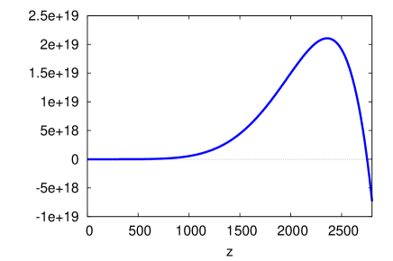
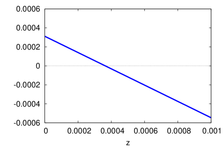
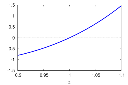
Figure 1: Top panel: The seventh-order polynomial in the L.H.S. of Eq. (13). The horizontal axis is chosen as $z$. We take $\nu_{1}=1/7$, $\nu_{2}=5/7$, $\nu_{3}=1/7$, $a/M=10^{4}$ ($v\sim 10^{-2}$) in order to exaggerate small effects in these figures. Clearly such a symmetric choice of the mass ratios produces a trivial root as $z=1$, which makes it easy to check numerical calculations. $M_{2}$ is relatively large so that the centrifugal force can be large.
Middle panel: The seventh-order polynomial around the smallest positive root $z_{S}$.
Bottom panel: The polynomial around the moderate positive root.

Table 1: Values of $z$, $\omega$ and $a\omega$ for Figure 1. Here are three positive roots, where we assume $z_{1}<z_{2}<z_{3}$.

	$z_{1}$	$z_{2}$	$z_{3}$
z	3.635$\times 10^{-4}$	1.000	2751
$\omega$	8.723$\times 10^{-5}$	2.449$\times 10^{-6}$	8.723$\times 10^{-5}$
$a\omega$	0.8723	0.02449	0.8723

Here we show that the remaining two positive roots must be discarded. Because of the antisymmetry of Eq. (13) for the transformation as $z\leftrightarrow 1/z$, the two roots must be a pair through this transformation associated with exchanges between $M_{1}$ and $M_{3}$. Let the smaller root and the larger one be denoted as $z_{S}$ and $z_{L}$, respectively.

First, we consider the smallest positive root $z_{S}$, where we assume $z_{S}\ll 1$. Then, Eq.(13) is approximated as

$$A_{1}z_{S}+A_{0}=0,$$ (24)

where $A_{0}$ starts at the post-Newtonian order without Newtonian terms and $A_{1}=A_{N1}+A_{PN1}$ has both the Newtonian terms and post-Newtonian corrections ($|A_{N1}|\gg|A_{PN1}|$). We thus obtain an approximate form of the smallest root as

$$z_{S} = -\frac{A_{0}}{A_{N1}}$$ (25)

$$= O\left(\frac{M}{a}\right),$$

where we used Eqs. (20) and (21). This implies that $z_{S}$ is indeed of the post-Newtonian order, in consistent with $z_{S}\ll 1$. At this point, however, we cannot discard this smallest root $z_{S}$.

As a next step, let us make an order-of-magnitude estimation for the angular velocity $\omega_{S}$ that satisfies Eq. (9) for $z_{S}$, where $\omega_{S}$ denotes the angular velocity corresponding to $z_{S}$. We obtain from Eqs. (10), (11) and (12)

$$F_{N} = O\left(\frac{M}{a^{2}z_{S}^{2}}\right)$$ (26)

$$= O\left(\frac{1}{M}\right),$$

$$F_{M} = O\left(\frac{M^{2}}{a^{3}z_{S}^{3}}\right)$$ (27)

$$= O\left(\frac{1}{M}\right),$$

$$F_{V} = O\left(\frac{M}{z_{S}^{2}}\right)$$ (28)

$$= O\left(\frac{a^{2}}{M}\right).$$

We thus find $R_{13}=a\ll F_{V}$ because $M\ll a$. Therefore, we find $F_{N}\sim F_{M}\sim F_{V}\omega_{S}^{2}\gg R_{13}\omega_{S}^{2}$ in Eq. (9). This leads to

$$\omega_{S} = O\left(\frac{1}{a}\right),$$ (29)

though $\omega_{N}^{2}=O(M/a^{3})$ for the Newtonian case. Eq. (29) implies an extremely fast rotation, since the rotational velocity becomes $v_{S}\approx a\omega_{S}=O(1)$, namely, comparable to the speed of light. This unacceptable branch of such an extremely fast motion contradicts the post-Newtonian approximation and does not satisfy Eq. (22). Hence, $z_{S}$ must be abandoned.

Next, we consider the largest positive root $z_{L}$, where we assume $z_{L}\gg 1$. Then, Eq.(13) is approximated as

$$A_{7}z_{L}+A_{6}=0,$$ (30)

where $A_{7}$ starts at the post-Newtonian order without Newtonian terms and $A_{6}=A_{N6}+A_{PN6}$ has both the Newtonian terms and post-Newtonian corrections ($|A_{N6}|\gg|A_{PN6}|$). We thus obtain an approximate form of the largest root as

$$z_{L} = -\frac{A_{7}}{A_{N6}}$$ (31)

$$= O\left(\frac{a}{M}\right),$$

where we used Eqs. (14) and (15). This implies that $z_{L}^{-1}$ is indeed of the post-Newtonian order, in consistent with $z_{L}\gg 1$. At this point, however, we cannot discard this largest root $z_{L}$.

As a next step, let us make an order-of-magnitude estimation for the angular velocity $\omega_{L}$ that satisfies Eq. (9) for $z_{L}$, where $\omega_{L}$ denotes the angular velocity corresponding to $z_{L}$. We obtain from Eqs. (10), (11) and (12)

$$F_{N} = O\left(\frac{Mz_{L}^{2}}{a^{2}}\right)$$ (32)

$$= O\left(\frac{1}{M}\right),$$

$$F_{M} = O\left(\frac{M^{2}z_{L}^{3}}{a^{3}}\right)$$ (33)

$$= O\left(\frac{1}{M}\right),$$

$$F_{V} = O\left(Mz_{L}^{2}\right)$$ (34)

$$= O\left(\frac{a^{2}}{M}\right).$$

We thus find $R_{13}=a\ll F_{V}$ because $M\ll a$. Therefore, we find $F_{N}\sim F_{M}\sim F_{V}\omega_{L}^{2}\gg R_{13}\omega_{L}^{2}$ in Eq. (9). This leads to

$$\omega_{L} = O\left(\frac{1}{a}\right),$$ (35)

though $\omega_{N}^{2}=O(M/a^{3})$ for the Newtonian case. Eq. (35) implies an extremely fast rotation, since the rotational velocity becomes $v_{L}\approx a\omega_{L}=O(1)$, namely, comparable to the speed of light. This unacceptable branch of such an extremely fast motion contradicts the post-Newtonian approximation and does not satisfy Eq. (22). Hence, also $z_{L}$ must be abandoned.

We should remember the transformation as $z\leftrightarrow 1/z$, namely $1\leftrightarrow 3$. Hence, $z_{S}$ and $z_{L}$ correspond to each other as $z_{S}=1/z_{L}$. In this sense, it seems natural that the above argument for discarding $z_{L}$ is very similar to that of $z_{S}$.

As a result, two of the three positive roots are discarded as unphysical ones. Hence, we complete the proof of the uniqueness.

We mention an application of the uniqueness theorem for the restricted three-body problem. We have three possibilities for choosing a test mass as $M_{1}=0$, $M_{2}=0$ or $M_{3}=0$. For each case, we have only the single collinear solution. Therefore, the three equilibrium points exist along the symmetry axis of the system, and they are a generalization of Lagrange points $L_{1}$, $L_{2}$ and $L_{3}$.

Before closing this section, we mention an interesting property of the angular velocity of the collinear configurations. For the same masses and full length, we have always an inequality as

$$\omega<\omega_{N},$$ (36)

which means that the post-Newtonian orbital period measured in the coordinate time is longer than the Newtonian one. Provided that the masses and angular rate are fixed, the relativistic length $a$ is shorter than the Newtonian one. Detailed calculations are given in the Appendix.

V Conclusion

We proved the uniqueness of the collinear configuration for given system parameters (the masses and the end-to-end length). It was shown that the equation determining the distance ratio among the three masses, which has been obtained as a seventh-order polynomial in the previous paper, has at most three positive roots, which apparently provide three cases of the distance ratio. It was found, however, that there exists one physically acceptable root and only one. The remaining two positive roots are discarded in the sense that they do not satisfy the slow motion ansatz in the post-Newtonian approximation.

Especially for the restricted three-body problem, exactly three positions of a third body are true even at the post-Newtonian order. They are relativistic counterparts of the Newtonian Lagrange points $L_{1}$, $L_{2}$ and $L_{3}$.

It was shown also that, for the same masses and full length, the angular velocity of the post-Newtonian collinear configuration is smaller than that for the Newtonian case. Provided that the masses and angular rate are fixed, the relativistic length $a$ is shorter than the Newtonian one.

Our way of discussion seems to work at the second (and higher) post-Newtonian orders, because the slow motion approximation is a key in the above proof. Therefore, the uniqueness of collinear configurations for a three-body system may be true even at higher orders, precisely speaking, if the configuration has the Newtonian limit. It is an open question whether fully general relativistic systems admit a particular solution that can appear only for a fast motion case and thus has no Newtonian limit.

We would like to thank the referee for useful comments on the earlier version of the manuscript. We are grateful to Y. Kojima for useful conversations. This work was supported in part (H.A.) by a Japanese Grant-in-Aid for Scientific Research from the Ministry of Education, No. 21540252.

Appendix A Detailed calculations on the angular velocity

Let us prove $\omega<\omega_{N}$. Eq. (22) is rewritten as

$$\frac{\omega-\omega_{N}}{\omega_{N}}=\frac{F_{M}R_{13}+F_{V}F_{N}}{2F_{N}R_{13}}.$$ (37)

Here, $F_{N}$ is positive and thus the denominator of the R.H.S. of Eq. (37) is always positive. What we have to do is to investigate the sign of the numerator for the R.H.S. of Eq. (37). The numerator is factored as

$$\frac{M^{2}}{a^{2}z^{4}(1+z)^{2}}\times\sum_{k=0}^{10}a_{k}z^{k},$$ (38)

where we define

$$a_{10} = -(1-\nu_{1}-\nu_{3})^{2}\nu_{3}^{2},$$ (39)

$$a_{9} = -(1-\nu_{1}-\nu_{3})(4+\nu_{1}-2\nu_{3}-4\nu_{1}\nu_{3}+2\nu_{3}^{2}+2\nu_{1}^{2}\nu_{3}-2\nu_{1}\nu_{3}^{2}-4\nu_{3}^{3}),$$ (40)

$$a_{8} = -(1-\nu_{1}-\nu_{3})(18+4\nu_{1}-9\nu_{3}+3\nu_{1}^{2}-14\nu_{1}\nu_{3}$$ (41)

$$\mspace{120.0mu}+2\nu_{3}^{2}-\nu_{1}^{3}+7\nu_{1}^{2}\nu_{3}+2\nu_{1}\nu_{3}^{2}-6\nu_{3}^{3}),$$

$$a_{7} = -(1-\nu_{1}-\nu_{3})(32+4\nu_{1}-13\nu_{3}+12\nu_{1}^{2}-18\nu_{1}\nu_{3}$$ (42)

$$\mspace{120.0mu}+10\nu_{3}^{2}-4\nu_{1}^{3}+8\nu_{1}^{2}\nu_{3}+4\nu_{1}\nu_{3}^{2}-8\nu_{3}^{3}),$$

$$a_{6} = -(30-30\nu_{1}-37\nu_{3}+19\nu_{1}^{2}-12\nu_{1}\nu_{3}+27\nu_{3}^{2}-22\nu_{1}^{3}+18\nu_{1}^{2}\nu_{3}$$ (43)

$$\mspace{20.0mu}+12\nu_{1}\nu_{3}^{2}-28\nu_{3}^{3}+6\nu_{1}^{4}-4\nu_{1}^{3}\nu_{3}-15\nu_{1}^{2}\nu_{3}^{2}+6\nu_{1}\nu_{3}^{3}+11\nu_{3}^{4}),$$

$$a_{5} = -2(12-13\nu_{1}-13\nu_{3}+11\nu_{1}^{2}-10\nu_{1}\nu_{3}+11\nu_{3}^{2}-11\nu_{1}^{3}+17\nu_{1}^{2}\nu_{3}$$ (44)

$$\mspace{30.0mu}+17\nu_{1}\nu_{3}^{2}-11\nu_{3}^{3}+4\nu_{1}^{4}-3\nu_{1}^{3}\nu_{3}-14\nu_{1}^{2}\nu_{3}^{2}-3\nu_{1}\nu_{3}^{3}+4\nu_{3}^{4}),$$

$$a_{4} = -(30-37\nu_{1}-30\nu_{3}+27\nu_{1}^{2}-12\nu_{1}\nu_{3}+19\nu_{3}^{2}-28\nu_{1}^{3}+12\nu_{1}^{2}\nu_{3}$$ (45)

$$\mspace{20.0mu}+18\nu_{1}\nu_{3}^{2}-22\nu_{3}^{3}+11\nu_{1}^{4}+6\nu_{1}^{3}\nu_{3}-15\nu_{1}^{2}\nu_{3}^{2}-4\nu_{1}\nu_{3}^{3}+6\nu_{3}^{4}),$$

$$a_{3} = -(1-\nu_{1}-\nu_{3})(32-13\nu_{1}+4\nu_{3}+10\nu_{1}^{2}-18\nu_{1}\nu_{3}$$ (46)

$$\mspace{120.0mu}+12\nu_{3}^{2}-8\nu_{1}^{3}+4\nu_{1}^{2}\nu_{3}+8\nu_{1}\nu_{3}^{2}-4\nu_{3}^{3}),$$

$$a_{2} = -(1-\nu_{1}-\nu_{3})(18-9\nu_{1}+4\nu_{3}+2\nu_{1}^{2}-14\nu_{1}\nu_{3}$$ (47)

$$\mspace{120.0mu}+3\nu_{3}^{2}-6\nu_{1}^{3}+2\nu_{1}^{2}\nu_{3}+7\nu_{1}\nu_{3}^{2}-\nu_{3}^{3}),$$

$$a_{1} = -(1-\nu_{1}-\nu_{3})(4-2\nu_{1}+\nu_{3}+2\nu_{1}^{2}-4\nu_{1}\nu_{3}-4\nu_{1}^{3}-2\nu_{1}^{2}\nu_{3}+2\nu_{1}\nu_{3}^{2}),$$ (48)

$$a_{0} = -(1-\nu_{1}-\nu_{3})^{2}\nu_{1}^{2}.$$ (49)

We show $a_{k}<0$ for each $k$. It is trivial that $a_{0}<0$ and $a_{10}<0$. For $\nu_{1}\leftrightarrow\nu_{3}$, we have a symmetry between $a_{9}\leftrightarrow a_{1}$, $a_{8}\leftrightarrow a_{2}$, $a_{7}\leftrightarrow a_{3}$ and $a_{6}\leftrightarrow a_{4}$. Therefore, it is sufficient to examine $a_{9}$, $a_{8}$, $a_{7}$, $a_{6}$ and $a_{5}$.

First, let us show $a_{9}<0$. The nontrivial factor in Eq. (40) turns out to be positive by noting the following relation as

$$4-2\nu_{3}-4\nu_{1}\nu_{3}+2\nu_{3}^{2}-2\nu_{1}\nu_{3}^{2}-4\nu_{3}^{3}$$ (50)

$$= 4(1-\nu_{3})^{3}+10\nu_{3}(1-\frac{4}{10}\nu_{1}-\nu_{3}-\frac{2}{10}\nu_{1}\nu_{3})$$

$$> 4(1-\nu_{3})^{3}+10\nu_{3}(1-\frac{6}{10}\nu_{1}-\nu_{3})$$

$$> 4(1-\nu_{3})^{3}+10\nu_{3}(1-\nu_{1}-\nu_{3})$$

$$> 0,$$

where we used $\nu_{1}\geqq 0$, $\nu_{3}\leqq 1$, $\nu_{1}\nu_{3}\leqq\nu_{1}$. Hence we find $a_{9}<0$.

We discuss the sign of $a_{8}$. By using $\nu_{1}=1-\nu_{2}-\nu_{3}$ to delete $\nu_{1}$ and recover $\nu_{2}$, the R.H.S. of Eq. (41) is factored as

$$-\nu_{2}(24-7\nu_{2}-23\nu_{3}+4\nu_{3}^{2}+\nu_{2}^{3}+10\nu_{2}^{2}\nu_{3}+15\nu_{2}\nu_{3}^{2}).$$ (51)

One can show that the latter three terms are positive, since

$$24-7\nu_{2}-23\nu_{3} = 1+7(1-\nu_{2}-\nu_{3})+16(1-\nu_{3})$$ (52)

$$> 0.$$

Hence, the second factor in Eq. (51) is always positive, which leads to $a_{8}<0$, and also $a_{2}<0$.

Next, we examine $a_{7}$. By recovering $\nu_{2}$ to delete $\nu_{1}$, the R.H.S. of Eq. (42) is factored as

$$-\nu_{2}(44-16\nu_{2}-39\nu_{3}+2\nu_{2}\nu_{3}+16\nu_{3}^{2}+4\nu_{2}^{3}+20\nu_{2}^{2}\nu_{3}+24\nu_{2}\nu_{3}^{2}).$$ (53)

A key thing is a positive as

$$44-16\nu_{2}-39\nu_{3} = 5+16(1-\nu_{2}-\nu_{3})+23(1-\nu_{3})$$ (54)

$$> 0,$$

which immediately leads to $a_{7}<0$, and also $a_{3}<0$.

We investigate $a_{6}$. Similarly to $a_{7}$, it is factored as

$$-(3+34\nu_{2}-\nu_{3}-11\nu_{2}^{2}-34\nu_{2}\nu_{3}+\nu_{3}^{2}-2\nu_{2}^{3}+24\nu_{2}\nu_{3}^{2}+6\nu_{2}^{4}+28\nu_{2}^{3}\nu_{3}+33\nu_{2}^{2}\nu_{3}^{2}).$$ (55)

Here, we see that the following two combinations both are positive,

$$34\nu_{2}-11\nu_{2}^{2}-34\nu_{2}\nu_{3} = 11\nu_{2}(1-\nu_{2}-\nu_{3})+23\nu_{2}(1-\nu_{3})$$ (56)

$$> 0,$$

$$3-\nu_{3}-2\nu_{2}^{3} > 2-2\nu_{2}^{3}$$ (57)

$$> 0,$$

which show that Eq. (55) is always negative. Hence, we show $a_{6}<0$, and also $a_{4}<0$.

Also for $a_{5}$, it is factored as

$$-2(3+8\nu_{2}-\nu_{3}+2\nu_{2}^{2}-11\nu_{2}\nu_{3}+\nu_{3}^{2}-5\nu_{2}^{3}$$

$$\mspace{30.0mu}-7\nu_{2}^{2}\nu_{3}+12\nu_{2}\nu_{3}^{2}+4\nu_{2}^{4}+19\nu_{2}^{3}\nu_{3}+19\nu_{2}^{2}\nu_{3}^{2}).$$ (58)

One can find the following rather tricky manipulation as

$$3+8\nu_{2}-\nu_{3}+2\nu_{2}^{2}-11\nu_{2}\nu_{3}-5\nu_{2}^{3}-7\nu_{2}^{2}\nu_{3}$$ (59)

$$= 3+5\nu_{2}[1-\nu_{2}(\nu_{2}+\nu_{3})-\nu_{3}]-\nu_{3}-6\nu_{2}\nu_{3}$$

$$> 3+5\nu_{2}(1-\nu_{2}-\nu_{3})-\nu_{3}-6\nu_{2}\nu_{3}$$

$$> \frac{1}{2},$$

where we used $0<\nu_{2}+\nu_{3}<1$ and $\nu_{2}\nu_{3}\leqq 1/4$. Hence, we find $a_{5}<0$.

As a consequence, all the coefficients are always negative, which shows $\omega<\omega_{N}$ for any mass ratio.

References

(1)
J. M. A. Danby, Fundamentals of Celestial Mechanics
(William-Bell, VA, 1988).
(2)
H. Goldstein, Classical Mechanics
(Addison-Wesley, MA, 1980).
(3)
Y. Torigoe, K. Hattori and H. Asada,
Phys. Rev. Lett. 102, 251101 (2009).
(4)
H. Asada, Phys. Rev. D 80 064021 (2009).
(5)
N. Seto, T. Muto, Phys. Rev. D 81 103004 (2010).
(6)
J. D. Schnittman, arXiv:1006.0182.
(7)
K. Nordtvedt,
Phys. Rev. 169 1014 (1968).
(8)V. A. Brumberg,
Essential relativistic celestial mechanics,
(Bristol, UK: Adam Hilger, 1991).