Integral Menger curvature for sets of arbitrary dimension and codimension

Abstract.

We propose a notion of integral Menger curvature for compact, $m$-dimensional sets in $n$-dimensional Euclidean space and prove that finiteness of this quantity implies that the set is $C^{1,\alpha}$ embedded manifold with the Hölder norm and the size of maps depending only on the curvature. We develop the ideas introduced by Strzelecki and von der Mosel [Adv. Math. 226(2011)] and use a similar strategy to prove our results.

Introduction

Menger curvature is a notion defined for triples of points in an Euclidean space. Let $R(x,y,z)$ be the radius of the smallest circle passing through $x$, $y$ and $z$. Then the Menger curvature is just the inverse of $R(x,y,z)$. This notion can be used to define many different types of curvatures for $1$-dimensional sets in $\mathbb{R}^{n}$ and there are several contexts in which curvatures of this kind occur.

First, there are works motivated by natural sciences and the search for good models of DNA molecules, protein structures or polymer chains; see for example the paper by Banavar et al. [1] or the book by Sutton and Balluffi [28]. Long, entangled objects are usually modeled as $1$-dimensional curves embedded in $\mathbb{R}^{3}$. The goal is to find analytical tools catching their physical properties like thickness and lack of self-intersections. There are several approaches towards this problem. One can impose a lower bound on the global radius of curvature defined as the infimum of $R(x,y,z)$ over all points $x$, $y$ and $z$ lying on a curve. Such constraints were studied e.g. by Gonzalez, Maddocks, Schuricht and von der Mosel [10], by Cantarella, Kusner and Sullivan [4] or by Gonzalez and de la Llave [9]. The existence of minimizers of curvature in a given isotopy class has been proven as well as the existence of so called ideal knots, i.e. knots which minimize the ratio of the length to the thickness. There are also results considering the shape and regularity of ideal knots; see Cantarella, Kusner and Sullivan [4], Cantarella et al. [3], Durumeric [7] or Schuricht and von der Mosel [20]. This list of publications is, of course, not complete. For more information on these topics we refer the reader to the cited articles.

Quite different approach was suggested by Strzelecki, Szumańska and von der Mosel in [22] and [23], where the authors studied ”soft” knot energies defined as the integral of Menger curvature in some power. They proved self-avoidance effects and $C^{1,\alpha}$ regularity of knots with finite energy. Furthermore they showed some analogues of the Sobolev imbedding theorem, which suggests that Menger curvature is a good replacement for the second derivatives in a non-smooth setting. Strzelecki and von der Mosel in [24] and [25] were also able to apply their ”soft” potentials to prove the existence of minimizers of some constrained variational problems in a given isotopy class.

Yet another context, mathematically probably the deepest one, in which curvatures of non-smooth objects occur is harmonic analysis. Independently of physical motivations, the research on removability of singularities of bounded analytical functions led to the study of integral curvatures. Surveys of Mattila [17] and Tolsa [29] explain the connection between these subjects. Léger [14] proved that $1$-dimensional sets with finite integral Menger curvature are $1$-rectifiable, which was a crucial step in the proof of Vitushkin’s conjecture.

Intensive research is being done on generalizations of Menger curvature for sets of higher dimension. It occurs that one cannot define $k$-dimensional Menger curvature using integrals of the radius of a circumsphere of $(k+2)$-points. This ”obvious” generalization fails because of examples (see [26, Appendix B]) of very smooth embedded manifolds for which this kind of curvature would be unbounded.

Lerman and Whitehouse in [15] and in [16] suggested a whole class of different high dimensional Menger-type curvatures basing on so called polar sine function. They proved [16, Theorems 1.2 and 1.3] that their integral curvatures can be used to characterize $d$-dimensional rectifiable measures. This established a connection between the theory of non-smooth curvatures and uniform rectifiablility in the sense of David and Semmes [6].

Similar but different notion of integral Menger-type curvature for surfaces in $\mathbb{R}^{3}$ was introduced by Strzelecki and von der Mosel [26]. They proved that finiteness of their functional implies Hölder regularity of the normal vector. They also applied their own results to prove existence of area minimizing surfaces in a given isotopy class under the constraint of bounded curvature. Our work is focused on generalizing these results to sets of arbitrary dimension and codimension.

For any set of $m+2$ points $\{x_{0},x_{1},\ldots,x_{m+1}\}\subseteq\mathbb{R}^{n}$ we define the discrete curvature

$$\mathcal{K}(x_{0},\ldots,x_{m+1}):=\frac{\mathscr{H}^{m+1}(\operatorname{\bigtriangleup}(x_{0},\ldots,x_{m+1}))}{\operatorname{diam}(\{x_{0},x_{1},\ldots,x_{m+1}\})^{m+2}}\,,$$

where $\operatorname{\bigtriangleup}(x_{0},\ldots,x_{m+1})$ denotes the convex hull of the set $\{x_{0},\ldots,x_{m+1}\}$, which in a typical case will be an $(m+1)$-dimensional simplex. For $m=2$ one can easily prove that the above discrete curvature $\mathcal{K}$ is always smaller than the one defined in [26] but for tetrahedrons which are roughly regular both quantities are comparable. This comes from the fact that the area of a tetrahedron is always bounded from above by $4\pi$ times the square of the diameter.

Let $\Sigma\subseteq\mathbb{R}^{n}$ be any $m$-dimensional, compact set and let $p>0$. We introduce the $p$-integral Menger-type curvature (abbreviated as the $p$-energy) of $\Sigma$

$$\mathcal{E}_{p}(\Sigma):=\int_{\Sigma^{m+2}}\mathcal{K}(x_{0},\ldots,x_{m+1})^{p}\ d\mathscr{H}^{m}_{x_{0}}\cdots d\mathscr{H}^{m}_{x_{m+1}}\,,\quad\Sigma^{m+2}=\underbrace{\Sigma\times\cdots\times\Sigma}_{(m+2)\text{ times}}\,.$$

This kind of energy is finite if $\Sigma\subseteq\mathbb{R}^{n}$ is a compact $C^{2}$ manifold (cf. Proposition 1.51 and Corollary 1.52). In a forthcoming, joint paper with Marta Szuma’nska [13], we prove that graphs of a $C^{1,\nu}$ functions also have finite integral Menger curvature whenever $\nu>\nu_{0}=1-\frac{m(m+1)}{p}$ and we construct examples of $C^{1,\nu_{0}}$ functions with graphs of infinite $p$-energy.

In [26] the authors define a similar energy functional $\mathcal{M}_{p}$, which satisfies $\mathcal{E}_{p}(\Sigma)\leq\mathcal{M}_{p}(\Sigma)$ when $m=2$ and $n=3$. Next, they prove that whenever $\mathcal{M}_{p}(\Sigma)$ is finite for some $p>8$, then there is a fixed scale $R>0$ which depends only on the energy $\mathcal{M}_{p}$ such that for any $r<R$ and any $x\in\Sigma$ we have

$$\mathscr{H}^{2}(\Sigma\cap\mathbb{B}(x,r))\geq\frac{\pi}{2}r^{2}\,.$$

What is significant in this theorem, is that the scale $R$ below which we have the above inequality depends only on the energy bounds of $\Sigma$. This result is crucial for the rest of the proofs. After establishing this uniform Ahlfors regularity, the authors prove the existence of tangent planes and estimate their oscillation. This gives $C^{1,\alpha}$ regularity for $\Sigma$, with $\alpha=1-\frac{8}{p}$ and with Hölder constant depending only on the energy bounds.

This paper is devoted to proving analogues of above theorems in the case of sets of arbitrary dimension and codimension. It is a part of an ongoing research aimed establishing properties of Menger-type curvatures, their regularizing effects and applications in variational and geometric problems.

Our results consider two classes of sets: the class $\mathcal{A}(\delta,m)$ of $(\delta,m)$-admissible sets and the class $\mathcal{F}(m)$ of $m$-fine sets. These classes contain compact, $m$-dimensional subsets of $\mathbb{R}^{n}$ satisfying some mild and quite general conditions (see Definition 1.56 and Definition 1.62). The definition of $\mathcal{A}(\delta,m)$ is more topological and uses the notion of the linking number while the definition of $\mathcal{F}(m)$ is purely metric. Examples of sets that fall into one of these classes include e.g. compact, smooth manifolds immersed in $\mathbb{R}^{n}$ and all finite sums of such immersions and even their bilipschitz images. For any set $\Sigma$ in one of the classes $\mathcal{A}(\delta,m)$ or $\mathcal{F}(m)$ such that $\mathcal{E}_{p}(\Sigma)$ is finite for some $p>m(m+2)$ we prove that $\Sigma$ is locally a graph of a $C^{1,\alpha}$ function with $\alpha=1-\frac{m(m+2)}{p}$. Our first meaningful result is

Theorem 1 (cf. Theorem 2.1).

Let $E<\infty$ be some positive constant and let $\Sigma\in\mathcal{A}(\delta,m)$ be an admissible set, such that $\mathcal{E}_{p}(\Sigma)\leq E$ for some $p>m(m+2)$. There exist a radius $R=R(E,m,p,\delta)$, such that for each $\rho\leq R$ and each $x\in\Sigma$ we have

$$\mathscr{H}^{m}(\Sigma\cap\mathbb{B}(x,\rho))\geq(1-\delta^{2})^{\frac{m}{2}}\omega_{m}\rho^{m}\,.$$

The backbone of the proof of Theorem 1 is Proposition 2.5, which states that at almost every point $x\in\Sigma$ and for all radii $r>0$ less then some positive stopping distance $d(x)$, one can find an $m$-plane $H$ such that the projection of $\Sigma\cap\mathbb{B}(x,r)$ onto $x+H$ contains the ball $\mathbb{B}(x,\sqrt{1-\delta^{2}}r)\cap(x+H)$. It also ensures the existence of a ”quite regular” (see Definition 1.40) simplex with $x$ as one of its vertices and dimensions comparable to $d(x)$. The proof of Proposition 2.5 is based on an algorithmic procedure similar to that presented in [26] but is more general and simpler. It catches the essential difficulty encountered by Strzelecki and von der Mosel and deals with it considering only two cases instead of their five. The essence of this algorithm can be summarized as follows. We look at $\Sigma$ in increasingly larger scales. If $\Sigma$ is almost flat at some scale, then we have to increase the scale. Otherwise, we find a point $y\in\Sigma$ which is far from some affine $m$-plane spanned by $m+1$ points of $\Sigma$ and this way we construct a ”quite regular” simplex.

Next we show that any $(\delta,m)$-admissible set $\Sigma$ with finite $p$-energy is also $m$-fine (cf. Theorem 2.13). The proof is rather technical. It uses the following

Proposition 1 (cf. Corollary 2.4).

Let $\Sigma\subseteq\mathbb{R}^{n}$ be some $m$-Ahlfors regular set such that $\mathcal{E}_{p}(\Sigma)$ is finite for some $p>m(m+2)$. Then there exist constants $C>0$ and $\tau\in(0,1)$ such that for any $x\in\Sigma$ and any $r>0$ small enough we have

$$\beta(x,r)\leq Cr^{\tau}\,,$$

where $\beta(x,r)$ denote the P. Jones’ $\beta$-numbers of $\Sigma$.

This proposition plays a key role in §3 where we establish the following

Theorem 2 (cf. Theorem 3.2).

Let $\Sigma\in\mathcal{F}(m)$ be an $m$-fine set such that $\mathcal{E}_{p}(\Sigma)\leq E<\infty$ for some $p>m(m+2)$. Then there exist constants $R>0$ and $\tau\in(0,1)$ such that for each $x\in\Sigma$ the set $\Sigma\cap\mathbb{B}(x,R)$ is a graph of some function $F_{x}\in C^{1,\tau}(T_{x}\Sigma,T_{x}\Sigma^{\perp})$. Moreover the radius $R$ and the Hölder norm of $DF_{x}$ depend only on $E$, $m$ and $p$.

The proof employs a technique similar to the one used by David, Kenig and Toro in the proof of [5, Proposition 9.1]. It is technical but with the Proposition 1 it becomes rather straightforward. Bounds on the $\beta$-numbers together with the properties of $m$-fine sets imply that $\Sigma$ is Reifenberg flat with vanishing constant (see Definition 1.38) and let us prove $C^{1,\tau}$ regularity. Our proof is independent of the result by David, Kenig and Toro [5] and the outcome is slightly stronger. We show that the scale $R$ and the Hölder norm of $DF_{x}$ do not depend on $\Sigma$ but only on the energy bound $E$. We believe that this will be crucial when we apply our results in variational problems.

It is worth mentioning that our technique does not use any concept of a trapping box which was introduced in [27, §5.1]. Instead we exploit the fact that $(\delta,m)$-admissible sets with finite $p$-energy are $m$-fine, which gives a bound on the Reifenberg’s $\theta$-numbers of $\Sigma$ (also called bilateral $\beta$-numbers).

In §4 we improve the exponent $\tau$ to the optimal value $\alpha=1-\frac{m(m+2)}{p}$. This is done employing the method developed by Strzelecki, Szumańska and von der Mosel [23, §6.1]. Again, we were able to simplify things a little bit. We introduce only two sets of bad parameters $\Sigma_{0}$ and $\Sigma_{1}(x_{0},\ldots,x_{m})$ and we employ good properties of the metric on the Grassmannian gathered in §1.3.

The proof of $C^{1,\alpha}$ regularity boils down to estimating the oscillation of the tangent planes. The angle between two tangent planes $\operatorname{\varangle}(T_{x}\Sigma,T_{y}\Sigma)$ is estimated by the angle $\operatorname{\varangle}(X,Y)$, where $X$ and $Y$ are ”secant” $m$-planes through some appropriately chosen points in $\Sigma$. First we choose a very big natural number $N\in\mathbb{N}$. The points $x_{0},\ldots,x_{m}$ and $y_{0},\ldots,y_{m}$ of $\Sigma$ which span $X$ and $Y$ respectively are chosen so that they form almost orthogonal systems and so that the distances from $x$ to any of $x_{0},\ldots,x_{m}$ or from $y$ to any of $y_{0},\ldots,y_{m}$ is $N$ times smaller than the distance from $x$ to $y$. Applying the fundamental theorem of calculus, we estimate the angle between $T_{x}\Sigma$ and $X$ by the oscillation of the tangent planes on a set of diameter $\frac{|x-y|}{N}$. The same applies to $T_{y}\Sigma$ and $Y$. Then using the bound $\mathcal{E}_{p}(\Sigma)\leq E$ we prove that $\operatorname{\varangle}(X,Y)\lesssim|x-y|^{\alpha}$. Next we use a method drawn from the theory of PDE and iterate our estimates to show that the error made when passing from $T_{x}\Sigma$ to $X$ and from $T_{y}\Sigma$ to $Y$ is negligible.

We expect that theorems obtained here can be used in proving further results. We plan to study other energy functionals and their relations with regularity of compact subsets of $\mathbb{R}^{n}$. We believe that our work can also be applied in variational problems with topological constraints. Furthermore we want to pursue the connections of this theory with the theory of Sobolev spaces.

1. Preliminaries

1.1. Some notation

Throughout this paper $m$ and $n$ are two fixed positive integers satisfying $0<m<n$. The symbol $\mathbb{R}^{n}$ stands for the $n$-dimensional Euclidean space with the standard scalar product. We write $\mathbb{S}$ for the unit $(n-1)$-dimensional sphere centered at the origin and we write $\mathbb{B}$ for the unit $n$-dimensional open ball centered at the origin. We also use the symbols

$$\mathbb{S}_{r}:=r\mathbb{S}\,,\quad\mathbb{B}_{r}:=r\mathbb{B}\,,\quad\mathbb{S}(x,r):=x+\mathbb{S}_{r}\quad and\quad\mathbb{B}(x,r):=x+\mathbb{B}_{r}\,.$$

Let $H$ be an $m$-dimensional linear subspace of $\mathbb{R}^{n}$ and let $x_{0}$, …, $x_{k}$ be some points in $\mathbb{R}^{n}$. We use the symbol $\pi_{H}$ to denote the orthogonal projection onto $H$ and $Q_{H}:=I-\pi_{H}$ to denote the orthogonal projection onto the orthogonal complement $H^{\perp}$. We write $\operatorname{aff}\{x_{0},\ldots,x_{m}\}$ for the smallest affine subspace of $\mathbb{R}^{n}$ containing points $x_{0}$, …, $x_{m}$, i.e.

$$\operatorname{aff}\{x_{0},\ldots,x_{m}\}:=x_{0}+\operatorname{span}\{x_{1}-x_{0},\ldots,x_{m}-x_{0}\}\,.$$

We use the notation $\operatorname{\bigtriangleup}(x_{0},\ldots,x_{k})$ for the convex hull of the set $\{x_{0},\ldots,x_{k}\}$, which in a typical case is a $k$-dimensional simplex with vertices $x_{0}$, …, $x_{k}$. The symbol $\mathscr{H}^{k}$ stands for the $k$-dimensional Hausdorff measure.

Remark 1.1.

We assume that every simplex $T=\operatorname{\bigtriangleup}(x_{0},x_{1},\ldots,x_{k})$ is equipped with appropriate ordering of its vertices, so e.g. $T^{\prime}=\operatorname{\bigtriangleup}(x_{1},x_{0},x_{2},\ldots,x_{k})$ is not the same as $T$.

Definition 1.2.

Let $T=\operatorname{\bigtriangleup}(x_{0},\ldots,x_{k})$. We define

• $\mathfrak{fc}_{i}T:=\operatorname{\bigtriangleup}(x_{0},\ldots,\widehat{x_{i}},\ldots,x_{k})$ - the $i$-th face of $T$,

• $0pt_{i}(T):=\operatorname{dist}(x_{i},\operatorname{aff}\{x_{0},\ldots,\widehat{x_{i}},\ldots,x_{k}\}$ - the height lowered from $x_{i}$,

• $0pt_{\min}(T):=\min\{0pt_{i}(T):i=0,1,\ldots,k\}$ - the minimal height of $T$.

In the course of the proofs we will frequently use cones and ”conical caps” of different sorts.

Definition 1.3.

We define

• the cone with ”axis” $H^{\perp}$ and ”angle” $\delta$ as the set

  $$\mathbb{C}(\delta,H):=\{x\in\mathbb{R}^{n}:|Q_{H}(x)|\geq\delta|x|\}\,,$$

• the shell (or the $n$-annulus) of radii $r$ and $R$ as the open set

  $$\mathbb{A}(r,R):=\mathbb{B}_{R}\setminus\overline{\mathbb{B}}_{r}\,,$$

• the conical cap with ”angle” $\delta$, ”axis” $H^{\perp}$ and radii $r$ and $R$ as the intersection of a cone with a shell

  $$\mathbb{C}(\delta,H,r,R):=\mathbb{C}(\delta,H)\cap\mathbb{A}(r,R)\,.$$

Remark 1.4.

We have the identity

$$\mathbb{C}(\sqrt{1-\delta^{2}},H^{\perp})=\overline{\mathbb{R}^{n}\setminus\mathbb{C}(\delta,H)}\,.$$

We write $G(n,m)$ to denote the Grassmann manifold of $m$-dimensional linear subspaces of $\mathbb{R}^{n}$. Whenever we write $U\in G(n,m)$ we identify the point $U$ of the space $G(n,m)$ with the appropriate $m$-dimensional subspace of $\mathbb{R}^{n}$. In particular any vector $u\in U$ is treated as an $n$-dimensional vector in the ambient space $\mathbb{R}^{n}$ which happens to lie in $U\subseteq\mathbb{R}^{n}$.

All the subscripted constants $C_{1}$, $C_{2}$, …, $R_{1}$, $R_{2}$, …have global meaning and we never use the same subscripted name for two different constants. We use the notation $C=C(x,y,z)$ to denote that $C$ depends only on the values of $x$, $y$ and $z$.

1.2. Degree of a map and the linking number

In this paragraph we briefly present known facts about the degree of a map. We also state some simple propositions about the linking number in the setting suitable for our purposes. These notions come from algebraic topology. As a reference we use the book by Hirsch [12]. A clear and detailed presentation of degree modulo $2$ can be also found in e.g. Blat’s paper [2].

The contents of this paragraph is based on a paper by Strzelecki and von der Mosel [27]. We list here some results from [27] which will be needed later on.

The following fact summarizes of a few lemmas and theorems proved in [12, Chapter 5, §1].

Observation 1.5.

Let $M$ and $N$ be compact manifolds of class $C^{1}$ and of the same dimension $k$. Assume that $N$ is connected. There exists a map

$$\deg_{2}:C^{0}(M,N)\to\mathbb{Z}_{2}:=\{0,1\}$$

such that

1. If $\deg_{2}g=1$, then $g\in C^{0}(M,N)$ is surjective;

2. If $H:M\times[0,1]\to N$ is continuous, $f(x):=H(x,0)$ and $g(x):=H(x,1)$, then

   $$\deg_{2}f=\deg_{2}g\,;$$

3. If $f:M\to N$ is of class $C^{1}$ and $y\in N$ is a regular value of $f$, then

   $$\deg_{2}f=\#f^{-1}(y)\mod 2\,.$$

We introduce the following definition for brevity in stating Lemmas 1.9-1.11. We shall use it only in this paragraph.

Definition 1.6.

Let $I$ be any countable set of indices. We say that $\Sigma\subseteq\mathbb{R}^{n}$ is a good set if there exist $m$-dimensional manifolds $M_{i}$ of class $C^{1}$ and continuous maps $f_{i}\in C^{0}(M_{i},\mathbb{R}^{n})$, such that

$$\Sigma=\bigcup_{i\in I}f_{i}(M_{i})\cup Z\,,$$

where $\mathscr{H}^{m}(Z)=0$.

Now we can define the linking number modulo $2$ in the setting appropriate for our needs.

Definition 1.7.

Let $M$ and $N$ be compact manifolds of class $C^{1}$ of dimension $m$ and $n-m-1$ respectively. Assume $N$ is embedded in $\mathbb{R}^{n}$ and assume we have a continuous mapping $f:M\to\mathbb{R}^{n}$ such that $(\operatorname{im}f)\cap N=\emptyset$. We define the following function

$$F:M\times N \to\mathbb{S}^{n-1}\,,$$

$$F(w,z) :=\frac{f(w)-z}{|f(w)-z|}\,,$$

and set

$$\operatorname{lk_{2}}(f,N):=\deg_{2}F\,.$$

In our applications $N$ will usually be a true round sphere.

Definition 1.8.

Let $\Sigma\subseteq\mathbb{R}^{n}$ be a good set and let $N\subseteq\mathbb{R}^{n}$ be a compact manifold of class $C^{1}$ of dimension $n-m-1$. Assume that $\Sigma\cap N=\emptyset$. For each $i\in I$ we define

$$F_{i}:M_{i}\times N \to\mathbb{S}^{n-1}\,,$$

$$F_{i}(w,z) :=\frac{f_{i}(w)-z}{|f_{i}(w)-z|}\,,$$

and we set

$$\operatorname{lk_{2}}(\Sigma,N):=\left\{\begin{array}[]{ll}1&\text{if there exists an $i\in I$ such that }\deg_{2}(F_{i})=1\,,\\ 0&\text{otherwise}\,.\end{array}\right.$$

We say that $\Sigma$ is linked with $N$ if $\operatorname{lk_{2}}(\Sigma,N)=1$.

Lemma 1.9 (​​[27], Lemma 3.2).

Let $A\subseteq\mathbb{R}^{n}$ be a good set and let $N$ be a compact, closed $(n-m-1)$-dimensional manifold of class $C^{1}$, and let $N_{j}=h_{j}(N)$ for $j=0,1$, where $h_{j}$ is a $C^{1}$ embedding of $N$ into $\mathbb{R}^{n}$ such that $N_{j}\cap\Sigma=\emptyset$. If there is a homotopy

$$G:N\times[0,1]\to\mathbb{R}^{n}\setminus\Sigma\,,$$

such that $G(-,0)=h_{0}$ and $G(-,1)=h_{1}$, then

$$\operatorname{lk_{2}}(\Sigma,N_{0})=\operatorname{lk_{2}}(\Sigma,N_{1})\,.$$

Lemma 1.10 (​​[27], Lemma 3.4).

Let $\Sigma\subseteq\mathbb{R}^{n}$ be a good set. Chose $y\in\mathbb{R}^{n}$ and $\varepsilon\in\mathbb{R}$ such that $0<\varepsilon<r<2\varepsilon$ and $\operatorname{dist}(y,\Sigma)\geq 3\varepsilon$. Then

$$\operatorname{lk_{2}}(\Sigma,\mathbb{S}(y,r)\cap(y+V))=0$$

for each $V\in G(n,n-m)$.

Lemma 1.11 (​​[27], Lemma 3.5).

Let $\Sigma\subseteq\mathbb{R}^{n}$ be a good set. Assume that for some $y\in\mathbb{R}^{n}$, $r>0$ and $V\in G(n,n-m)$ we have

$$\operatorname{lk_{2}}(\Sigma,\mathbb{S}(y,r)\cap(y+V))=1\,.$$

Then the disk $\mathbb{B}(y,r)\cap(y+V)$ contains at least one point of $\Sigma$.

1.3. The Grassmannian as a metric space

In this paragraph we gather some facts about the metric $\operatorname{\varangle}$ on the Grassmannian. These facts can be summarized as follows: having two linear subspaces $U=\operatorname{span}\{u_{1},\ldots,u_{m}\}$ and $V=\operatorname{span}\{v_{1},\ldots,v_{m}\}$ in $\mathbb{R}^{n}$ such that the bases $(u_{1},\ldots,u_{m})$ and $(v_{1},\ldots,v_{m})$ are roughly orthonormal and such that $|u_{i}-v_{i}|\leq\varepsilon$, we derive the estimate $\operatorname{\varangle}(U,V)\lesssim\varepsilon$. This will become especially useful in §4.

Recall that the symbol $G(n,m)$ stands for the Grassmann manifold of $m$-dimensional linear subspaces of $\mathbb{R}^{n}$. Formally, $G(n,m)$ is defined as the homogeneous space

$$G(n,m):=O(n)/(O(m)\times O(n-m))\,,$$

where $O(n)$ is the orthogonal group; see e.g. Hatcher’s book [11, §4.2, Examples 4.53, 4.54 and 4.55] for the reference. We treat $G(n,m)$ as a topological space with the standard quotient topology.

Definition 1.12.

Let $U,V\in G(n,m)$. We introduce the following function on $G(n,m)$

$$\operatorname{\varangle}(U,V):=\|\pi_{U}-\pi_{V}\|=\sup_{w\in\mathbb{S}}|\pi_{U}(w)-\pi_{V}(w)|\,.$$

Remark 1.13.

Let $I:\mathbb{R}^{n}\to\mathbb{R}^{n}$ denote the identity mapping. Note that

$$\operatorname{\varangle}(U,V)=\|\pi_{U}-\pi_{V}\|=\|I-Q_{U}-(I-Q_{V})\|=\|Q_{V}-Q_{U}\|\,.$$

Remark 1.14.

If $\operatorname{\varangle}(U,V)<1$ then $U^{\perp}\cap V=\{0\}$ and $U\cap V^{\perp}=\{0\}$. Indeed if there is a unit vector $v\in U^{\perp}\cap V$, then $|\pi_{U}(v)-\pi_{V}(v)|=|\pi_{V}(v)|=|v|=1$, so $\operatorname{\varangle}(U,V)\geq 1$. In particular, if $\operatorname{\varangle}(U,V)<1$ then both mappings $\pi_{U}|_{V}:V\to U$ and $Q_{U}|_{V^{\perp}}:V^{\perp}\to U^{\perp}$ are linear isomorphisms. Therefore we can define the inverse mappings

$$L_{U}:=(\pi_{U}|_{V})^{-1}:U\to V\qquad\text{and}\qquad K_{U}:=(Q_{U}|_{V^{\perp}})^{-1}:U^{\perp}\to V^{\perp}\,.$$

To be precise, we treat $U$, $U^{\perp}$, $V$ and $V^{\perp}$ as subsets of $\mathbb{R}^{n}$, so the domains of $L_{U}$ and $K_{U}$ contain those $n$-dimensional vectors which lie in $U\subseteq\mathbb{R}^{n}$ and $U^{\perp}\subseteq\mathbb{R}^{n}$ respectively. Also the values $L_{U}(u)$ and $K_{U}(u)$ are $n$-dimensional. Let $I:\mathbb{R}^{n}\to\mathbb{R}^{n}$ be the identity. It makes sense to define the mapping $P:=L_{U}-I$, which maps $U\subseteq\mathbb{R}^{n}$ to $U^{\perp}\subseteq\mathbb{R}^{n}$. This will be used in §3 where we construct a parameterization for $\Sigma$.

Observation 1.15.

The function $\operatorname{\varangle}$ defines a metric on the Grassmannian $G(n,m)$ and the topology induced by this metric agrees with the standard quotient topology (cf. Remark 1.24).

Observation 1.16.

We have

$$\forall v\in V\quad|Q_{U}(v)| =\operatorname{dist}(v,U)\leq|v|\operatorname{\varangle}(V,U)$$

$$\text{and}\quad\forall v\in V^{\perp}\quad|\pi_{U}(v)| =\operatorname{dist}(v,U^{\perp})\leq|v|\operatorname{\varangle}(V,U)\,.$$

Proof.

For $v\in V$ a straightforward calculation gives

$$|v|\operatorname{\varangle}(V,U)=|v|\|Q_{V}-Q_{U}\|\geq|Q_{V}(v)-Q_{U}(v)|=|Q_{U}(v)|\,.$$

If $v\in V^{\perp}$ then

$$|v|\operatorname{\varangle}(V,U)=|v|\|\pi_{V}-\pi_{U}\|\geq|\pi_{V}(v)-\pi_{U}(v)|=|\pi_{U}(v)|\,.$$

∎

Corollary 1.17.

if $\operatorname{\varangle}(U,V)\leq\alpha<1$, then for all $v\in V$ we have $(1-\alpha)|v|\leq|\pi_{U}(v)|\leq\alpha|v|$. Analogous estimate holds also for $v\in V^{\perp}$ and $Q_{U}(v)$, hence

$$\|L_{U}\|_{U}\leq\frac{1}{1-\alpha}\qquad\text{and}\qquad\|K_{U}\|_{U^{\perp}}\leq\frac{1}{1-\alpha}\,.$$

Proposition 1.18.

If $U,V\in G(n,m)$ have orthonormal bases $(e_{1},\ldots,e_{m})$ and $(f_{1},\ldots,f_{m})$ respectively and if $|e_{i}-f_{i}|\leq\vartheta$ for each $i=1,\ldots,m$, then $\operatorname{\varangle}(U,V)\leq 2m\vartheta$.

Proof.

Let $w\in\mathbb{S}$ be a unit vector in $\mathbb{R}^{n}$. We calculate

$$|\pi_{U}(w)-\pi_{V}(w)| =\left|\sum_{i=1}^{m}\langle w,e_{i}\rangle e_{i}-\langle w,f_{i}\rangle f_{i}\right|$$

$$=\left|\sum_{i=1}^{m}\langle w,e_{i}\rangle(e_{i}-f_{i})+\langle w,(e_{i}-f_{i})\rangle f_{i}\right|$$

$$\leq\sum_{i=1}^{m}|e_{i}-f_{i}|+|e_{i}-f_{i}|\leq 2m\vartheta\,.$$

∎

Definition 1.19.

Let $V\in G(n,m)$ and let $(v_{1},\ldots,v_{m})$ be the basis of $V$. Fix some radius $\rho>0$ and two small constants $\varepsilon\in(0,1)$ and $\delta\in(0,1)$.

• We say that $(v_{1},\ldots,v_{n})$ is a $\rho\varepsilon\delta$-basis with constants $\rho$, $\varepsilon$ and $\delta$ if the following conditions are satisfied

  $$(1-\varepsilon)\rho\leq|v_{i}| \leq(1+\varepsilon)\rho\quad\text{for }i=1,\ldots,m$$

  $$\text{and}\quad|\langle v_{i},v_{j}\rangle| \leq\delta\rho^{2}\quad\text{for }i\neq j\,.$$

• We say that $(v_{1},\ldots,v_{n})$ is an ortho-$\rho$-normal basis if

  $$|v_{i}| =\rho\quad\text{for }i=1,\ldots,m$$

  $$\text{and}\quad\langle v_{i},v_{j}\rangle =0\quad\text{for }i\neq j\,.$$

Definition 1.20.

Let $(v_{1},\ldots,v_{m})$ be an ordered basis of some $m$-plane $H\in G(n,m)$.

• We say that an orthonormal basis $(\hat{v}_{1},\ldots,\hat{v}_{m})$ arises from $(v_{1},\ldots,v_{m})$ by the Gram-Schmidt process if

  $$\hat{v}_{1}=\frac{v_{1}}{|v_{1}|}\quad\text{and for $k=2,\ldots,m$}\quad\hat{v}_{k}=\frac{w_{k}}{|w_{k}|}\quad\text{where}\quad w_{k}=v_{k}-\sum_{i=1}^{k-1}\langle v_{k},\hat{v}_{i}\rangle\hat{v}_{i}\,.$$

• We say that an ortho-$\rho$-normal basis $(\bar{v}_{1},\ldots,\bar{v}_{m})$ arises from $(v_{1},\ldots,v_{m})$ by the Gram-Schmidt process if the orthonormal basis

  $$(\hat{v}_{1},\ldots,\hat{v}_{m}):=(\rho^{-1}\bar{v}_{1},\ldots,\rho^{-1}\bar{v}_{m})$$

  arises from $(v_{1},\ldots,v_{m})$ by the Gram-Schmidt process.

Proposition 1.21.

Let $\rho>0$, $\varepsilon\in(0,1)$ and $\delta\in(0,1)$ be some constants. Let $(v_{1},\ldots,v_{m})$ be a $\rho\varepsilon\delta$-basis of $V\in G(n,m)$ and let $(\hat{v}_{1},\ldots,\hat{v}_{m})$ be an ortho-$\rho$-normal basis of $V$ which arises from $(v_{1},\ldots,v_{m})$ by the Gram-Schmidt process. There exist two constants ${C}_{1}=\hbox{}\hbox{}{{\mbox{{C\textsuperscript{st}{??}}}}}(m)$ and ${C}_{2}=\hbox{}\hbox{}{{\mbox{{C\textsuperscript{st}{??}}}}}(m)$ such that

$$|v_{i}-\hat{v}_{i}|\leq(\hbox{}\hbox{}{{\mbox{{C\textsuperscript{st}{??}}}}}\varepsilon+\hbox{}\hbox{}{{\mbox{{C\textsuperscript{st}{??}}}}}\delta)\rho\quad\text{for }i=1,\ldots,m\,.$$

Proof.

For $i=1,\ldots,m$ set $e_{i}:=v_{i}/\rho$. Let $(f_{1},\ldots,f_{m})$ be an orthonormal basis of $V$ obtained from $(e_{1},\ldots,e_{m})$ by the Gram-Schmidt process. Note that

$$1-\varepsilon\leq|e_{i}|\leq 1+\varepsilon\qquad\text{and}\qquad|\langle e_{i},e_{j}\rangle|\leq\delta\,.$$

We will show inductively that for each $i=1,\ldots,m$ there exist constants $A_{i}$ and $B_{i}$ such that $|f_{i}-e_{i}|\leq A_{i}\varepsilon+B_{i}\delta$. For the first vector we have

$$f_{1}:=\frac{e_{1}}{|e_{1}|}\qquad\text{hence}\qquad|f_{1}-e_{1}|\leq\varepsilon\,,$$

so we can set $A_{1}:=1$ and $B_{1}:=0$.

Assume we already proved that $|f_{i}-e_{i}|\leq A_{i}\varepsilon+B_{i}\delta$ for $i=1,\ldots,k-1$. The Gram-Schmidt process gives

$$\tilde{f}_{k}=e_{k}-\sum_{i=1}^{k-1}\langle e_{k},f_{i}\rangle f_{i}\qquad\text{and}\qquad f_{k}=\frac{\tilde{f_{k}}}{|\tilde{f_{k}}|}\,.$$

Let us first estimate $|\langle e_{k},f_{i}\rangle|$ for $i=1,\ldots,k-1$.

$$|\langle e_{k},f_{i}\rangle| \leq|\langle e_{k},e_{i}\rangle|+|\langle e_{k},(f_{i}-e_{i})\rangle|\leq|\langle e_{k},e_{i}\rangle|+|e_{k}||f_{i}-e_{i}|$$

$$\leq\delta+(1+\varepsilon)(A_{i}\varepsilon+B_{i}\delta)\leq(1+2B_{i})\delta+2A_{i}\varepsilon\,.$$

Here we used the fact that $\varepsilon,\delta\in(0,1)$, so $\varepsilon\delta\leq\delta$ and $\varepsilon^{2}\leq\varepsilon$. Set $\tilde{A}_{k}:=2\sum_{i=1}^{k-1}A_{i}$ and $\tilde{B}_{k}:=\sum_{i=1}^{k-1}(1+2B_{i})$. We then have

$$\left|\sum_{i=1}^{k-1}\langle e_{k},f_{i}\rangle f_{i}\right|\leq\sum_{i=1}^{k-1}|\langle e_{k},f_{i}\rangle|\leq\tilde{A}_{k}\varepsilon+\tilde{B}_{k}\delta\,.$$

Hence

$$|\tilde{f}_{k}|\geq|e_{k}|-\left|\sum_{i=1}^{k-1}\langle e_{k},f_{i}\rangle f_{i}\right|\geq 1-(\varepsilon+\tilde{A}_{k}\varepsilon+\tilde{B}_{k}\delta)$$

and

$$|e_{k}-f_{k}| \leq|e_{k}-\tilde{f}_{k}|+|\tilde{f}_{k}-f_{k}|$$

$$\leq\tilde{A}_{k}\varepsilon+\tilde{B}_{k}\delta+\varepsilon+\tilde{A}_{k}\varepsilon+\tilde{B}_{k}\delta=(1+2\tilde{A}_{k})\varepsilon+2\tilde{B}_{k}\delta$$

This gives

$$A_{k}:=1+2\tilde{A}_{k}=1+4\sum_{i=1}^{k-1}A_{i}\quad\text{and}\quad B_{k}:=2\tilde{B}_{k}=2(k-1)+4\sum_{i=1}^{k-1}B_{i}\,.$$

Since the sequences $A_{k}$ and $B_{k}$ are increasing we may set $\hbox{}\hbox{}{{\mbox{{C\textsuperscript{st}{??}}}}}:=A_{m}$ and $\hbox{}\hbox{}{{\mbox{{C\textsuperscript{st}{??}}}}}:=B_{m}$. Recall that $v_{i}:=\rho e_{i}$ and $\hat{v}_{i}:=\rho f_{i}$, so

$$|v_{i}-\hat{v}_{i}|=\rho|e_{i}-f_{i}|\leq(\hbox{}\hbox{}{{\mbox{{C\textsuperscript{st}{??}}}}}\varepsilon+\hbox{}\hbox{}{{\mbox{{C\textsuperscript{st}{??}}}}}\delta)\rho\,.$$

for each $i=1,\ldots,m$. ∎

Proposition 1.22.

Let $U,V\in G(n,m)$ and let $(e_{1},\ldots,e_{m})$ be some orthonormal basis of $V$. Assume that for each $i=1,\ldots,m$ we have the estimate $\operatorname{dist}(e_{i},U)=|Q_{U}(e_{i})|\leq\vartheta$ for some $\vartheta\in(0,1)$. Then there exists a constant ${C}_{3}=\hbox{}\hbox{}{{\mbox{{C\textsuperscript{st}{??}}}}}(m)$ such that

$$\operatorname{\varangle}(U,V)\leq\hbox{}\hbox{}{{\mbox{{C\textsuperscript{st}{??}}}}}\vartheta\,.$$

Proof.

Set $u_{i}:=\pi_{U}(e_{i})$. For each $i=1,\ldots,m$ we have $|Q_{U}(e_{i})|\leq\vartheta$, so

$$|u_{i}-e_{i}| =|Q_{U}(e_{i})|\leq\vartheta\quad\text{hence}$$

(1) $$1-\vartheta^{2}\leq\sqrt{1-\vartheta^{2}} \leq|u_{i}|\leq 1\leq 1+\vartheta^{2}\quad\text{for }i=1,\ldots,m\,.$$

For any $i\neq j$ the vectors $e_{i}$ and $e_{j}$ are orthogonal, hence

$$0=\langle e_{i},e_{j}\rangle =\langle\pi_{U}(e_{i})+Q_{U}(e_{i}),\pi_{U}(e_{j})+Q_{U}(e_{j})\rangle$$

$$=\langle\pi_{U}(e_{i}),\pi_{U}(e_{j})\rangle+\langle Q_{U}(e_{i}),Q_{U}(e_{j})\rangle\,.$$

Therefore

(2) $$|\langle u_{i},u_{j}\rangle|=|\langle Q_{U}(e_{i}),Q_{U}(e_{j})\rangle|\leq|Q_{U}(e_{i})||Q_{U}(e_{j})|\leq\vartheta^{2}\,.$$

Estimates (1) and (2) show that $(u_{1},\ldots,u_{m})$ is a $\rho\varepsilon\delta$-basis of $U$ with constants $\rho=1$, $\varepsilon=\vartheta^{2}$ and $\delta=\vartheta^{2}$. Let $(f_{1},\ldots,f_{m})$ be the orthonormal basis of $U$ arising from $(u_{1},\ldots,u_{m})$ by the Gram-Schmidt process. Applying Proposition 1.21 we obtain

$$|f_{i}-e_{i}|\leq|f_{i}-u_{i}|+|u_{i}-e_{i}|\leq(\hbox{}\hbox{}{{\mbox{{C\textsuperscript{st}{??}}}}}+\hbox{}\hbox{}{{\mbox{{C\textsuperscript{st}{??}}}}})\vartheta^{2}+\vartheta\,.$$

Using Proposition 1.18 and the fact that $\vartheta^{2}<\vartheta<1$ we finally get

$$\operatorname{\varangle}(U,V)\leq 2m((\hbox{}\hbox{}{{\mbox{{C\textsuperscript{st}{??}}}}}+\hbox{}\hbox{}{{\mbox{{C\textsuperscript{st}{??}}}}})\vartheta^{2}+\vartheta)\leq 2m(\hbox{}\hbox{}{{\mbox{{C\textsuperscript{st}{??}}}}}+\hbox{}\hbox{}{{\mbox{{C\textsuperscript{st}{??}}}}}+1)\vartheta\,.$$

Now we can set $\hbox{}\hbox{}{{\mbox{{C\textsuperscript{st}{??}}}}}=\hbox{}\hbox{}{{\mbox{{C\textsuperscript{st}{??}}}}}(m):=2m(\hbox{}\hbox{}{{\mbox{{C\textsuperscript{st}{??}}}}}(m)+\hbox{}\hbox{}{{\mbox{{C\textsuperscript{st}{??}}}}}(m)+1)$. ∎

Proposition 1.23.

Let $(v_{1},\ldots,v_{m})$ be a $\rho\varepsilon\delta$-basis of $V\in G(n,m)$ with constants $\rho>0$, $\varepsilon\in(0,1)$ and $\delta\in(0,1)$. Let $(u_{1},\ldots,u_{m})$ be some basis of $U\in G(n,m)$, such that $|u_{i}-v_{i}|\leq\vartheta\rho$ for some $\vartheta\in(0,1)$ and for each $i=1,\ldots,m$. Furthermore, let us assume that

(3) $$\hbox{}\hbox{}{{\mbox{{C\textsuperscript{st}{??}}}}}(\hbox{}\hbox{}{{\mbox{{C\textsuperscript{st}{??}}}}}\varepsilon+\hbox{}\hbox{}{{\mbox{{C\textsuperscript{st}{??}}}}}\delta)<1\,.$$

Then there exists a constant ${C}_{4}=\hbox{}\hbox{}{{\mbox{{C\textsuperscript{st}{??}}}}}(m,\varepsilon,\delta)$ such that

$$\operatorname{\varangle}(U,V)\leq\hbox{}\hbox{}{{\mbox{{C\textsuperscript{st}{??}}}}}\vartheta\,.$$

Proof.

Set $e_{i}:=v_{i}/\rho$ and let $(\hat{e}_{1},\ldots,\hat{e}_{m})$ be the orthonormal basis of $V$ arising from $(e_{1},\ldots,e_{m})$ by the Gram-Schmidt process. Set $f_{i}:=u_{i}/\rho$.

$$|Q_{U}(\hat{e}_{i})| \leq|Q_{U}(\hat{e}_{i}-e_{i})|+|Q_{U}(e_{i})|\leq|\hat{e}_{i}-e_{i}|\operatorname{\varangle}(U,V)+|e_{i}-f_{i}|$$

$$\leq|\hat{e}_{i}-e_{i}|\operatorname{\varangle}(U,V)+\vartheta\,.$$

From Proposition 1.21 we have $|\hat{e}_{i}-e_{i}|\leq\hbox{}\hbox{}{{\mbox{{C\textsuperscript{st}{??}}}}}\varepsilon+\hbox{}\hbox{}{{\mbox{{C\textsuperscript{st}{??}}}}}\delta$, so

$$|Q_{U}(\hat{e}_{i})|\leq(\hbox{}\hbox{}{{\mbox{{C\textsuperscript{st}{??}}}}}\varepsilon+\hbox{}\hbox{}{{\mbox{{C\textsuperscript{st}{??}}}}}\delta)\operatorname{\varangle}(U,V)+\vartheta\,.$$

Applying Proposition 1.22 we obtain

$$\operatorname{\varangle}(U,V) \leq\hbox{}\hbox{}{{\mbox{{C\textsuperscript{st}{??}}}}}(\hbox{}\hbox{}{{\mbox{{C\textsuperscript{st}{??}}}}}\varepsilon+\hbox{}\hbox{}{{\mbox{{C\textsuperscript{st}{??}}}}}\delta)\operatorname{\varangle}(U,V)+\hbox{}\hbox{}{{\mbox{{C\textsuperscript{st}{??}}}}}\vartheta\quad\text{hence}$$

$$(1-\hbox{}\hbox{}{{\mbox{{C\textsuperscript{st}{??}}}}}(\hbox{}\hbox{}{{\mbox{{C\textsuperscript{st}{??}}}}}\varepsilon+\hbox{}\hbox{}{{\mbox{{C\textsuperscript{st}{??}}}}}\delta))\operatorname{\varangle}(U,V) \leq\hbox{}\hbox{}{{\mbox{{C\textsuperscript{st}{??}}}}}\vartheta\,.$$

Since we assumed (3) we can divide both sides by $1-\hbox{}\hbox{}{{\mbox{{C\textsuperscript{st}{??}}}}}(\hbox{}\hbox{}{{\mbox{{C\textsuperscript{st}{??}}}}}\varepsilon+\hbox{}\hbox{}{{\mbox{{C\textsuperscript{st}{??}}}}}\delta)$ reaching the estimate

$$\operatorname{\varangle}(U,V)\leq\frac{\hbox{}\hbox{}{{\mbox{{C\textsuperscript{st}{??}}}}}}{1-\hbox{}\hbox{}{{\mbox{{C\textsuperscript{st}{??}}}}}(\hbox{}\hbox{}{{\mbox{{C\textsuperscript{st}{??}}}}}\varepsilon+\hbox{}\hbox{}{{\mbox{{C\textsuperscript{st}{??}}}}}\delta)}\vartheta\,.$$

Finally we set

$$\hbox{}\hbox{}{{\mbox{{C\textsuperscript{st}{??}}}}}=\hbox{}\hbox{}{{\mbox{{C\textsuperscript{st}{??}}}}}(m,\varepsilon,\delta):=\frac{\hbox{}\hbox{}{{\mbox{{C\textsuperscript{st}{??}}}}}(m)}{1-\hbox{}\hbox{}{{\mbox{{C\textsuperscript{st}{??}}}}}(m)(\hbox{}\hbox{}{{\mbox{{C\textsuperscript{st}{??}}}}}(m)\varepsilon+\hbox{}\hbox{}{{\mbox{{C\textsuperscript{st}{??}}}}}(m)\delta)}\,.$$

∎

Remark 1.24.

Propositions 1.18 and 1.22 show that the metric on $G(n,m)$ given by

$$\mathfrak{d}(U,V):=\inf\left\{\left(\sum_{i=1}^{m}|v_{i}-u_{i}|^{2}\right)^{\frac{1}{2}}:\begin{array}[]{l}(v_{1},\ldots,v_{m})\text{ an orthonormal basis of }V\,,\\ (u_{1},\ldots,u_{m})\text{ an orthonormal basis of }U\end{array}\right\}$$

is equivalent to the metric $\operatorname{\varangle}$.

1.4. Properties of cones

1.4.1. Homotopies inside cones

In this section we prove two facts which will allow us to construct complicated deformations of spheres in Section 2. In the proof of Proposition 2.5 we construct a set $F$ by glueing conical caps together. Then we need to know that we can deform one sphere lying in $F$ to some other sphere lying in $F$ without leaving $F$. To be able to do this easily we need Proposition 1.29 and Corollary 1.28 stated below.

Definition 1.25.

Let $H\in G(n,m)$ be an $m$-dimensional subspace of $\mathbb{R}^{n}$ and let $\delta\in(0,1)$ be some number. We define the set

$$\mathscr{G}(\delta,H):=\{V\in G(n,n-m):\forall v\in V\,\,|Q_{H}(v)|\geq\delta|v|\}\,.$$

In other words $V\in\mathscr{G}(\delta,H)$ if and only if $V$ is contained in the cone $C(\delta,H)$ (cf. Definition 1.3). If $n=3$ and $m=1$ then $H$ is a line in $\mathbb{R}^{3}$ and the cone $C(\delta,H)$ contains all the $2$-dimensional planes $V$ such that $\sin(\operatorname{\sphericalangle}(H,V))\geq\delta$.

Proposition 1.26.

For any two spaces $U$ and $V$ in $\mathscr{G}(\delta,H)$ there exists a continuous path $\gamma:[0,1]\to\mathscr{G}(\delta,H)$ such that $\gamma(0)=V$ and $\gamma(1)=U$.

Corollary 1.27.

The path $\gamma$ from Proposition 1.26 lifts to a continuous path $\tilde{\gamma}:[0,1]\to O(n)$ in the orthogonal group.

In the proof of Proposition 1.26 we actually construct pieces of the path $\gamma$ in the orthogonal group $O(n)$ and then we compose such a piece with the projection onto the Grassmannian. The problem with lifting such a path occurs when we want to glue separate pieces together. We bypass this problem using some abstract topological tools in the proof below. With some effort one could construct the path $\tilde{\gamma}$ by hand, e.g. using the fact that $SO(n)$ is path-connected and that any orthonormal base of $\mathbb{R}^{n}$ can be easily modified to define an element of $SO(n)$ just by multiplying one vector by $-1$. To keep the proof of Proposition 1.26 relatively simple, we chose to employ some properties of fiber bundles.

Proof.

We consider the fiber bundles (see [11, Examples 4.53 and 4.54])

$$O(n-m) \to V(n,n-m)\to G(n,n-m)$$

$$\text{and}\quad O(m) \to O(n)\to V(n,n-m)\,,$$

where $V(n,n-m)=O(n)/O(m)$ is the Stiefel manifold of orthonormal frames of $n-m$ vectors in $\mathbb{R}^{n}$ considered as a subspace of a product of $n-m$ spheres. According to [11, Proposition 4.48], these bundles have the homotopy lifting property with respect to any CW pair $(X,A)$. Let us take $X=A=\{\star\}$. The homotopy we want to lift is

$$F:\{\star\}\times[0,1] \to G(n,n-m)$$

$$(\star,t) \mapsto\gamma(t)\,.$$

All we need to do is to choose a starting point $\tilde{F}(\star,0)\in V(n,n-m)$, which boils down to choosing an orthonormal basis of $\gamma(0)\in G(n,n-m)$. Using the homotopy lifting property we get a map

$$\tilde{F}:\{\star\}\times[0,1]\to V(n,n-m)\,.$$

Now we use the homotopy lifting property once again for the second fiber bundle. For the starting point $\tilde{\tilde{F}}(\star,0)$ we need to complete the basis $\tilde{F}(\star,0)$ to some orthonormal basis of $\mathbb{R}^{n}$ but we can always do that. Finally we set $\tilde{\gamma}(t)=\tilde{\tilde{F}}(\star,t)$. ∎

Proof of Proposition 1.26.

Fix some $V\in\mathscr{G}(\delta,H)$. It suffices to show that we can continuously deform $V$ to the space $H^{\perp}$ inside $\mathscr{G}(\delta,H)$. Then, for any other space $U\in\mathscr{G}(\delta,H)$ we can find a second path joining $U$ with $H^{\perp}$ and combine these two path to make a path from $V$ to $U$.

We will construct a finite sequence of paths $\gamma_{1}$, …, $\gamma_{N-1}$ in the Grassmannian $G(n,m)$ and a finite sequence of $m$-planes $V=:V_{1}$, $V_{2}$, …, $V_{N}:=H^{\perp}$. For each $i=1,\ldots,N-1$ the path $\gamma_{i}$ will join $V_{i}$ with $V_{i+1}$ and the intersection $V_{i+1}\cap H^{\perp}$ will have strictly bigger dimension then $V_{i}\cap H^{\perp}$. For fixed $i$ we shall first construct a path $\tilde{\gamma}_{i}$ in the orthogonal group $O(n)$ and then we shall set $\gamma_{i}=\tilde{\gamma}_{i}\circ\text{pr}$, where $\text{pr}:O(n)\to G(n,n-m)$ is the standard projection mapping. To construct the path $\tilde{\gamma}_{i}$ we find a continuous family of rotations (i.e. elements of $O(n)$) which act on the space

$$X_{i}:=(V_{i}\cap H^{\perp})^{\perp}\,,$$

stabilizing the orthogonal complement $X_{i}^{\perp}=V_{i}\cap H^{\perp}$. This way we know, that along the path $\gamma_{i}$ we never decrease the dimension of the space $\gamma_{i}(t)\cap H^{\perp}$. In other words, once we make $V_{i}$ intersect $H^{\perp}$ on some subspace, we do all the consecutive rotations in the orthogonal complement of that subspace, so along the way, we can only increase the dimension of the intersection with $H^{\perp}$.

Set

$$V_{1} :=V\,, X_{1} :=(V_{1}\cap H^{\perp})^{\perp}\,, \bar{V}_{1} :=V_{1}\cap X_{1}\,, H_{1}^{\perp} :=H^{\perp}\cap X_{1}\,.$$ and

Note that $\bar{V}_{1}\cap H_{1}^{\perp}=\{0\}$ and that $\dim H_{1}^{\perp}=\dim\bar{V}_{1}$. Choose a vector $v_{1}\in\bar{V}_{1}\cap\mathbb{S}$ such that

$$|Q_{H}(v_{1})|=\max_{v\in\bar{V}_{1}\cap\mathbb{S}}|Q_{H}(v)|\,.$$

This condition says that $v_{1}\in\bar{V}_{1}$ is a unit vector which makes the smallest angle with $H_{1}^{\perp}$. Set $h_{1}:=Q_{H}(v_{1})\in H_{1}^{\perp}$ and set $P:=\operatorname{span}\{v_{1},h_{1}\}$. Note that $|h_{1}|<1$, because we restricted ourselfs to the space $X_{1}$ in which $\bar{V}_{1}\cap H_{1}^{\perp}=\{0\}$. We will make the rotation in the plane $P$.

Set

$$u_{1}:=\frac{h_{1}-\langle h_{1},v_{1}\rangle v_{1}}{|h_{1}-\langle h_{1},v_{1}\rangle v_{1}|}\,,$$

so that $\{v_{1},u_{1}\}$ makes an orthonormal basis of $P$. Choose an orthonormal basis of $P^{\perp}$ consisting of vectors $v_{2}$, …, $v_{n-m}$ and $u_{2}$, …, $u_{m}$ such that

$$V_{1} =\operatorname{span}\{v_{1},\ldots,v_{n-m}\}\,,$$

$$V_{1}^{\perp} =\operatorname{span}\{u_{1},\ldots,u_{m}\}\,.$$

For any angle $\alpha$ we define the rotation $R_{\alpha}:\mathbb{R}^{n}\to\mathbb{R}^{n}$ with the formula

$$R_{\alpha}(z):=\langle z,v_{1}\rangle(v_{1}\cos\alpha+u_{1}\sin\alpha)+\langle z,u_{1}\rangle(u_{1}\cos\alpha-v_{1}\sin\alpha)\,.$$

Set $\alpha:=\operatorname{\sphericalangle}(v_{1},h_{1})$ and define a path $\tilde{\gamma}_{1}:[0,1]\to O(n)$ in the orthogonal group

$$\tilde{\gamma}_{1}(t):=(R_{t\alpha}(v_{1}),v_{2},\ldots,v_{n-m},R_{t\alpha}(u_{1}),u_{2},\ldots,u_{m})\,.$$

Let $\text{pr}:O(n)\to O(n)/(O(n-m)\times O(m))=G(n,n-m)$ denote the standard projection mapping and set $\gamma_{1}:=\text{pr}\circ\tilde{\gamma}_{1}$. This defines a continuous path in the Grassmanian. Of course $\gamma_{1}(0)=V_{1}$ and $\gamma_{1}(1)=\operatorname{span}\{h_{1},v_{2},\ldots,v_{n-m}\}$ which intersects $H^{\perp}$ along $V_{1}\cap H^{\perp}$ but also along the direction $h_{1}\notin V_{1}\cap H^{\perp}$.

Now we set

$$V_{2} :=\gamma_{1}(1)\,, X_{2} :=(V_{2}\cap H^{\perp})^{\perp}\,, \bar{V}_{2} :=V_{2}\cap X_{2}\,, H_{2}^{\perp} :=H^{\perp}\cap X_{2}\,.$$ and

If $V_{2}\neq H^{\perp}$, we can repeat the whole procedure finding another path $\gamma_{2}$ which joins $V_{2}$ with some $(n-m)$-plane $V_{3}:=\gamma_{2}(1)$ which intersects $H^{\perp}$ on a subspace of dimension at least $\dim(V_{2}\cap H^{perp})+1$.

Since the dimension of $V_{i}\cap H^{\perp}$ increases in each step and $\dim H^{\perp}=n-m$, after $N\leq n-m$ steps we shall have $V_{N}=H^{\perp}$. Glueing consecutive paths $\gamma_{j}$ together, we construct a path $\gamma$ between $V$ and $H^{\perp}$ inside $G(n,n-m)$.

What is left to show, is that for each $t\in[0,1]$ the space $\gamma(t)$ is really a member of $\mathscr{G}(\delta,H)$ (i.e. $\gamma(t)$ is contained in the cone $C(\delta,H)$). It suffices to show that for each $j$ and for each $t\in[0,1]$ the space $\gamma_{j}(t)$ belongs to $\mathscr{G}(\delta,H)$. We will focus on the case $j=1$. For all other $j$’s the proof is identical.

Fix some $t\in[0,1]$ and some vector $z\in V\cap\mathbb{S}$. Note that $z_{t}:=R_{t\alpha}(z)$ is a vector in $\gamma_{1}(t)\cap\mathbb{S}$ and that any vector $\bar{w}\in\gamma_{1}(t)\cap\mathbb{S}$ can be expressed as $\bar{w}=R_{t\alpha}(\bar{z})$ for some $\bar{z}\in V\cap\mathbb{S}$. Hence, it suffices to show that $|Q_{H}(R_{t\alpha}(z))|\geq\delta$. Set $z_{i}:=\langle z,v_{i}\rangle$ so that

$$z=\sum_{i=1}^{n-m}z_{i}v_{i}\,.$$

Note that for $i>1$ we have $v_{i}\perp P$ and also $R_{t\alpha}(v_{i})=v_{i}$ so

$$Q_{H}(v_{i})=Q_{H}(R_{t\alpha}(v_{i}))=\pi_{H^{\perp}\cap P}(v_{i})+\pi_{H^{\perp}\cap P^{\perp}}(v_{i})=\pi_{H{\perp}\cap P^{\perp}}(v_{i})\in P^{\perp}\,.$$

For $i=1$ we have $v_{1}\in P$ and also $R_{t\alpha}(v_{1})\in P$ so

$$Q_{H}(v_{1}) =\pi_{H^{\perp}\cap P}(v_{1})\in P$$

$$\text{and}\quad Q_{H}(R_{t\alpha}(v_{1})) =\pi_{H^{\perp}\cap P}(R_{t\alpha}(v_{1}))\in P\,.$$

This gives us

$$Q_{H}(v_{1}) \perp Q_{H}(v_{i})\quad\text{for }i>1$$

$$\text{and}\quad Q_{H}(R_{t\alpha}(v_{1})) \perp Q_{H}(R_{t\alpha}(v_{i}))\quad\text{for }i>1\,.$$

Hence, we have

$$\delta\leq|Q_{H}(z)|^{2}=\left|z_{1}Q_{H}(v_{1})+\sum_{i=2}^{n-m}z_{i}Q_{H}(v_{i})\right|^{2}=z_{1}^{2}|Q_{H}(v_{1})|^{2}+\left|\sum_{i=2}^{n-m}z_{i}Q_{H}(v_{i})\right|^{2}$$

$$\text{and}\quad|Q_{H}(R_{t\alpha}(z))|^{2} =\left|z_{1}Q_{H}(R_{t\alpha}(v_{1}))+\sum_{i=2}^{n-m}z_{i}Q_{H}(v_{i})\right|^{2}$$

$$=z_{1}^{2}|Q_{H}(R_{t\alpha}(v_{1}))|^{2}+\left|\sum_{i=2}^{n-m}z_{i}Q_{H}(v_{i})\right|^{2}\,,$$

so it suffices to show that $|Q_{H}(R_{t\alpha}(v_{1}))|^{2}\geq|Q_{H}(v_{1})|^{2}$. From the definition of $v_{1}$ and $\alpha$ we have $|Q_{H}(v_{1})|^{2}=\cos^{2}\alpha$ and from the definition of $R_{t\alpha}$ we have $|Q_{H}(R_{t\alpha}(v_{1}))|^{2}=\cos^{2}(1-t)\alpha$. In our setting $0\leq\alpha\leq\frac{\pi}{2}$ and $t\in[0,1]$, so $\cos(1-t)\alpha\geq\cos\alpha$ and this completes the proof. ∎

Corollary 1.28.

Let $H$ and $\delta$ be as in Proposition 1.26. Let $S_{1}$ and $S_{2}$ be two round spheres centered at the origin, contained in the conical cap $\mathbb{C}(\delta,H,\rho_{1},\rho_{2})$ and of the same dimension $(n-m-1)$. Moreover assume that $0\leq\rho_{1}<\rho_{2}$. There exists an isotopy

$$F:S_{1}\times[0,1]\to\mathbb{C}(\delta,H,\rho_{1},\rho_{2})\,,$$

such that

$$F(-,0)=\operatorname{id}\qquad\text{and}\qquad\operatorname{im}F|_{S_{1}\times\{1\}}=S_{2}\,.$$

Proof.

Let $r_{1}$ and $r_{2}$ be the radii of $S_{1}$ and $S_{2}$ respectively. We have $\rho_{1}<r_{1},r_{2}<\rho_{2}$. Let $V_{1},V_{2}\in G(n,n-m)$ be the two subspaces of $\mathbb{R}^{n}$ such that $S_{1}\subseteq V_{1}$ and $S_{2}\subseteq V_{2}$. In other words $S_{1}=\mathbb{S}_{r_{1}}\cap V_{1}$ and $S_{2}=\mathbb{S}_{r_{2}}\cap V_{2}$. Because $S_{1}$ and $S_{2}$ are subsets of $\mathbb{C}(\delta,H)$, we know that $V_{1}$ and $V_{2}$ are elements of $\mathscr{G}(\delta,H)$. From Proposition 1.26 we get a continuous path $\gamma$ joining $V_{1}$ with $V_{2}$. By Corollary 1.27, this path lifts to a path $\tilde{\gamma}$ in the orthogonal group $O(n)$. For $z\in S_{1}$ and $t\in[0,1]$ we set

$$F(z,t) :=\tilde{\gamma}(t)\tilde{\gamma}(0)^{-1}z\,.$$

This gives a continuous deformation of $S_{1}=\mathbb{S}_{r_{1}}\cap V_{1}$ into $\mathbb{S}_{r_{1}}\cap V_{2}$. Now, we only need to adjust the radius but this can be easily done inside $V_{2}\cap\mathbb{A}(\rho_{1},\rho_{2})$ so the corollary is proved. ∎

Proposition 1.29.

Let $H\in G(n,m)$. Let $S$ be a sphere perpendicular to $H$, meaning that $S=\mathbb{S}(x,r)\cap(x+H^{\perp})$ for some $x\in H$ and $r>0$. Assume that $S$ is contained in the ”conical cap” $\mathbb{C}(\delta,H,\rho_{1},\rho_{2})$, where $\rho_{2}>0$. Fix some $\rho\in(\rho_{1},\rho_{2})$. There exists an isotopy

$$F:S\times[0,1]\to\mathbb{C}(\delta,H,\rho_{1},\rho_{2})\,,$$

such that

$$F(\cdot,0)=\operatorname{id}\qquad\text{and}\qquad\operatorname{im}F|_{S\times\{1\}}=\mathbb{S}_{\rho}\cap H^{\perp}\,.$$

Figure 1. When we move the center of a sphere to the origin, we need to control the radius so that the deformation is performed inside the conical cap.

Proof.

Any point $z\in S$ can be uniquely decomposed into a sum $z=x+ry$, where $y\in\mathbb{S}\cap H^{\perp}$ is a point in the unit sphere in $H^{\perp}$. We define

$$F(x+ry,t):=(1-t)x+y\sqrt{r^{2}+|x|^{2}-|(1-t)x|^{2}}\,.$$

This gives an isotopy which deforms $S$ to a sphere perpendicular to $H$ and centered at the origin (see Figure 1). Fix some $z=x+ry\in S$. The sphere $S$ is contained in $\mathbb{C}(\delta,H)$, so it follows that

$$\frac{|Q_{H}(F(z,t))|}{|F(z,t)|}=\frac{\sqrt{r^{2}+|x|^{2}-|(1-t)x|^{2}}}{\sqrt{r^{2}+|x|^{2}}}\geq\frac{r}{\sqrt{r^{2}+|x|^{2}}}=\frac{|Q_{H}(z)|}{|z|}\geq\delta\,.$$

This shows that the whole deformation is performed inside $\mathbb{C}(\delta,H)$. Next, we only need to continuously change the radius to the value $\rho$ but this can be easily done inside $H^{\perp}\cap(\mathbb{B}_{\rho_{2}}\setminus\mathbb{B}_{\rho_{1}})$. ∎

1.4.2. Intersecting cones

In this paragraph we prove a result which allows us to handle the situation of two intersecting cones. Let $P$ and $H$ be to $m$-planes such that $\operatorname{\varangle}(P,H)<1$ and such that the cones $\mathbb{C}(\sqrt{1-\alpha^{2}},P)$ and $\mathbb{C}(\sqrt{1-\beta^{2}},H)$ intersect. The question is: does the intersection $\mathbb{C}(\alpha,P)\cap\mathbb{C}(\beta,H)$ contain a cone $\mathbb{C}(\gamma,H)$ for some $\gamma\in(0,1)$? We give a sufficient condition for $\alpha$ and $\beta$ which ensures a positive answer. This will become useful in the proof of Proposition 2.5 where we construct a set $F$ by glueing some conical caps together and we need to assure that certain spheres contained in $F$ are linked with $\Sigma$. Knowing that the intersection of two conical caps contains another one allows us to continuously translate spheres from the first conical cap to the second.

Proposition 1.30.

Let $\alpha>0$ and $\beta>0$ be two real numbers satisfying $\alpha+\beta<\sqrt{1-\beta^{2}}$ and let $H_{0},H_{1}\in G(n,m)$ be two $m$-planes in $\mathbb{R}^{n}$. Assume that

$$\mathbb{C}(\sqrt{1-\alpha^{2}},H_{0}^{\perp})\cap\mathbb{C}(\sqrt{1-\beta^{2}},H_{1}^{\perp})\neq\emptyset\,.$$

Then for any $\epsilon>0$ we have the inclusion

(4) $$\mathbb{C}((\alpha+\beta)/\sqrt{1-\beta^{2}}+\epsilon,H_{0})\subseteq\mathbb{C}(\epsilon,H_{1})\,.$$

In particular, if $\alpha+\beta\leq(1-\beta)\sqrt{1-\beta^{2}}$, then

$$H_{0}^{\perp}\subseteq\mathbb{C}(\alpha,H_{0})\cap\mathbb{C}(\beta,H_{1})\,.$$

Proof.

First we estimate the “angle” between $H_{0}$ and $H_{1}$. Since the cones $\mathbb{C}(\sqrt{1-\alpha^{2}},H_{0}^{\perp})$ and $\mathbb{C}(\sqrt{1-\beta^{2}},H_{1}^{\perp})$ have nonempty intersection they both must contain a common line $L\in G(n,1)$.

$$L\subseteq\mathbb{C}(\sqrt{1-\alpha^{2}},H_{0}^{\perp})\cap\mathbb{C}(\sqrt{1-\beta^{2}},H_{1}^{\perp})\,.$$

Choose some point $z\in H_{1}$ and find a point $y\in L$ such that $z=\pi_{H_{1}}(y)$ (see Figure 2). Since $y\in\mathbb{C}(\sqrt{1-\beta^{2}},H_{1}^{\perp})$ it follows that $|Q_{H_{1}}(y)|<\beta|y|$. Furthermore, by the Pythagorean theorem

$$|y|^{2}=|\pi_{H_{1}}(y)|^{2}+|Q_{H_{1}}(y)|^{2} \leq|z|^{2}+\beta^{2}|y|^{2}$$

$$\text{hence}|y| \leq\frac{|z|}{\sqrt{1-\beta^{2}}}\,.$$

Because $y$ also belongs to the cone $\mathbb{C}(\sqrt{1-\alpha^{2}},H_{0}^{\perp})$ we have $|Q_{H_{0}}(y)|<\delta|y|$, so we obtain

$$|Q_{H_{0}}(z)| \leq|Q_{H_{0}}(y)|+|Q_{H_{0}}(z-y)|\leq|Q_{H_{0}}(y)|+|z-y|$$

(5) $$=|Q_{H_{0}}(y)|+|Q_{H_{1}}(y)|\leq\alpha|y|+\beta|y|\leq\frac{\alpha+\beta}{\sqrt{1-\beta^{2}}}|z|\qquad\text{for all }z\in H_{1}\,.$$

Figure 2. The line $L$ lies in the intersection of two cones: $\mathbb{C}(\sqrt{1-\alpha^{2}},H_{0}^{\perp})$ and $\mathbb{C}(\sqrt{1-\beta^{2}},H_{1}^{\perp})$. This allows us to estimate the “angle” between $H_{0}$ and $H_{1}$.

Choose some $\epsilon>0$ and let

$$x\in C\left(\frac{\alpha+\beta}{\sqrt{1-\beta^{2}}}+\epsilon,H_{0}\right)\,,\quad\text{so}\quad|Q_{H_{0}}(x)|\geq\left(\frac{\alpha+\beta}{\sqrt{1-\beta^{2}}}+\epsilon\right)|x|\,.$$

If $\epsilon$ is small enough, then such $x$ exists by the assumption that $\alpha+\beta<\sqrt{1-\beta^{2}}$. For bigger $\epsilon$ the inclusion $\mathbb{C}((\alpha+\beta)/\sqrt{1-\beta^{2}}+\epsilon,H_{0})\subseteq\mathbb{C}(\epsilon,H_{1})$ is trivially true. From the triangle inequality

$$\frac{\alpha+\beta}{\sqrt{1-\beta^{2}}}|x| \leq|Q_{H_{0}}(x)|\leq|Q_{H_{0}}(Q_{H_{1}}(x))|+|Q_{H_{0}}(\pi_{H_{1}}(x))|$$

$$\leq|Q_{H_{1}}(x)|+|Q_{H_{0}}(\pi_{H_{1}}(x))|\,,$$

hence

$$|Q_{H_{1}}(x)|\geq\frac{\alpha+\beta}{\sqrt{1-\beta^{2}}}|x|+\epsilon|x|-|Q_{H_{0}}(\pi_{H_{1}}(x))|\,.$$

Because $\pi_{H_{1}}(x)\in H_{1}$ and because of estimate (5) we have

$$|Q_{H_{1}}(x)|\geq\frac{\alpha+\beta}{\sqrt{1-\beta^{2}}}|x|+\epsilon|x|-\frac{\alpha+\beta}{\sqrt{1-\beta^{2}}}|\pi_{H_{1}}(x)|\geq\epsilon|x|\,,$$

which ends the proof. ∎

1.5. Flatness

Recall the definition of P. Jones’ $\beta$-numbers

Definition 1.31.

Let $\Sigma\subseteq\mathbb{R}^{n}$ be any set. Let $x\in\Sigma$ and $r>0$. We define the $m$-dimensional $\beta$ numbers of $\Sigma$ by the formula

$$\bar{\beta}_{m}(x,r) :=\frac{1}{r}\inf\left\{\sup_{z\in\Sigma\cap\overline{\mathbb{B}}(x,r)}\operatorname{dist}(z,x+H):H\in G(n,m)\right\}$$

$$=\frac{1}{r}\inf\left\{\sup_{z\in\Sigma\cap\overline{\mathbb{B}}(x,r)}|Q_{H}(z-x)|:H\in G(n,m)\right\}\,.$$

Definition 1.32.

For any two sets $E,F\subseteq\mathbb{R}^{n}$ we define the Hausdorff distance between these two sets to be

$$d_{\mathcal{H}}(E,F):=\sup\{\operatorname{dist}(y,F):y\in E\}+\sup\{\operatorname{dist}(y,E):y\in F\}\,.$$

We will also need the following definition, which originated from Reifenberg’s work [19] and his famous topological disc theorem (see [21] for a modern proof).

Definition 1.33.

Let $\Sigma\subseteq\mathbb{R}^{n}$. For $x\in\Sigma$ and $r>0$ we define the $\theta$ numbers

$$\bar{\theta}_{m}(x,r) :=\frac{1}{r}\inf\{d_{\mathcal{H}}(\Sigma\cap\overline{\mathbb{B}}(x,r),(x+H)\cap\overline{\mathbb{B}}(x,r)):H\in G(n,m)\}\,.$$

Remark 1.34.

For each $x\in\Sigma$ and all $r>0$ we always have $\bar{\beta}_{m}(x,r)\leq\bar{\theta}_{m}(x,r)$.

In [5], David, Kenig and Toro introduced a slightly different definition of $\beta(x,r)$ and $\theta(x,r)$ using open balls

$$\beta_{m}(x,r) :=\frac{1}{r}\inf\left\{\sup_{z\in\Sigma\cap\mathbb{B}(x,r)}|Q_{H}(z-x)|:H\in G(n,m)\right\}\,,$$

$$\theta_{m}(x,r) :=\frac{1}{r}\inf\{d_{\mathcal{H}}(\Sigma\cap\mathbb{B}(x,r),(x+H)\cap\mathbb{B}(x,r)):H\in G(n,m)\}\,.$$

We use closed balls just for convenience. Unfortunately the $\beta$ and the $\theta$ numbers are not monotone with respect to $r$, and there is no obvious relation between $\bar{\theta}_{m}$ and $\theta_{m}$. We shall prove the following

Proposition 1.35.

For each $x\in\Sigma$ and each $r>0$ we have

$$\beta_{m}(x,r) \leq\bar{\beta}_{m}(x,r)$$

$$\text{and}\quad\theta_{m}(x,r) \leq 3\bar{\theta}_{m}(x,r)\,.$$

Proof.

The case of $\beta$-numbers is easy. Let us fix some $H\in G(n,m)$, then certainly

$$\sup_{z\in\Sigma\cap\mathbb{B}(x,r)}|Q_{H}(z-x)|\leq\sup_{z\in\Sigma\cap\overline{\mathbb{B}}(x,r)}|Q_{H}(z-x)|\,,$$

hence $\beta_{m}(x,r)\leq\bar{\beta}_{m}(x,r)$. For the $\theta$ numbers the situation is somewhat more complicated.

(6) $$d_{\mathcal{H}}(\Sigma\cap\mathbb{B}(x,r),(x+H)\cap\mathbb{B}(x,r))=\sup\{|Q_{H}(y-x)|:y\in\Sigma\cap\mathbb{B}(x,r)\}\\ \phantom{=}+\sup\{\operatorname{dist}(y,\Sigma\cap\mathbb{B}(x,r)):z\in(x+H)\cap\mathbb{B}(x,r)\}\,.$$

Let

$$\overline{\theta}_{H}:=\tfrac{1}{r}d_{\mathcal{H}}\left(\Sigma\cap\overline{\mathbb{B}}(x,r),(x+H)\cap\overline{\mathbb{B}}(x,r)\right)\,.$$

Note that the value of (6) is at most $2r$, so if $\overline{\theta}_{H}\geq\frac{2}{3}$, then we obviously have

(7) $$d_{\mathcal{H}}(\Sigma\cap\mathbb{B}(x,r),(x+H)\cap\mathbb{B}(x,r))\leq 2r\leq 3\overline{\theta}_{H}\,.$$

We will show that this is also true for $\overline{\theta}_{H}\leq\frac{2}{3}$. The first term of (6) can be estimated as in the case of $\beta$ numbers. Indeed,

$$\sup\{|Q_{H}(y-x)|:y\in\Sigma\cap\mathbb{B}(x,r)\}\leq\sup\{|Q_{H}(y-x)|:y\in\Sigma\cap\overline{\mathbb{B}}(x,r)\}\leq\overline{\theta}_{H}r\,.$$

To estimate the second term in (6) we need to divide the set $(x+H)\cap\mathbb{B}(x,r)$ into two parts. Set

$$A_{1} :=(x+H)\cap\mathbb{B}(x,(1-\overline{\theta}_{H})r)$$

$$\text{and}\quad A_{2} :=(x+H)\cap(\mathbb{B}(x,r)\setminus\mathbb{B}(x,(1-\overline{\theta}_{H})r))\,.$$

Note that for each $z\in A_{1}$ there exists a point $y\in\Sigma\cap\overline{\mathbb{B}}(x,r)$ such that $|y-z|\leq\overline{\theta}_{H}r$, so $|z-x|\leq|z-y|+|y-x|<r$. Hence $y\in\Sigma\cap\mathbb{B}(x,r)$. On the other hand if we take $y\in\partial\mathbb{B}(x,r)$, then $|z-y|\geq\overline{\theta}_{H}r$. This shows that

$$\sup\{\operatorname{dist}(y,\Sigma\cap\mathbb{B}(x,r)):z\in A_{1}\}\leq\overline{\theta}_{H}r\,.$$

For each $z\in A_{2}$ we can find $z^{\prime}\in A_{1}$ such that $|z-z^{\prime}|\leq\overline{\theta}_{H}r$ and repeating the previous argument we obtain

$$\sup\{\operatorname{dist}(y,\Sigma\cap\mathbb{B}(x,r)):z\in A_{2}\}\leq 2\overline{\theta}_{H}r\,.$$

Therefore

$$d_{\mathcal{H}}(\Sigma\cap\mathbb{B}(x,r),(x+H)\cap\mathbb{B}(x,r))\leq 3\overline{\theta}_{H}r\,.$$

Taking the infimum over all $H\in G(n,m)$ on both sides and dividing by $r$ we reach our conclusion $\theta_{m}(x,r)\leq 3\bar{\theta}_{m}(x,r)$. ∎

For convenience we also introduce the following

Definition 1.36.

Let $\Sigma\subseteq\mathbb{R}^{n}$ be any set. Let $x\in\Sigma$ and $r>0$. We say that $H\in G(n,m)$ is the best approximating $m$-plane for $\Sigma$ in $\overline{\mathbb{B}}(x,r)$ and write $H\in\operatorname{BAP_{m}}(x,r)$ if the following condition is satisfied

$$d_{\mathcal{H}}(\Sigma\cap\overline{\mathbb{B}}(x,r),(x+H)\cap\overline{\mathbb{B}}(x,r))\leq\bar{\theta}_{m}(x,r)\,.$$

Since $G(n,m)$ is compact, such $H$ always exists, but it might not be unique, e.g. consider the set $\Sigma=\mathbb{S}\cup\{0\}$ and take $x=0$, $r=2$.

Remark 1.37.

For each $x,y\in\Sigma$ and each $H\in\operatorname{BAP_{m}}(x,|x-y|)$ we have

$$\operatorname{dist}(y,x+H)\leq\bar{\beta}_{m}(x,|x-y|)\,.$$

Definition 1.38 (​​[5], Definition 1.3).

We say that a closed set $\Sigma\subseteq\mathbb{R}^{n}$ is Reifenberg-flat with vanishing constant (of dimension $m$) if for every compact subset $K\subseteq\Sigma$

$$\lim_{r\to 0}\sup_{x\in K}\theta_{m}(x,r)=0\,.$$

The following proposition was proved by David, Kenig and Toro.

Proposition 1.39 (​​[5], Proposition 9.1).

Let $\tau\in(0,1)$ be given. Suppose $\Sigma$ is a Reifenberg-flat set with vanishing constant of dimension $m$ in $\mathbb{R}^{n}$ and that, for each compact subset $K\subseteq\Sigma$ there is a constant $C_{K}$ such that

$$\beta_{m}(x,r)\leq C_{K}r^{\tau}\quad\text{for each $x\in K$ and $r\leq 1$.}$$

Then $\Sigma$ is a $C^{1,\tau}$-submanifold of $\mathbb{R}^{n}$.

In §3 we show how to use this proposition to prove the regularity of a certain class (cf. Definition 1.62) of sets with finite integral curvature - but this is not enough for our purposes. We need to control the parameters of a local graph representation of $\Sigma$ in terms of the energy $\mathcal{E}_{p}(\Sigma)$ (see Definition 1.50). We need to prove that there exists a scale $R$ such that $\Sigma\cap\mathbb{B}(x,R)$ is a graph of some function $F_{x}$, and the bound for the Hölder constant of $DF_{x}$ and the radius $R$ can be estimated in terms of $\mathcal{E}_{p}(\Sigma)$. Hence, we formulate Theorem 3.2 and we prove it independently of Proposition 1.39.

1.6. Voluminous simplices

In Section 1.7 we give the definition of the energy functional $\mathcal{E}_{p}$. This functional is just the integral over all $(m+1)$-simplices with vertices on $\Sigma$. The integrand measures the ”regularity” of each simplex divided by its diameter. For ”quite regular” simplices it is proportional to the inverse of the diameter. Here we formalize what we mean by ”quite regular” defining tha class of $(\eta,d)$-voluminous simplices and prove that simplices close to a fixed voluminous simplex are again voluminous. We will need this result in the proof of Proposition 2.8 to estimate the $p$-energy of $\Sigma$. Having one voluminous simplex and knowing that there are many (in the sense of measure) points of $\Sigma$ close to each vertex of that simplex, we can use the result of this section to estimate $\mathcal{E}_{p}(\Sigma)$ from below. This will show (cf. Proposition 2.3) that whenever we have a bound $\mathcal{E}_{p}(\Sigma)<E$, then at some small scale, depending only on $E$, all the simplices with vertices on $\Sigma$ are almost flat.

Let $T=\operatorname{\bigtriangleup}(x_{0},\ldots,x_{k+1})\subseteq\mathbb{R}^{n}$ be a $(k+1)$-dimensional simplex. Recall (see Definition 1.2) that $\mathfrak{fc}_{j}T$ and $0pt_{j}T$ denote the $j^{th}$ face and the $j^{th}$ height of $T$ respectively.

Definition 1.40.

Let $\eta\in(0,1)$ and $d>0$. Choose some $k\in\{1,\ldots,n-1\}$. We say that $T=\operatorname{\bigtriangleup}(x_{0},\ldots,x_{k+1})\subseteq\mathbb{R}^{n}$ is $(\eta,d)$-voluminous and write $T\in\mathcal{V}_{k}(\eta,d)$ if the following conditions are satisfied

• $T$ is contained in some ball of radius $d$, i.e.

  (8) $$\exists\ x\in\mathbb{R}^{n}\quad T\subseteq\overline{\mathbb{B}}(x,d)\,,$$

• the measure of the base of $T$ is not less than $(\eta d)^{k}$, i.e.

  (9) $$\mathscr{H}^{k}(\mathfrak{fc}_{k+1}T)\geq(\eta d)^{k}\,,$$

• the height of $T$ is not less than $\eta d$, i.e.

  (10) $$0pt_{k+1}(T)\geq\eta d\,.$$

The following remarks will be used in the proof of Proposition 1.45 but they also show that we obtain an equivalent definition of a voluminous simplex if we replace conditions (9) and (10) by just one condition: $0pt_{\min}(T)\geq\eta d$. However, our definition of $\mathcal{V}_{k}(\eta,d)$ is more convenient for proving theorems stated in Section 2.

Remark 1.41.

Let $k\in\{1,\ldots,n-1\}$. For any $i=0,\ldots,k+1$ the $(k+1)$-dimensional measure of $T$ is given by the formula

$$\mathscr{H}^{k+1}(T)=\frac{1}{k+1}0pt_{i}(T)\mathscr{H}^{k}(\mathfrak{fc}_{i}T)\,.$$

Hence, we can express $0pt_{\min}(T)$ only in terms of measures of simplices

$$0pt_{\min}(T)=(k+1)\mathscr{H}^{k+1}(T)\left(\max_{0\leq i\leq k+1}\mathscr{H}^{k}(\mathfrak{fc}_{i}T)\right)^{-1}\,.$$

Remark 1.42.

Let $k\in\{1,\ldots,n-1\}$. If $T\in\mathcal{V}_{k}(\eta,d)$ then we can estimate its measure from below by

(11) $$\mathscr{H}^{k+1}(T)\geq\frac{1}{k+1}(\eta d)^{k+1}\,.$$

Using the Pythagorean theorem, one can easily prove that $0pt_{\min}(T)$ is less or equal to any height of any simplex in the skeleton of $T$ of any dimension. This means in particular, that

(12) $$|x_{i}-x_{j}|\geq 0pt_{\min}(T)\quad\text{for any }i\neq j\,.$$

Due to condition (8) all the $l$-dimensional faces of $T$ have measure bounded from above by $\omega_{l}d^{l}$, where $\omega_{l}:=\mathscr{H}^{l}(\mathbb{B}\cap\mathbb{R}^{l})$. Hence we get an estimate for the $l$-measure of any $l$-simplex in the $l$-skeleton of $T$ for any $l\leq k+1$. In particular

(13) $$\frac{1}{(k+1)!}0pt_{\min}(T)^{k+1}\leq\mathscr{H}^{k+1}(T) \leq\omega_{k+1}d^{k+1}\,,$$

(14) $$\frac{1}{k!}0pt_{\min}(T)^{k}\leq\mathscr{H}^{k}(\mathfrak{fc}_{i}T) \leq\omega_{k}d^{k}\,.$$

Note that (8) lets us also derive a lower bound on $0pt_{\min}(T)$

$$0pt_{\min}(T)=\frac{(k+1)\mathscr{H}^{k+1}(T)}{\max_{0\leq i\leq k+1}\mathscr{H}^{k}(\mathfrak{fc}_{i}T)}\geq\frac{(\eta d)^{k+1}}{\omega_{k}d^{k}}=d\frac{\eta^{k+1}}{\omega_{k}}\,.$$

Combining this and (14) we obtain

(15) $$d\frac{\eta^{k+1}}{\omega_{k}}\leq 0pt_{\min}(T)\leq d\sqrt[k]{\omega_{k}k!}\,.$$

Definition 1.43.

Let $k\in\{1,\ldots,n-1\}$ and let $T=\operatorname{\bigtriangleup}(x_{0},\ldots,x_{k+1})$, $T^{\prime}=\operatorname{\bigtriangleup}(x_{0}^{\prime},\ldots,x_{k+1}^{\prime})$ be two $(k+1)$-simplices in $\mathbb{R}^{n}$. We define the pseudo-distance between $T$ and $T^{\prime}$ as

$$\|T-T^{\prime}\|:=\min\left\{\max_{0\leq i\leq k+1}|x_{i}-x_{\sigma_{i}}^{\prime}|:\sigma\in\operatorname{Perm}(k+2)\right\}\,,$$

where $\operatorname{Perm}(k+2)$ denotes the set of all permutations of the set $\{0,1,\ldots,k+1\}$.

Remark 1.44.

$\|T-T^{\prime}\|=0$ if and only if $T$ and $T^{\prime}$ represent the same geometrical simplex, meaning that they can only differ by a permutation of vertices.

Now we prove that all simplices close to some fixed voluminous simplex are again voluminous with slightly changed parameters. We need this result for the proof of Proposition 2.8 relating the $p$-energy to the values of $\beta$-numbers.

Proposition 1.45.

Let $\eta\in(0,1)$ and $T\in\mathcal{V}_{k}(\eta,d)$. There exists a small, positive number $\varsigma_{k}=\varsigma_{k}(\eta)$ such that for each $T^{\prime}$ satisfying $\|T-T^{\prime}\|\leq\varsigma_{k}d$ we have $T^{\prime}\in\mathcal{V}_{k}(\tfrac{1}{2}\eta,\frac{3}{2}d)$.

Proof.

First we ensure that $\varsigma_{k}d$ is less than half of the length of the shortest side of $T$. Then $T^{\prime}$ can be obtained from $T$ by moving each vertex inside a ball of radius $\varsigma_{k}d$. Using (12) and (15) we get

$$\tfrac{1}{2}\min_{i\neq j}|x_{i}-x_{j}|\geq\tfrac{1}{2}0pt_{\min}(T)\geq d\frac{\eta^{k+1}}{2\omega_{k}}\,.$$

Hence

(16) $$\varsigma_{k}\leq\frac{\eta^{k+1}}{2\max\{1,\omega_{k}\}}\quad\text{is enough to ensure}\quad\varsigma_{k}d\leq\tfrac{1}{2}\min_{i\neq j}|x_{i}-x_{j}|\,.$$

The plan is to move the vertices of $T$ one by one controlling the parameters $\eta$ and $d$ at each step. Note that all the simplices involved in this process are contained in the ball $\overline{\mathbb{B}}(x,(1+\varsigma_{k})d)$, where $x$ is the point defined in (8). We set the value of the second parameter to $(1+\varsigma_{k})d$ and never change it. This means that $\varsigma_{k}$ should be at most $\tfrac{1}{2}$ and that is why we put $\max\{1,\omega_{k}\}$ in (16), which now guarantees that $\varsigma_{k}\leq\tfrac{1}{2}$ because $\eta\in(0,1)$. After changing $d$, the first parameter $\eta$ has to be adjusted, so that $T$ meets the conditions imposed on voluminous simplices. One can easily see that $T\in\mathcal{V}_{k}(\frac{\eta}{1+\varsigma_{k}},(1+\varsigma_{k})d)$. Now we need to calculate how does the first parameter change when we move the first vertex $x_{0}$ to a new position $\tilde{x}_{0}$, such that $|x_{0}-\tilde{x}_{0}|\leq\varsigma_{k}d$.

Set $T_{1}:=\operatorname{\bigtriangleup}(\tilde{x}_{0},x_{1},\ldots,x_{k+1})$, where $\tilde{x}_{0}\in\overline{\mathbb{B}}(x_{0},\varsigma_{k}d)$. Note that

$$\mathscr{H}^{k}(\mathfrak{fc}_{k+1}T)=\frac{1}{m}0pt_{0}(\mathfrak{fc}_{k+1}T)\mathscr{H}^{k-1}(\mathfrak{fc}_{0}\mathfrak{fc}_{k+1}T)\,.$$

The only factor of the above product which depends on $x_{0}$ is $0pt_{0}(\mathfrak{fc}_{k+1}T)$. If we move $x_{0}$ inside $\overline{\mathbb{B}}(x_{0},\varsigma_{k}d)$ we can change the value of $0pt_{0}(\mathfrak{fc}_{k+1}T)$ by at most $\varsigma_{k}d$. This means that $\mathscr{H}^{k}(\mathfrak{fc}_{k+1}T)$ changes by at most $\frac{1}{m}\varsigma_{k}d\mathscr{H}^{k-1}(\mathfrak{fc}_{0}\mathfrak{fc}_{k+1}T)$. Our simplex $T$ lies inside the ball $\overline{\mathbb{B}}(x,(1+\varsigma_{k})d)$, so the measure $\mathscr{H}^{k-1}(\mathfrak{fc}_{0}\mathfrak{fc}_{k+1}T)$ cannot exceed $\omega_{k-1}((1+\varsigma_{k})d)^{k-1}$. This gives the estimate

(17) $$\left|\mathscr{H}^{k}(\mathfrak{fc}_{k+1}T)-\mathscr{H}^{k}(\mathfrak{fc}_{k+1}T_{1})\right|\leq\frac{\omega_{k-1}}{k}\frac{\varsigma_{k}}{1+\varsigma_{k}}((1+\varsigma_{k})d)^{k}\,.$$

Using the same method for $(k+1)$-dimensional simplices we obtain

(18) $$\left|\mathscr{H}^{k+1}(T)-\mathscr{H}^{k+1}(T_{1})\right|\leq\frac{\omega_{k}}{(k+1)}\frac{\varsigma_{k}}{(1+\varsigma_{k})}((1+\varsigma_{k})d)^{k+1}\,.$$

Let $\Upsilon=\Upsilon(k)>0$ be some big number. We will fix its value later. To ensure that condition (9) does not change too much for $T_{1}$ we impose another constraint,

(19) $$(1+\varsigma_{k})^{k-1}\varsigma_{k}\leq\frac{k\eta^{k}}{\Upsilon\omega_{k-1}}\,.$$

For such $\varsigma_{k}$ we have

(20) $$\mathscr{H}^{k}(\mathfrak{fc}_{k+1}T_{1})\geq\mathscr{H}^{k}(\mathfrak{fc}_{k+1}T)-\frac{1}{K}\left(\frac{\eta}{1+\varsigma_{k}}\right)^{k}((1+\varsigma_{k})d)^{k}\\ \geq\frac{\Upsilon-1}{\Upsilon}\left(\frac{\eta}{1+\varsigma_{k}}\right)^{k}((1+\varsigma_{k})d)^{k}\geq\left(\frac{\frac{\Upsilon-1}{\Upsilon+1}\eta}{1+\varsigma_{k}}\right)^{k}((1+\varsigma_{k})d)^{k}\,.$$

Here, we used the estimate $\eqref{est:meas-face-T}$ for $T\in\mathcal{V}_{k}(\frac{\eta}{1+\varsigma_{k}},(1+\varsigma_{k})d)$.

Finally, we can estimate the height $0pt_{k+1}(T_{1})$ as follows:

$$0pt_{k+1}(T_{1})=\frac{(k+1)\mathscr{H}^{k+1}(T_{1})}{\mathscr{H}^{k}(\mathfrak{fc}_{k+1}T_{1})}\,\operatorname*{\geq}^{\eqref{est:hm1-diff}}_{\eqref{est:hm-diff}}\,\frac{(k+1)\mathscr{H}^{k+1}(T)-\frac{\varsigma_{k}}{1+\varsigma_{k}}\omega_{k}((1+\varsigma_{k})d)^{k+1}}{\mathscr{H}^{k}(\mathfrak{fc}_{k+1}T)+\frac{\varsigma_{k}}{1+\varsigma_{k}}\frac{\omega_{k-1}}{k}((1+\varsigma_{k})d)^{k}}\,.$$

To obtain a handy form of this estimate we impose the following constraints on $\varsigma_{k}$:

$$\frac{\varsigma_{k}}{1+\varsigma_{k}}\omega_{k}((1+\varsigma_{k})d)^{k+1} \leq\frac{1}{K}(k+1)\mathscr{H}^{k+1}(T)$$

$$\text{and}\quad\frac{\varsigma_{k}}{1+\varsigma_{k}}\frac{\omega_{k-1}}{k}((1+\varsigma_{k})d)^{k} \leq\frac{1}{K}\mathscr{H}^{k}(\mathfrak{fc}_{k+1}T)\,.$$

Using (13), (14) and (15) adjusted for the class $\mathcal{V}_{k}(\frac{\eta}{1+\varsigma_{k}},(1+\varsigma_{k})d)$ we can guarantee these constraints by choosing $\varsigma_{k}$ satisfying

(21) $$(1+\varsigma_{k})^{(k+1)^{2}-1}\varsigma_{k} \leq\frac{\eta^{(k+1)^{2}}}{\Upsilon\omega_{k}^{k+2}k!}$$

(22) $$\text{and}\quad(1+\varsigma_{k})^{k(k+1)-1}\varsigma_{k} \leq\frac{\eta^{k(k+1)}}{\Upsilon\omega_{k}^{k}\omega_{k-1}(k-1)!}\,.$$

This way we get the estimate

(23) $$0pt_{k+1}(T_{1})\geq\frac{(k+1)\mathscr{H}^{k+1}(T)(1-\frac{1}{K})}{\mathscr{H}^{k}(\mathfrak{fc}_{k+1}T)(1+\frac{1}{K})}=\tfrac{\Upsilon-1}{\Upsilon+1}0pt_{k+1}(T)\geq\frac{\tfrac{\Upsilon-1}{\Upsilon+1}\eta}{1+\varsigma_{k}}(1+\varsigma_{k})d\,.$$

Up to now we have a few restrictions on $\varsigma_{k}$, namely (16), (19), (21) and (22). Recall that $\eta<1$, so among these inequalities the smallest right-hand side is in (21). Adding one more constraint

$$\varsigma_{k}\leq 2^{1/(k+1)^{2}}-1$$

we can assume that all the left-hand sides of (16), (19), (21) and (22) are at most $2\varsigma_{k}$. Now, we can safely set

(24) $$\varsigma_{k}:=\min\left\{2^{1/(k+1)^{2}}-1,\frac{\eta^{(k+1)^{2}}}{2\Upsilon\omega_{k}^{k+2}k!}\right\}\,.$$

With this value of $\varsigma_{k}$ we have

$$T\in\mathcal{V}_{k}\left(\frac{\eta}{(1+\varsigma_{k})},(1+\varsigma_{k})d\right)\quad\text{and}\quad T_{1}\in\mathcal{V}_{k}\left(\frac{\tfrac{\Upsilon-1}{\Upsilon+1}\eta}{(1+\varsigma_{k})},(1+\varsigma_{k})d\right)\,.$$

Set $\eta^{\prime}=\frac{\Upsilon-1}{\Upsilon+1}\eta$ and let $T_{2}=\operatorname{\bigtriangleup}(\tilde{x}_{0},\tilde{x}_{1},\ldots,x_{k+1})$ be a simplex obtained from $T_{1}$ by moving $x_{1}$ to a new position $\tilde{x}_{1}$, such that $|x_{1}-\tilde{x}_{1}|\leq\varsigma_{k}d$ and leaving other vertices fixed. Note that $T_{1}\in\mathcal{V}_{k}(\frac{\eta^{\prime}}{1+\varsigma_{k}},(1+\varsigma_{k})d)$. Repeating the previous reasoning we get

$$T_{2}\in\mathcal{V}_{k}\left(\frac{\tfrac{\Upsilon-1}{\Upsilon+1}\eta^{\prime}}{(1+\varsigma_{k})},(1+\varsigma_{k})d\right)=\mathcal{V}_{k}\left(\left(\tfrac{\Upsilon-1}{\Upsilon+1}\right)^{2}\frac{\eta}{(1+\varsigma_{k})},(1+\varsigma_{k})d\right)\,.$$

Moving each vertex one by one we obtain by induction

$$T^{\prime}\in\mathcal{V}_{k}\left(\left(\tfrac{\Upsilon-1}{\Upsilon+1}\right)^{k+2}\tfrac{\eta}{1+\varsigma_{k}},(1+\varsigma_{k})d\right)\subseteq\mathcal{V}_{k}\left(\tfrac{2}{3}\left(\tfrac{\Upsilon-1}{\Upsilon+1}\right)^{k+2}\eta,\tfrac{3}{2}d\right)\,.$$

Now we can fix the value of $\Upsilon(k)$

(25) $$\Upsilon(k):=\frac{1+\left(\tfrac{3}{4}\right)^{1/(k+2)}}{1-\left(\tfrac{3}{4}\right)^{1/(k+2)}}$$

and we get the desired conclusion $T^{\prime}\in\mathcal{V}_{k}(\tfrac{1}{2}\eta,\frac{3}{2}d)$. ∎

In Section 2 we will need to know how does $\varsigma_{k}$ depend on $\eta$, when $\eta\to 0$.

Remark 1.46.

Recall that

$$\omega_{k}:=\mathscr{H}^{k}(\mathbb{B}\cap\mathbb{R}^{k})=\frac{\pi^{k/2}}{\Gamma(\frac{k}{2}+1)}\,,$$

so $\omega_{k}$ converges to zero when $k\to\infty$. Set

(26) $$\Omega:=\sup\{\omega_{k}:k\in\mathbb{N}\}\,.$$

We can find an absolute constant ${C}_{5}\in(0,1)$ such that for every $k\in\mathbb{N}$

$$2^{1/(k+1)^{2}}-1\geq\frac{\sqrt{\hbox{}\hbox{}{{\mbox{{C\textsuperscript{st}{??}}}}}}}{(k+1)^{2}}\quad\text{and}\quad\frac{1}{(k+1)^{2}}\geq\frac{\sqrt{\hbox{}\hbox{}{{\mbox{{C\textsuperscript{st}{??}}}}}}}{2\Upsilon(k)\Omega^{k+2}k!}\,.$$

Recall that $\varsigma_{k}$ was defined by (24). Since $\eta\in(0,1)$ we have

(27) $$\frac{\hbox{}\hbox{}{{\mbox{{C\textsuperscript{st}{??}}}}}\eta^{(k+1)^{2}}}{2\Upsilon(k)\Omega^{k+2}k!}\leq\varsigma_{k}(\eta)\leq\frac{\eta^{(k+1)^{2}}}{2\Upsilon(k)\omega_{k}^{k+2}k!}\,,$$

so

$$\varsigma_{k}(\eta)\approx\eta^{(k+1)^{2}}\,.$$

1.7. The $p$-energy functional

First we define a higher dimensional analogue of the Menger curvature defined for curves.

Definition 1.47.

Let $T=\operatorname{\bigtriangleup}(x_{0},\ldots,x_{m+1})$. The discrete curvature of $T$ is

$$\mathcal{K}(T):=\frac{\mathscr{H}^{m+1}(T)}{\operatorname{diam}(T)^{m+2}}\,.$$

Note that $\mathcal{K}(\alpha T)=\frac{1}{\alpha}\mathcal{K}(T)\to\infty$ when $\alpha\to 0$, so our curvature behaves under scaling like the original Menger curvature. If $T$ is a regular simplex (meaning that all the side lengths are equal), then $\mathcal{K}(T)\simeq\frac{1}{\operatorname{diam}T}\simeq R(T)^{-1}$, where $R(T)$ is the radius of a circumsphere of the vertices of $T$.

For $m=1$ using the sine theorem we obtain

$$\frac{1}{R(T)} =\frac{4\operatorname{Area}(T)}{|x_{0}-x_{1}||x_{1}-x_{2}||x_{2}-x_{0}|}$$

$$\text{and}\quad\mathcal{K}(T) =\frac{\operatorname{Area}(T)}{\max\{|x_{0}-x_{1}|,|x_{1}-x_{2}|,|x_{2}-x_{0}|\}^{3}}\,.$$

Hence, for an equilateral triangle this two quantities are the same up to an absolute constant. For all other triangles we only have $\mathcal{K}(T)\leq R(T)^{-1}$.

In the case of surfaces ($m=2$), Strzelecki and von der Mosel [26] suggested the following definition of discrete curvature

$$\mathcal{K}^{\prime}(T):=\frac{\operatorname{Volume}(T)}{\operatorname{Area}(T)\operatorname{diam}(T)^{2}}\,.$$

For a regular tetrahedron $\operatorname{Volume}(T)=\frac{\sqrt{2}}{12}d^{3}$ and $\operatorname{Area}(T)=\sqrt{3}d^{2}$, so in this case

$$\mathcal{K}^{\prime}(T)=\frac{\sqrt{2}}{12\sqrt{3}\operatorname{diam}(T)}=\frac{1}{\sqrt{3}}\mathcal{K}(T)\,.$$

Once again we see that these definitions coincide for regular simplices. Note also that $\operatorname{Area}(T)\leq 4\pi d^{2}$ so $\mathcal{K}(T)\leq 4\pi\mathcal{K}^{\prime}(T)$.

We emphasis the behavior on regular simplices because small, close to regular (or voluminous) simplices are the reason why $\mathcal{E}_{p}(\Sigma)$ might get very big or infinite. For the class of voluminous simplices $T\in\mathcal{V}_{m}(\eta,d)$ the value $\mathcal{K}(T)$ is comparable with yet another possible definition of discrete curvature

$$\mathcal{K}^{\prime\prime}(T):=\frac{0pt_{\min}(T)}{\operatorname{diam}(T)^{2}}=\frac{1}{\operatorname{diam}(T)}\frac{0pt_{\min}(T)}{\operatorname{diam}(T)}\,,$$

which is basically $\frac{1}{\operatorname{diam}(T)}$ multiplied by a scale-invariant ”regularity coefficient” $\frac{0pt_{\min}(T)}{\operatorname{diam}(T)}$. This last factor prevents $\mathcal{K}^{\prime\prime}$ from blowing up on simplices with vertices on smooth manifolds.

One could ask, if we cannot define $\mathcal{K}(T)$ to be $R(T)^{-1}$. Actually $R(T)^{-1}$ is not good in the sense that there are examples (see [26, Appendix B]) of $C^{2}$ manifolds for which $R(T)^{-1}$ explodes. These examples use the fact that a circumsphere of a small, very elongated simplex may be quite different from the tangent sphere and intersect the affine tangent space on a big set. This is the advantage of our definition of $\mathcal{K}(T)$. It is defined in such a way that very thin simplices have small discrete curvature.

Observation 1.48.

If $T\in\mathcal{V}_{m}(\eta,d)$ then

(28) $$\mathcal{K}(T)\geq\frac{(\eta d)^{m+1}}{(m+1)(2d)^{m+2}}=\frac{1}{(m+1)2^{m+2}}\frac{\eta^{m+1}}{d}\,.$$

Definition 1.49.

Let $\Sigma\subseteq\mathbb{R}^{n}$ be any $\mathscr{H}^{m}$-measurable set. We define the measure $\mu_{\Sigma}$ to be the $(m+2)$-fold product of the $m$-dimensional Hausdorff measures, restricted to $\Sigma$, i.e.

$$\mu_{\Sigma}:=\underbrace{\mathscr{H}^{m}|_{\Sigma}\otimes\cdots\otimes\mathscr{H}^{m}|_{\Sigma}}_{m+2}\,.$$

In this paper we usually work with only one set $\Sigma$, so if there is no ambiguity, we will drop the subscript and write just $\mu$ for the measure $\mu_{\Sigma}$.

Definition 1.50.

For $\Sigma\subseteq\mathbb{R}^{n}$ a $\mathscr{H}^{m}$-measurable set we define the $p$-energy functional

$$\mathcal{E}_{p}(\Sigma):=\int_{\Sigma^{m+2}}\mathcal{K}(T)^{p}\ d\mu_{\Sigma}(T)\,.$$

Proposition 1.51.

If $\Sigma\subseteq\mathbb{R}^{n}$ is $m$-dimensional, compact and such that

$$\exists R>0\ \exists C>0\ \forall x\in\Sigma\ \forall r\in(0,R]\quad\bar{\beta}_{m}(x,r)\leq Cr$$

then the discrete curvature $\mathcal{K}$ is uniformly bounded on $\Sigma^{m+2}$. Therefore for such $\Sigma$ the $p$-energy $\mathcal{E}_{p}(\Sigma)$ is finite for any $p>0$.

Proof.

Let us assume that there exists a sequence of simplices $T_{k}$ such that $\mathcal{K}(T_{k})$ is unbounded, meaning

(29) $$\forall\tilde{C}>0\ \exists k_{0}\ \forall k\geq k_{0}\quad\mathscr{H}^{m+1}(T_{k})\geq\tilde{C}\operatorname{diam}(T_{k})^{m+2}\,.$$

Let us denote the vertices of $T_{k}$ by $x_{0}^{k}$, $x_{1}^{k}$, …, $x_{m+1}^{k}$. Set $d_{k}:=\operatorname{diam}(T_{k})$. Since $\Sigma$ is compact the diameter of $T_{k}$ is bounded. Hence the measure $\mathscr{H}^{m+1}(T_{k})$ is also bounded, so if $\mathcal{K}(T_{k})$ explodes, then $d_{k}$ must converge to $0$.

Choose $k_{0}\in\mathbb{N}$ such that $d_{k}<\min\{R,\frac{1}{C}\}$ for each $k\geq k_{0}$. For each $k$ fix some $m$-plane $H_{k}\in G(n,m)$ such that

(30) $$\forall y\in\Sigma\cap\overline{\mathbb{B}}(x_{0}^{k},d_{k})\quad\operatorname{dist}(y,x_{0}^{k}+H_{k})\leq Cd_{k}^{2}\,.$$

This is possible because $\bar{\beta}_{m}(x_{0}^{k},d_{k})\leq Cd_{k}$. Fix some $k\geq k_{0}$ and set $h_{k}:=Cd_{k}^{2}\leq d_{k}$. We shall estimate the measure of $T_{k}$ and contradict (29).

Without loss of generality we can assume $x_{0}^{k}$ lies at the origin. Let us choose an orthonormal coordinate system $v_{1}$, …, $v_{n}$ such that $H_{k}=\operatorname{span}\{v_{1},\ldots,v_{m}\}$. Because of (30) in our coordinate system we have

$$T_{k}\subseteq[-d_{k},d_{k}]^{m}\times[-h_{k},h_{k}]^{n-m}\,.$$

Of course $T_{k}$ lies in some $(m+1)$-dimensional section of the above product. Let

$$V_{k} :=\operatorname{aff}\{x_{0}^{k},\ldots,x_{m+1}^{k}\}=\operatorname{span}\{x_{1}^{k},\ldots,x_{m+1}^{k}\}\,,$$

$$Q(a,b) :=[-a,a]^{m}\times[-b,b]^{n-m}\,,$$

$$Q_{k} :=Q(d_{k},h_{k})$$

$$\text{and}\quad P_{k} :=V_{k}\cap Q_{k}\,.$$

Note that all of the sets $V_{k}$, $Q_{k}$ and $P_{k}$ contain $T_{k}$. Choose another orthonormal basis $w_{1}$, …, $w_{n}$ of $\mathbb{R}^{n}$, such that $V_{k}=\operatorname{span}\{w_{1},\ldots,w_{m+1}\}$. Let $S_{k}:=\{x\in V_{k}^{\perp}:|\langle x,w_{i}\rangle|\leq h_{k}\}$, so $S_{k}$ is just the cube $[-h_{k},h_{k}]^{n-m-1}$ placed in the orthogonal complement of $V_{k}$. Note that $\operatorname{diam}S_{k}=2h_{k}\sqrt{n-m-1}$. In this setting we have

(31) $$P_{k}\times S_{k}=P_{k}+S_{k}\subseteq Q(d_{k}+2h_{k}\sqrt{n-m-1},h_{k}+2h_{k}\sqrt{n-m-1})\,.$$

Recall that $h_{k}=Cd_{k}^{2}\leq d_{k}$. We obtain the following estimate

(32) $$\mathscr{H}^{n}(T_{k}\times S_{k}) \leq\mathscr{H}^{n}(P_{k}\times S_{k})$$

$$\leq\mathscr{H}^{n}(Q(d_{k}+2h_{k}\sqrt{n-m-1},h_{k}+2h_{k}\sqrt{n-m-1}))$$

$$\leq(2d_{k}+4h_{k}\sqrt{n-m-1})^{m}(2h_{k}+4h_{k}\sqrt{n-m-1})^{n-m}$$

$$\leq(2+4\sqrt{n-m-1})^{m}(2C+4C\sqrt{n-m-1})^{n-m}d_{k}^{m}h_{k}^{n-m}$$

$$=:C^{\prime}(n,m)C^{n-m}d_{k}^{m}h_{k}^{n-m}\,.$$

Choose $\tilde{C}>C^{\prime}(n,m)C^{n-m+1}$ and use (29) to find $k$ such that $\mathscr{H}^{m+1}(T_{k})\geq\tilde{C}d_{k}^{m+2}$. Then we obtain

(33) $$\mathscr{H}^{n}(T_{k}\times S_{k}) =\mathscr{H}^{m+1}(T_{k})\mathscr{H}^{n-m-1}(S_{k})$$

$$\geq\tilde{C}2^{n-m-1}h_{k}^{n-m-1}d_{k}^{m+2}$$

$$>\frac{2^{n-m-1}}{C}\tilde{C}h_{k}^{n-m}d_{k}^{m}$$

$$\geq 2^{n-m-1}C^{n-m}C^{\prime}(n,m)h_{k}^{n-m}d_{k}^{m}\,.$$

Now, (32) and (33) give a contradiction, so condition (29) must have been false. ∎

Corollary 1.52.

If $M\subseteq\mathbb{R}^{n}$ is a compact, $m$-dimensional, $C^{2}$ manifold embedded in $\mathbb{R}^{n}$ then the discrete curvature $\mathcal{K}$ is uniformly bounded on $M^{m+2}$. Therefore the $p$-energy $\mathcal{E}_{p}(M)$ is finite for every $p>0$.

Proof.

Since $M$ is a compact $C^{2}$-manifold, it has a tubular neighborhood

$$M_{\varepsilon}=M+\overline{B}_{\varepsilon}:=\{x+y:x\in M,\,y\in\overline{B}_{\varepsilon}\}$$

of some radius $\varepsilon>0$ and the nearest point projection $\pi:M_{\varepsilon}\to M$ is a well-defined, continuous function (see e.g. [8] for a discussion of the properties of the nearest point projection mapping $\pi$). To find $\varepsilon$ one proceeds as follows. Take the principal curvatures $\kappa_{1},\ldots,\kappa_{m}$ of $M$. These are continuous functions $M\to\mathbb{R}$, because $M$ is a $C^{2}$ manifold. Next set

$$\varepsilon:=\sup_{x\in M}\max\{|\kappa_{1}|,\ldots,|\kappa_{m}|\}\,.$$

Such maximal value exists due to continuity of $\kappa_{j}$ for each $j=1,\ldots,m$ and compactness of $M$.

We will show that for all $r\leq\varepsilon$ and all $x\in\Sigma$ we have

(34) $$\bar{\beta}_{m}(x,r)\leq\frac{1}{2\varepsilon}r\,.$$

Next, we apply Proposition 1.51 and get the desired result.

Choose $r\in(0,\varepsilon]$. Fix some point $x\in\Sigma$ and pick a point $y\in T_{x}M^{\perp}$ with $|x-y|=\varepsilon$. Note that $y$ belongs to the tubular neighborhood $M_{\varepsilon}$ and that $\pi(y)=x$. Hence, the point $x$ is the only point of $M$ in the ball $\overline{\mathbb{B}}(y,\varepsilon)$. In other words $M$ lies in the complement of $\overline{\mathbb{B}}(y,\varepsilon)$. This is true for any $y$ satisfying $y\in T_{x}M^{\perp}$ and $|x-y|=\varepsilon$, so we have

$$M\subseteq\mathbb{R}^{n}\setminus\bigcup\left\{\overline{\mathbb{B}}(y,\varepsilon):y\perp T_{x}M,\,|y-x|=\varepsilon\right\}\,.$$

Pick another point $\bar{x}\in\Sigma\cap\overline{\mathbb{B}}(x,r)$. We then have

(35) $$\bar{x}\in\overline{\mathbb{B}}(x,r)\setminus\bigcup\left\{\overline{\mathbb{B}}(y,\varepsilon):y\perp T_{x}M,\,|y-x|=\varepsilon\right\}\,.$$

Figure 3. All of $M\cap\overline{\mathbb{B}}(x,r)$ lies in the grey area. The point $\bar{x}$ lies in the complement of $\mathbb{B}(y,\varepsilon)$ and inside $\overline{\mathbb{B}}(x,r)$ so it has to be closer to $T_{x}M$ than $z$.

Using (35) and simple trigonometry, it is ease to calculate the maximal distance of $\bar{x}$ from the tangent space $T_{x}M$. Let $z$ be any point in the intersection $\partial\mathbb{B}(x,r)\cap\partial\mathbb{B}(y,\varepsilon)$. Note that points of $M\cap\overline{\mathbb{B}}(x,\varepsilon)$ must be closer to $T_{x}M$ than $z$. In other words

(36) $$\forall x\in M\cap\mathbb{B}(x,r)\quad\operatorname{dist}(x,T_{x}M)\leq\operatorname{dist}(z,T_{x}M)\,.$$

This situation is presented on Figure 3. Let $\alpha$ be the angle between $T_{x}M$ and $z$ and set $h:=\operatorname{dist}(z,T_{x}M)$. We use the fact that the distance $|z-x|$ is equal to $r$.

(37) $$\sin\alpha=\frac{|z-x|}{2\varepsilon}=\frac{h}{|z-x|}\quad\Rightarrow\quad h=\frac{|z-x|^{2}}{2\varepsilon}=\frac{r^{2}}{2\varepsilon}\,.$$

This proves (34) and now we can apply Proposition 1.51. ∎

Remark 1.53.

Note that the only property of $M$, which allowed us to prove Corollary 1.52 was the existence of an appropriate tubular neighborhood $M_{\varepsilon}$. One can easily see that Corollary 1.52 still holds if $M$ is just a set of positive reach as was defined in [8].

Remark 1.54.

In a forthcoming, joint paper with Marta Szuma’nska [13], we prove that graphs of a $C^{1,\nu}$ functions have finite integral Menger curvature whenever

$$\nu>\nu_{0}:=1-\frac{m(m+1)}{p}$$

We also construct an example of a $C^{1,\nu_{0}}$ function such that its graph has infinite $p$-energy. This shows that $\nu_{0}$ is optimal and can not be better.

1.8. Classes of admissible and of fine sets

In this paragraph we introduce the definitions of two classes of sets. This is the outcome of the way we worked on this paper. First we proved uniform Ahlfors regularity (Theorem 2.1) for the class $\mathcal{A}(\delta,m)$ of $(\delta,m)$-admissible sets. The definition (Definition 1.56) of $\mathcal{A}(\delta,m)$ was based on the definition introduced by Strzelecki and von der Mosel [27, Definition 2.10] and seemed to be the most appropriate one for the purpose of the proof of Theorem 2.1. However, in the proof of $C^{1,\tau}$ regularity (Theorem 3.2) it is enough to work with less restrictive conditions, so we introduced the class $\mathcal{F}(m)$ of $m$-fine sets (Definition 1.62). It turns out that if the $p$-energy of an $m$-dimensional set $\Sigma$ is finite ($\mathcal{E}_{p}(\Sigma)<\infty$) for some $p>m(m+2)$ then $\Sigma$ is $(\delta,m)$-admissible if and only if it is $m$-fine. If we do not assume finiteness of the $p$-energy then the relation between $\mathcal{F}(m)$ and $\mathcal{A}(\delta,m)$ is not clear. Nevertheless, starting from a set $\Sigma$ in any of these classes and assuming finiteness of the $p$-energy we are able to prove $C^{1,\alpha}$ regularity.

1.8.1. Admissible sets

Definition 1.55.

Let $H\in G(n,m)$. We say that a sphere $S$ is perpendicular to $H$ if it is of the form $S=\mathbb{S}(x,r)\cap(x+H^{\perp})$ for some $x\in H$ and some $r>0$.

Definition 1.56.

Let $\delta\in(0,1)$ and let $I$ be a countable set of indices. Let $\Sigma$ be a compact subset of $\mathbb{R}^{n}$. We say that $\Sigma$ is $(\delta,m)$-admissible and write $\Sigma\in\mathcal{A}(\delta,m)$ if the following conditions are satisfied

1. Ahlfors regularity. There exist constants $A_{\Sigma}>0$ and $R_{\Sigma}>0$ such that for any $x\in\Sigma$ and any $r<R_{\Sigma}$ we have

   (38) $$\mathscr{H}^{m}(\Sigma\cap\mathbb{B}(x,r))\geq A_{\Sigma}r^{m}\,.$$

2. Structure. There exist compact, closed, $m$-dimensional manifolds $M_{i}$ of class $C^{1}$ and continuous maps $f_{i}:M_{i}\to\mathbb{R}^{n}$, $i\in I$, such that

   (39) $$\Sigma=\bigcup_{i\in I}f_{i}(M_{i})\cup Z\,,$$

   where $\mathscr{H}^{m}(Z)=0$.

3. Mock tangent planes and flatness. There exists a dense subset $\Sigma^{*}\subseteq\Sigma$ such that

   • $\mathscr{H}^{m}(\Sigma\setminus\Sigma^{*})=0$,

   • for each $x\in\Sigma^{*}$ there is an $m$-plane $H=H_{x}\in G(n,m)$ and a radius $r_{0}=r_{0}(x)>0$ such that

     (40) $$|Q_{H}(y-x)|<\delta|y-x|\quad\text{for each }y\in\mathbb{B}(x,r_{0})\cap\Sigma\,.$$

4. Linking. Let $x\in\Sigma^{*}$ and set $\mathscr{S}_{x}:=\mathbb{S}(x,\frac{1}{2}r_{0})\cap(x+H_{x}^{\perp})$. Then $\mathscr{S}_{x}$ satisfies

   (41) $$\operatorname{lk_{2}}(\Sigma,\mathscr{S}_{x})=1\,.$$

Condition I says that the set $\Sigma$ should be at least $m$-dimensional. It ensures that $\Sigma$ does not have very long and thin ”fingers”. Intuitively the constant $A_{\Sigma}$ gives a lower bound on the thickness of any such ”finger”. This means that $\Sigma$ is really $m$-dimensional and does not behave like a lower dimensional set at any point.

Condition II is convenient for the condition IV. The degree modulo $2$ was defined for $C^{1}$-manifolds and continuous mappings so, to be able to talk about linking number we need to assume II. Actually II is a very weak constraint.

Condition IV says that at each point of $\Sigma$ there is a sphere $\mathscr{S}_{x}$ which is linked with $\Sigma$. This means intuitively, that we cannot move $\mathscr{S}_{x}$ far away from $\Sigma$ without tearing one of these sets. Examples 1.59 and 1.60 show that this condition is unavoidable for the theorems stated in this paper to be true.

Finally, we believe that it is not really necessary to assume a priori that Condition III holds. We suspect that if we assume that the $p$-energy $\mathcal{E}_{p}(\Sigma)$ (see Definition 1.50) is finite for some $p>m(m+2)$, then condition III is automatically satisfied. Up to now, now we were not able to prove this.

Example 1.57.

Let $\Sigma$ be any closed, compact, $m$-dimensional submanifold of $\mathbb{R}^{n}$ of class $C^{1}$. Then $\Sigma\in\mathcal{A}(\delta,m)$ for any $\delta\in(0,1)$.

It is easy to verify that $\Sigma\in\mathcal{A}(\delta,m)$. Take $M_{1}=\Sigma$ and $f_{1}=\operatorname{id}$. The set $Z$ will be empty, so $\Sigma^{*}=\Sigma$. At each point $x\in\Sigma$ we set $H_{x}$ to be the tangent space $T_{x}\Sigma$. Small spheres centered at $x\in\Sigma$ and contained in $x+H_{x}^{\perp}$ are linked with $\Sigma$; for the proof see e.g. [18, pp. 194-195]. Note that we do not assume orientability; that is why we used degree modulo $2$.

Example 1.58.

Let $\Sigma=\bigcup_{i=1}^{N}\Sigma_{i}$, where $\Sigma_{i}$ are closed, compact, $m$-dimensional submanifolds of $\mathbb{R}^{n}$ of class $C^{1}$. Moreover assume that these manifolds intersect only on sets of zero $m$-dimensional Hausdorff measure, i.e.

$$\mathscr{H}^{m}(\Sigma_{i}\cap\Sigma_{j})=0\quad\text{for }i\neq j\,.$$

Then $\Sigma\in\mathcal{A}(\delta,m)$ for any $\delta\in(0,1)$.

The above examples were taken from [27]. Now we give some negative examples showing the role of condition IV.

Example 1.59.

Let $H\in G(n,m)$ and let $\Sigma=\pi_{H}(\mathbb{S})=\mathbb{B}\cap H$. Then $\Sigma$ satisfies conditions I, II and III but it does not satisfy IV. Hence, it is not admissible. Although $\Sigma$ is a compact, $m$-dimensional submanifold of $\mathbb{R}^{n}$ of class $C^{1}$, it is not closed.

Example 1.60.

Let $\gamma:[0,1]\to\mathbb{R}^{2}$ be defined by

$$\gamma(t)=\left\{\begin{array}[]{lr}2^{-2^{1/t}}(\cos\tfrac{\pi}{2t},\sin\tfrac{\pi}{2t})&\text{for }t>0\\ (0,0)&\text{for }t=0\,.\end{array}\right.$$

We set $\Sigma=\gamma([0,1])\times[0,1]^{m-1}$. This set satisfies all the conditions I, II and III but it does not satisfy IV. For the decomposition into a sum $\bigcup f_{i}(M_{i})$ we may use a sphere $\mathbb{S}$, then find a continuous mapping $\mathbb{S}\to\partial[0,1]^{m}$, next compose it with the projection $\pi_{\mathbb{R}^{m}}$ and finally compose it with the mapping $(\gamma,\operatorname{id}):[0,1]^{m}\to\mathbb{R}^{m+1}$. Set $M_{1}=\mathbb{S}$ and set $f_{1}$ to be the discussed composition.

This set has the property that for each $r>0$ there is an $m$-plane $P$ such that the distance of any point $x\in\Sigma\cap\mathbb{B}(0,r)$ to $P$ is approximately $r^{2}$. Therefore $\Sigma$ gets flatter and flatter when we decrease the scale. Using Proposition 1.51 we see that the discrete curvature $\mathcal{K}$ is bounded on $\Sigma^{m+2}$ and that $\mathcal{E}_{p}(\Sigma)$ is finite for any $p>0$. This shows that condition IV is really crucial in our considerations.

Example 1.61.

Let $\Sigma=\mathbb{S}\cap\mathbb{R}^{m+1}$. Of course $\Sigma$ is admissible as it falls into the case presented in Example 1.57. We want to emphasize that there are good and bad decompositions of $\Sigma$ into the sum $\bigcup f_{i}(M_{i})$ from condition II.

The easiest one and the best one is to set $M_{1}=\Sigma$ and $f_{1}=\operatorname{id}$. But there are other possibilities. Set $M_{1}=\mathbb{S}\cap\mathbb{R}^{m+1}$ and $M_{2}=\mathbb{S}\cap\mathbb{R}^{m+1}$ and set

$$f_{1}(x_{1},\ldots,x_{m+1}) :=(x_{1},\ldots,x_{m},|x_{m+1}|)\,,$$

$$f_{2}(x_{1},\ldots,x_{m+1}) :=(x_{1},\ldots,x_{m},-|x_{m+1}|)\,,$$

so that $f_{1}$ maps $M_{1}$ to the upper hemisphere and $f_{2}$ maps $M_{2}$ to the lower hemisphere. This decomposition is bad, because condition IV is not satisfied at any point.

1.8.2. Fine sets

Here we introduce the class of $m$-fine sets which captures exactly the conditions which are needed to prove $C^{1,\tau}$ regularity in §3.

Definition 1.62.

Let $\Sigma\subseteq\mathbb{R}^{n}$ be a compact set. We call $\Sigma$ an $m$-fine set and write $\Sigma\in\mathcal{F}(m)$ if there exist constants $A_{\Sigma}>0$, $R_{\Sigma}>0$ and $M_{\Sigma}\geq 2$ such that

1. (Ahlfors regularity) for all $x\in\Sigma$ and all $r\leq R_{\Sigma}$ we have

   (42) $$\mathscr{H}^{m}(\Sigma\cap\mathbb{B}(x,r))\geq A_{\Sigma}r^{m}$$

2. (control of gaps in small scales) and for each $x\in\Sigma$ and each $r\leq R_{\Sigma}$ we have

   $$\bar{\theta}_{m}(x,r)\leq M_{\Sigma}\bar{\beta}_{m}(x,r)\,.$$

Example 1.63.

Let $M$ be any $m$-dimensional, compact, closed manifold of class $C^{1}$ and let $f:M\to\mathbb{R}^{n}$ be an immersion. Then the image $\Sigma:=\operatorname{im}(f)$ is an $m$-fine set. At each point $x\in M$, there is a radius $R_{x}$ such that the neighborhood $U_{x}\subseteq f^{-1}(\mathbb{B}(f(x),R_{x}))$ of $x$ in $M$ is mapped to the set $V_{x}:=f(U_{x})\subseteq\mathbb{B}(f(x),R_{x})$ and is a graph of some Lipschitz function $\Phi_{x}:Df(x)T_{x}M\to(Df(x)T_{x}M)^{\perp}$. If we choose $R_{x}$ small then we can make the Lipschitz constant of $\Phi_{x}$ smaller than some $\varepsilon>0$. Due to compactness of $M$ and continuity of $Df$ we can find a global radius $R_{\Sigma}:=\min\{R_{x}:x\in M\}$. Then we can safely set $A_{\Sigma}=\sqrt{1-\varepsilon^{2}}$ and $M_{\Sigma}=4$.

Intuitively condition II says that $\Sigma$ is ”continuous” and has no holes. Consider the case of a unit square in the $2$-plane, i.e. $\Sigma_{0}=\partial[0,1]^{2}$. Let $\Sigma_{1}$ be the set obtained from $\Sigma_{0}$ by removing some small open interval $J$ from one of the sides of $\Sigma_{0}$. Then we have nonempty boundary $\partial\Sigma_{1}$. For small radii at the boundary points the $\beta$-numbers will be small and the $\theta$-numbers will be roughly equal to $\frac{1}{2}$. Hence there is no chance for $\Sigma_{1}$ to satisfy condition II. Note that we can fix that problem by filling the ”gap” we made earlier with a complement of some Cantor set lying inside $\overline{J}$ but then the resulting set $\Sigma_{2}$ is not compact. This shows that $m$-fine sets can not be too ”thin” or too ”sparse”. Nevertheless they can be very ”thick”.

Example 1.64.

Let $\Sigma$ be the van Koch snowflake in $\mathbb{R}^{2}$. Then $\Sigma\in\mathcal{F}(1)$ but it fails to be $1$-dimensional.

Example 1.65.

Let $m=1$, $n=2$ and

$$\Sigma=\bigcup_{k=1}^{\infty}(-Q_{k})\cup\left\{(t,0)\in\mathbb{R}^{2}:t\in[-1,1]\right\}\cup\bigcup_{k=1}^{\infty}Q_{k}\,,$$

where

$$Q_{0}=\partial\big{(}[0,1]\times[0,1]\big{)}\quad\text{and}\quad Q_{k}=\Big{(}\sum_{j=1}^{k}2^{-j},-\tfrac{1}{2}\Big{)}+2^{-(k+1)}Q_{0}\,.$$

See Figure 4 for a graphical presentation. Condition II holds at the boundary points $(-1,0)$ and $(1,0)$ of $\Sigma$, because the $\beta$-numbers do not converge to zero with $r\to 0$ at these points. All the other points of $\Sigma$ are internal points of line segments or corner points of squares, so at these points conditions I and II are also satisfied. Hence, $\Sigma$ belongs to the class $\mathcal{F}(1)$.

Figure 4. This set is $1$-fine despite the fact that it has boundary points.

This example shows that condition II does not exclude boundary points but at any such boundary point we have to add some oscillation, to prevent $\beta$-numbers from getting too small. The same effect can be observed in the following example

$$\Sigma=\partial\big{(}[1,2]\times[-1,1]\big{)}\cup\overline{\left\{(x,x\sin(\tfrac{1}{x})):x\in(0,1]\right\}}\,.$$

2. Uniform Ahlfors regularity

In this paragraph, after introducing all the preparatory material we are ready to prove our first important result:

Theorem 2.1.

Let $E<\infty$ be some positive constant and let $\Sigma\in\mathcal{A}(\delta,m)$ be an admissible set, such that $\mathcal{E}_{p}(\Sigma)\leq E$ for some $p>m(m+2)$. There exist two constants ${C}_{6}=\hbox{}\hbox{}{{\mbox{{C\textsuperscript{st}{??}}}}}(\delta,m)$ and ${C}_{7}=\hbox{}\hbox{}{{\mbox{{C\textsuperscript{st}{??}}}}}(\delta,m)$ and a radius

$${R}_{1}=\hbox{}\hbox{}{{\mbox{{C\textsuperscript{st}{??}}}}}(E,p,m,\delta):=\left(\frac{\hbox{}\hbox{}{{\mbox{{C\textsuperscript{st}{??}}}}}\hbox{}\hbox{}{{\mbox{{C\textsuperscript{st}{??}}}}}^{p}}{E}\right)^{\frac{1}{p-m(m+2)}}\,,$$

such that for each $\rho\leq\hbox{}\hbox{}{{\mbox{{C\textsuperscript{st}{??}}}}}$ and each $x\in\Sigma$ we have

$$\mathscr{H}^{m}(\Sigma\cap\mathbb{B}(x,\rho))\geq(1-\delta^{2})^{\frac{m}{2}}\omega_{m}\rho^{m}\,.$$

Corollary 2.2.

If $\Sigma\in\mathcal{A}(\delta,m)$ with some constants $A_{\Sigma}$ and $R_{\Sigma}$ and if $\mathcal{E}_{p}(\Sigma)\leq E<\infty$ for some $p>m(m+2)$, then $\Sigma\in\mathcal{A}(\delta,m)$ with constants $R_{\Sigma}^{\prime}:=\hbox{}\hbox{}{{\mbox{{C\textsuperscript{st}{??}}}}}$ and $A_{\Sigma}^{\prime}:=(1-\delta^{2})^{m/2}\omega_{m}$, which depend only on $E$, $m$, $p$ and $\delta$.

In other words we claim that a bound on the $p$-energy implies uniform Ahlfors regularity below some fixed scale. This means that whenever $\Sigma$ has $p$-energy lower than $E$, then it cannot have very long and very thin ”tentacles” in that scale. The thickness of any such ”tentacle” is bounded from below by a constant depending only on $E$. Another way to understand this result is the intuition that $\Sigma$ has to really be $m$-dimensional when we look at it in small scales. At large scales one can see some very thin ”antennas”, which look like lower dimensional objects, but looking closer he or she will see that these ”antennas” are really thick tubes. The scale at which we have to look depends only on the $p$-energy.

2.1. Bounded energy and flatness

Proposition 2.3.

Let $\Sigma\subseteq\mathbb{R}^{n}$ be some $m$-Ahlfors regular, $\mathscr{H}^{m}$-measurable set, meaning that there exist constants $A_{\Sigma}>0$ and $R_{\Sigma}>0$ such that for all $x\in\Sigma$ and all $r\in(0,R_{\Sigma})$

$$\mathscr{H}^{m}(\Sigma\cap\mathbb{B}(x,r))\geq A_{\Sigma}r^{m}\,,$$

Assume that $\mathcal{E}_{p}(\Sigma)\leq E<\infty$ for some $p>m(m+2)$. Furthermore, assume that there exists a simplex $T_{0}=\operatorname{\bigtriangleup}(x_{0},\ldots,x_{m+1})$ with vertices on $\Sigma$ and such that $T_{0}\in\mathcal{V}_{m}(\eta,d)$ for some $d\leq R_{\Sigma}/\varsigma_{m}$. Then $\eta$ and $d$ must satisfy

(43) $$d\geq\left(\frac{{C}_{8}{C}_{9}{}^{p}A_{\Sigma}^{m+2}}{E}\right)^{1/\lambda}\eta^{\kappa/\lambda}\quad\text{or equivalently}\quad\eta\leq\left(\frac{E}{\hbox{}\hbox{}{{\mbox{{C\textsuperscript{st}{??}}}}}\hbox{}\hbox{}{{\mbox{{C\textsuperscript{st}{??}}}}}^{p}A_{\Sigma}^{m+2}}\right)^{1/\kappa}d^{\lambda/\kappa}\,,$$

where

$$\lambda =\lambda(m,p):=p-m(m+2)\,, \kappa =\kappa(m,p):=(m+1)(m(m+1)(m+2)+p)\,,$$

C^st?? $$=\hbox{}\hbox{}{{\mbox{{C\textsuperscript{st}{??}}}}}(m):=\frac{1}{(m+1)2^{m+2}}\,, =\hbox{}\hbox{}{{\mbox{{C\textsuperscript{st}{??}}}}}(m):=\left(\frac{\hbox{}\hbox{}{{\mbox{{C\textsuperscript{st}{??}}}}}}{2\Upsilon(m)\Omega^{m+2}m!}\right)^{m(m+2)}\,,$$ C^st??

$\Upsilon(m)$ is a constant defined by (25) and $\Omega$ is defined by (26).

Proof.

We shall estimate the $p$-energy of $\Sigma$. Let $\varsigma_{m}$ be defined by (24).

(44) $$\infty>E\geq\mathcal{E}_{p}(\Sigma)=\int_{\Sigma^{m+2}}\mathcal{K}^{p}(T)\ d\mu(T)\\ \geq\int_{\Sigma\cap\mathbb{B}(x_{0},\varsigma_{m}d)}\cdots\int_{\Sigma\cap\mathbb{B}(x_{m+1},\varsigma_{m}d)}\mathcal{K}^{p}(\operatorname{\bigtriangleup}(y_{0},\ldots,y_{m+1}))\ d\mathscr{H}^{m}_{y_{0}}\ldots\ d\mathscr{H}^{m}_{y_{m+1}}\,.$$

Proposition 1.45 combined with Fact 1.48 lets us estimate the integrand

$$\mathcal{K}^{p}(\operatorname{\bigtriangleup}(y_{0},\ldots,y_{m+1}))\geq\left(\frac{\eta^{m+1}}{(m+1)2^{m+2}d}\right)^{p}\,.$$

From the $m$-Ahlfors regularity of $\Sigma$, we get a lower bound on the measure of the sets over which we integrate

$$\mathscr{H}^{m}(\Sigma\cap\mathbb{B}(x_{i},\varsigma_{m}d))\geq A_{\Sigma}(\varsigma_{m}d)^{m}\,.$$

Plugging the last two estimates into (44) we obtain

$$E\geq(A_{\Sigma}(\varsigma_{m}d)^{m})^{m+2}\left(\frac{\eta^{m+1}}{(m+1)2^{m+2}d}\right)^{p}=\hbox{}\hbox{}{{\mbox{{C\textsuperscript{st}{??}}}}}(m)^{p}\frac{A_{\Sigma}^{m+2}}{d^{p-m(m+2)}}\varsigma_{m}^{m(m+2)}\eta^{p(m+1)}\,.$$

Recalling (27) we get

$$E\geq\hbox{}\hbox{}{{\mbox{{C\textsuperscript{st}{??}}}}}(m)\hbox{}\hbox{}{{\mbox{{C\textsuperscript{st}{??}}}}}(m)^{p}\frac{A_{\Sigma}^{m+2}}{d^{p-m(m+2)}}\eta^{(m+1)(m(m+1)(m+2)+p)}\,,$$

which gives us the balance condition

$$d^{p-m(m+2)}E\geq\hbox{}\hbox{}{{\mbox{{C\textsuperscript{st}{??}}}}}(m)\hbox{}\hbox{}{{\mbox{{C\textsuperscript{st}{??}}}}}(m)^{p}A_{\Sigma}^{m+2}\eta^{(m+1)(m(m+1)(m+2)+p)}\,.$$

Inequalities (43) and (43) now follow. ∎

This lemma is interesting in itself. It says that whenever the energy of $\Sigma$ is finite, we cannot have very small and voluminous simplices with vertices on $\Sigma$. It gives a bound on the ”regularity” (i.e. parameter $\eta$) of any simplex in terms of its diameter $d$ and we see that $\eta$ goes to $0$ when we decrease $d$. Now we shall prove that an upper bound on $\eta$ imposes an upper bound on the Jones’ $\beta$-numbers.

Corollary 2.4.

Let $\Sigma\subseteq\mathbb{R}^{n}$ be as in Proposition 2.3. Then there exists a constant ${C}_{10}=\hbox{}\hbox{}{{\mbox{{C\textsuperscript{st}{??}}}}}(m,p,A_{\Sigma})$ such that for any $x\in\Sigma$ and any $r\in(0,R_{\Sigma})$ we have

$$\bar{\beta}_{m}(x,r)\leq\hbox{}\hbox{}{{\mbox{{C\textsuperscript{st}{??}}}}}E^{\frac{1}{\kappa}}r^{\tau}\,,$$

where

(45) $$\tau=\frac{\lambda}{\kappa}=\frac{p-m(m+2)}{(m+1)(m(m+1)(m+2)+p)}\in(0,1)\,.$$

Proof.

Fix some point $x\in\Sigma$ and a radius $r\in(0,R_{\Sigma})$. Let $T=\operatorname{\bigtriangleup}(x_{0},\ldots,x_{m+1})$ be an $(m+1)$-simplex such that $x_{i}\in\Sigma\cap\overline{\mathbb{B}}(x,r)$ for $i=0,1,\ldots,m+1$ and such that $T$ has maximal $\mathscr{H}^{m+1}$-measure among all simplices with vertices in $\Sigma\cap\overline{\mathbb{B}}(x,r)$.

$$\mathscr{H}^{m+1}(T)=\max\{\mathscr{H}^{m+1}(\operatorname{\bigtriangleup}(x_{0}^{\prime},\ldots,x_{m+1}^{\prime})):x_{i}^{\prime}\in\Sigma\cap\overline{\mathbb{B}}(x,r)\}\,.$$

The existence of such simplex follows from the fact that the set $\Sigma\cap\overline{\mathbb{B}}(x,r)$ is compact and from the fact that the function $T\mapsto\mathscr{H}^{m+1}(T)$ is continuous with respect to $x_{0}$, …, $x_{m+1}$.

Rearranging the vertices of $T$ we can assume that $0pt_{\min}(T)=0pt_{m+1}(T)$, so the largest $m$-face of $T$ is $\operatorname{\bigtriangleup}(x_{0},\ldots,x_{m})$. Let $H=\operatorname{span}\{x_{1}-x_{0},\ldots,x_{m}-x_{0}\}$, so that $x_{0}+H$ contains the largest $m$-face of $T$. Note that the distance of any point $y\in\Sigma\cap\overline{\mathbb{B}}(x,r)$ from the affine plane $x_{0}+H$ has to be less then or equal to $0pt_{\min}(T)=\operatorname{dist}(x_{m+1},x_{0}+H)$. If we could find a point $y\in\Sigma\cap\overline{\mathbb{B}}(x,r)$ with $\operatorname{dist}(y,x_{0}+H)>0pt_{\min}(T)$, than the simplex $\operatorname{\bigtriangleup}(x_{0},\ldots,x_{m},y)$ would have larger $\mathscr{H}^{m+1}$-measure than $T$ but this is impossible due to the choice of $T$.

Since $x\in\Sigma\cap\overline{\mathbb{B}}(x,r)$, we know that $\operatorname{dist}(x,x_{0}+H)\leq 0pt_{\min}(T)$, so we obtain

(46) $$\forall y\in\Sigma\cap\overline{\mathbb{B}}(x,r)\quad\operatorname{dist}(y,x+H)\leq 20pt_{\min}(T)\,.$$

Now we only need to estimate $0pt_{\min}(T)=0pt_{m+1}(T)$ from above. We have (cf. Remark 1.42) $\mathscr{H}^{m}(\mathfrak{fc}_{m+1}T)\geq\frac{1}{m!}0pt_{\min}(T)^{m}$, hence

$$T\in\mathcal{V}_{m}\left(\tfrac{0pt_{\min}(T)}{r\sqrt[m]{m!}},r\right)\,.$$

Let $\eta=\tfrac{0pt_{\min}(T)}{r\sqrt[m]{m!}}$. From Proposition 2.3 we know that $\eta\leq\eta_{0}$, so we obtain

(47) $$\frac{0pt_{\min}(T)}{r\sqrt[m]{m!}}\leq\eta_{0}\quad\Rightarrow\quad 0pt_{\min}(T)\leq\frac{\eta_{0}}{\sqrt[m]{m!}}r\,.$$

Estimates (46) and (47) immediately give us an upper bound on the $\beta$-numbers

$$\bar{\beta}_{m}(x,r)\leq\frac{2\eta_{0}}{\sqrt[m]{m!}}=\frac{2}{\sqrt[m]{m!}}\left(\frac{E}{\hbox{}\hbox{}{{\mbox{{C\textsuperscript{st}{??}}}}}\hbox{}\hbox{}{{\mbox{{C\textsuperscript{st}{??}}}}}^{p}A_{\Sigma}^{m+2}}\right)^{1/\kappa}r^{\lambda/\kappa}=:\hbox{}\hbox{}{{\mbox{{C\textsuperscript{st}{??}}}}}E^{\frac{1}{\kappa}}r^{\lambda/\kappa}\,.$$

∎

2.2. Proof of Theorem 2.1

The proof of Theorem 2.1 has several steps. The whole idea was taken from the paper of Strzelecki and von der Mosel [26]. We repeat the same steps but in greater generality. Paradoxically, when working in a more abstract setting we were able to simplify things. The crucial part is Proposition 2.5 which allows us to find $(\eta,d(x_{0}))$-voluminous simplices with vertices on $\Sigma$ at a scale $d(x_{0})$ which may vary depending on the choice of the first vertex. It is an analogue of [26, Theorem 3.3] and the proof rests on an algorithm quite similar to the one described by Strzelecki and von der Mosel but it considers only two cases and clearly exposes the essential difficulty of the reasoning.

Earlier we proved Proposition 2.3 which gives us a balance condition between $\eta$ and $d$. The fact that $\eta$ from Proposition 2.5 depends only on $\delta$ and $m$ and does not depend on $x_{0}$ lets us prove (Proposition 2.8) that there is a lower bound C^st?? for $d(x_{0})$ which depends only on the $p$-energy. The reasoning used here mimics the proof of [26, Proposition 3.5].

Besides the existence of good simplices Proposition 2.5 ensures also that at any scale below $d(x_{0})$ our set $\Sigma$ has big projection onto some affine $m$-plane. This immediately gives us Ahlfors regularity below the scale $d(x_{0})$. Now, since we have a lower bound $d(x_{0})\geq\hbox{}\hbox{}{{\mbox{{C\textsuperscript{st}{??}}}}}$ and C^st?? does not depend on the choice of $x_{0}$, we obtain the desired result. All this is proven for $x_{0}\in\Sigma^{*}$, so the final step (Proposition 2.9) is to show that it works for any other point $x_{0}\in\Sigma\setminus\Sigma^{*}$ but this is easily done by passing to a limit. The proof is basically the same as the proof of [26, Proposition 3.4].

Proposition 2.5 is proved by defining an algorithmic procedure. We start by choosing some point $x_{0}\in\Sigma^{*}$. From the definition of an admissible set we know that we can touch $\Sigma$ by some cone $x_{0}+\mathbb{C}(\delta,H_{0})$ and that there are no points of $\Sigma\cap\mathbb{B}(x_{0},\rho_{0})$ inside this cone for small $\rho_{0}$. We increase the radius $\rho_{0}$ until we hit $\Sigma$. Condition IV of the Definition 1.56 ensures that we can choose a well spread $m$-tuple of points in $\Sigma\cap\mathbb{B}(x_{0},\rho_{0})$. We do that just by choosing $m$ points $y_{1}$, …, $y_{m}$ on $\partial\mathbb{B}(x_{0},\sqrt{1-\delta^{2}}\rho_{0})$ such that the vectors $(y_{1}-x_{0})$, …, $(y_{m}-x_{0})$ form an orthogonal basis of $H_{0}$ - this is what we mean be a ,,well spread tuple of points”. Then we use Lemma 1.11 to find appropriate points $x_{i}\in\Sigma\cap\mathbb{B}(x_{0},\rho_{0})$ for $i=1,2,\ldots,m$. The points $x_{0}$, $x_{1}$, …, $x_{m}$ span some $m$-plane $P$. Now, we stop and analyze the situation. There are two possibilities. Either we can find a point of $\Sigma$ far from $P$ at scale comparable to $\rho_{0}$, or $\Sigma$ is almost flat at scale $\rho_{0}$ which means that it is very close to $P$. In the first case we can stop, since we have found a good simplex. In the second case we need to continue. We set $H_{1}:=P$ and repeat the procedure but now we consider not the set $\mathbb{C}(\delta,H_{1})\cap\mathbb{B}(x_{0},\rho_{1})$ but only the conical cap $\mathbb{C}(\delta,H_{1},\tfrac{1}{2}\rho_{0},\rho_{1})$. From the fact that $\Sigma$ is close to $H_{1}=P$ at scale $\rho_{0}$ we deduce that $\mathbb{C}(\delta,H_{1},\tfrac{1}{2}\rho_{0},\rho_{1})$ does not intersect $\Sigma$ for $\rho_{1}\leq 2\rho_{0}$. We increase $\rho_{1}$ until we hit $\Sigma$ and iterate the whole algorithm.

In the course of the proof we build an increasing sequence of sets $F_{i}$ made up from the conical caps $\mathbb{C}(\delta,H_{i},\tfrac{1}{2}\rho_{i-1},\rho_{i})$. For each $i$ the set $F_{i}$ does not intersect $\Sigma$, it contains the conical cap $\mathbb{C}(\delta,H_{i},\tfrac{1}{2}\rho_{i-1},2\rho_{i-1})$ and appropriate spheres contained in $F_{i}$ are linked with $\Sigma$. Using these properties of $F_{i}$ and using Lemma 1.11 we obtain big projections of $\Sigma\cap\mathbb{B}(x_{0},\rho_{i})$ onto $H_{i}$ for each $i$. The idea to use the linking number and to construct continuous deformations of spheres inside conical caps comes from [27].

Proposition 2.5.

Let $\delta\in(0,1)$ and $\Sigma\in\mathcal{A}(m,\delta)$ be an admissible set in $\mathbb{R}^{n}$. There exists a real number $\eta=\eta(\delta,m)>0$ such that for every point $x_{0}\in\Sigma^{*}$ there is a stopping distance $d=d(x_{0})>0$, and a $(m+1)$-tuple of points $(x_{1},x_{2},\ldots,x_{m+1})\in\Sigma^{m+1}$ such that

$$T=\operatorname{\bigtriangleup}(x_{0},\ldots,x_{m+1})\in\mathcal{V}_{m}(\eta,d)\,.$$

Moreover, for all $\rho\in(0,d)$ there exists an $m$-dimensional subspace $H=H(\rho)\in G(n,m)$ with the property

(48) $$(x_{0}+H)\cap\mathbb{B}(x_{0},\sqrt{1-\delta^{2}}\rho)\subseteq\pi_{x_{0}+H}(\Sigma\cap\mathbb{B}(x_{0},\rho))\,.$$

Corollary 2.6.

For any $x_{0}\in\Sigma^{*}$ and any $\rho\leq d(x_{0})$ we have

(49) $$\mathscr{H}^{m}(\Sigma\cap\mathbb{B}(x_{0},\rho))\geq(1-\delta^{2})^{\frac{m}{2}}\omega_{m}\rho^{m}\,.$$

Proof.

Orthogonal projections are Lipschitz mappings with constant $1$ so they cannot increase the measure. From (48) we know that the image of $\Sigma\cap\mathbb{B}(x_{0},\rho)$ under $\pi_{x_{0}+H}$ contains the ball $(x_{0}+H)\cap\mathbb{B}(x_{0},\sqrt{1-\delta^{2}}\rho)$. The measure of that ball is $(1-\delta^{2})^{\frac{m}{2}}\omega_{m}\rho^{m}$, hence the inequality (49). ∎

Proof of Proposition 2.5.

Without loss of generality we can assume that $x_{0}=0$ is the origin. To prove the proposition we will construct finite sequences of

• compact, connected, centrally symmetric sets $F_{0}\subseteq F_{1}\subseteq\ldots\subseteq F_{N}$,

• $m$-dimensional subspaces $H_{i}\subseteq\mathbb{R}^{n}$ for $i=0,1,\ldots,N$,

• and of radii $\rho_{0}<\rho_{1}<\cdots<\rho_{N}$.

For brevity, we define

$$r_{i}:=\sqrt{1-\delta^{2}}\rho_{i}\,.$$

The above sequences will satisfy the following conditions

• the interior of $F_{i}$ is disjoint with $\Sigma$

  (50) $$\Sigma\cap\operatorname{int}F_{i}=\emptyset\,,$$

• the radii grow geometrically, i.e.

  (51) $$\rho_{i+1}\geq 2\rho_{i}\,,$$

• each $F_{i}$ contains a large conical cap

  (52) $$\mathbb{C}(\delta,H_{i+1},\tfrac{1}{2}\rho_{i},\rho_{i+1})\subseteq F_{i+1}\,,$$

• all spheres $S$ centered at $H_{i}\cap\mathbb{B}_{r_{i}}$, perpendicular to $H_{i}$ and contained in $F_{i}$ are linked with $\Sigma$

  (53) $$\forall\,x\in H_{i}\cap\mathbb{B}_{r_{i}}\;\forall\,s>0\;\left(S:=\mathbb{S}(x,s)\cap(x+H_{i}^{\perp})\subseteq F_{i}\quad\Rightarrow\quad\operatorname{lk_{2}}(\Sigma,S)=1\right).$$

Let us define the first elements of these sequences. We set $F_{0}:=\emptyset$, $H_{0}:=H_{1}:=H_{x_{0}}$ and $\rho_{0}:=0$. Let

$$\rho_{1} :=\inf\{s>0:\mathbb{C}(\delta,H_{0},0,s)\cap\Sigma\neq\emptyset\}\,,$$

$$F_{1} :=\mathbb{C}(\delta,H_{1},0,\rho_{1})\,.$$

Directly from the definition of an admissible set, we know that $\rho_{1}>0$, so the condition (51) is satisfied for $i=0$. Conditions (50) and (52) are immediate for $i=0$. Using Proposition 1.29 one can deform any sphere $S$ from condition (53) to the sphere $\mathscr{S}_{x}$ defined in IV of the definition of $\mathcal{A}(\delta,m)$. This shows that (53) is satisfied for $i=0$.

We proceed by induction. Assume we have already defined the sets $F_{i}$, subspaces $H_{i}$ and radii $\rho_{i}$ for $i=0,1,\ldots,I$. Now, we will show how to continue the construction.

Let $(e_{1},e_{2},\ldots,e_{m})$ be an orthonormal basis of $H_{I}$. We choose $m$ points lying on $\Sigma$ such that

$$x_{i}\in\Sigma\cap\mathbb{B}(r_{I}e_{i},\delta\rho_{I})\cap(H_{I}^{\perp}+r_{I}e_{i})\,.$$

In particular

(54) $$x_{i}\in\mathbb{B}(x_{0},2\rho_{I})\quad\text{for}\quad i\in\{0,1,\ldots,m\}\,.$$

Condition (53) tells us that such points exist. The $m$-simplex $R:=\operatorname{\bigtriangleup}(x_{0},x_{1},\ldots,x_{m})$ will be the base of our $(m+1)$-simplex $T$. Note, that when we project $R$ onto $H_{I}$ we get the simplex

$$\pi_{H_{I}}(R)=\operatorname{\bigtriangleup}(0,r_{I}e_{1},r_{I}e_{2},\ldots,r_{I}e_{m})\,.$$

Since $\pi_{H_{I}}$ is a Lipschitz mapping with constant $1$, we can estimate the measure of $R$ as follows

(55) $$\mathscr{H}^{m}(R)\geq\mathscr{H}^{m}(\pi_{H_{I}}(R))=\frac{1}{m!}r_{I}^{m}=\frac{(\sqrt{1-\delta^{2}})^{m}}{2^{m}m!}(2\rho_{I})^{m}\,.$$

This shows that the conditions (8) and (9) of the definition of the class $\mathcal{V}_{m}(\tilde{\eta},2\rho_{I})$ are satisfied with

$$\tilde{\eta}:=\frac{\sqrt{1-\delta^{2}}}{2\sqrt[m]{m!}}\,.$$

Recall that $x_{0}=0$. Let $P$ be the subspace spanned by $\{x_{i}\}_{i=1}^{m}$, i.e.

$$P:=\operatorname{span}\{x_{1},x_{2},\ldots,x_{m}\}\,.$$

We need to find one more point $x_{m+1}\in\Sigma$ such that the distance $\operatorname{dist}(x_{m+1},P)\geq\eta\rho_{I}$ for some positive $\eta=\eta(\delta,m)\leq\tilde{\eta}$.

Choose a small positive number $h_{0}=h_{0}(\delta)\leq\frac{1}{2}$ such that

(56) $$\delta+2h_{0}\delta\leq(1-2h_{0}\delta)\sqrt{1-(2h_{0}\delta)^{2}}\,.$$

This is always possible because when we decrease $h_{0}$ to $0$ the left-hand side of (56) converges to $\delta<1$ and the right-hand side converges to $1$. We need this condition to be able to apply Proposition 1.30 later on.

Remark 2.7.

Note that if $\delta\leq\frac{1}{4}$, we can set $h_{0}:=\frac{1}{2}$ because then

$$\delta+2h_{0}\delta \leq\tfrac{1}{2}$$

$$\text{and}\quad(1-2h_{0}\delta)\sqrt{1-(2h_{0}\delta)^{2}} \geq\tfrac{3}{4}\tfrac{\sqrt{15}}{16}\geq\tfrac{9}{16}\,.$$

There are two possibilities (see Figure 5)

1. there exists a point $x_{m+1}\in\Sigma\cap\mathbb{A}(\tfrac{1}{2}\rho_{I},2\rho_{I})$ such that

   $$\operatorname{dist}(x_{m+1},P)\geq h_{0}\delta\rho_{I}\,,$$

2. $\Sigma$ is contained in a small neighborhood of $P$, i.e.

   $$\Sigma\cap\mathbb{A}(\tfrac{1}{2}\rho_{I},2\rho_{I})\subseteq P+\mathbb{B}_{h_{0}\delta\rho_{I}}\,.$$

Figure 5. The two possible configurations.

If case (A) occurs, then we can end our construction immediately. The point $x_{m+1}$ satisfies

• $x_{m+1}\in\mathbb{B}(x_{0},2\rho_{I})$,

• $\operatorname{dist}(x_{m+1},P)\geq(\tfrac{1}{2}h_{0}\delta)(2\rho_{I})$.

We may set

(57) $$N :=I\,, \eta :=\min\left\{\tilde{\eta},\tfrac{1}{2}h_{0}\delta\right\}=\min\left\{\frac{\sqrt{1-\delta^{2}}}{2\sqrt[m]{m!}},\frac{h_{0}\delta}{2}\right\}\,,$$

$$d =d(x_{0}):=2\rho_{I}\quad\text{and} T :=\operatorname{\bigtriangleup}(x_{0},\ldots,x_{m+1})\,.$$

Using (54) and (55) we get $T\in\mathcal{V}_{m}(\eta,d)$.

If case (B) occurs, then our set $\Sigma$ is almost flat in $\mathbb{A}(\tfrac{1}{2}\rho_{I},2\rho_{I})$ so there is no chance of finding a voluminous simplex in this scale and we have to continue our construction. Let

• $H_{I+1}:=P$,

• $\rho_{I+1}:=\inf\{s>\rho_{I}:\mathbb{C}(\delta,P,\rho_{I},s)\cap\Sigma\neq\emptyset\}$ and

• $F_{I+1}:=F_{I}\cup\mathbb{C}(\delta,P,\tfrac{1}{2}\rho_{I},\rho_{I+1})$.

We assumed (B), so it follows that

(58) $$\forall x\in\Sigma\cap\mathbb{A}(\tfrac{1}{2}\rho_{I},2\rho_{I})\quad|Q_{P}(x)|\leq h_{0}\delta\rho_{I}\leq 2h_{0}\delta|x|<\delta|x|\,.$$

This means that $\mathbb{C}(\delta,P,\tfrac{1}{2}\rho_{I},2\rho_{I})$ does not intersect $\Sigma$ and we can safely set $H_{I+1}:=P$. It is immediate that $\rho_{I+1}\geq 2\rho_{I}$ so conditions (50), (51) and (52) are satisfied. Now, the only thing left is to verify condition (53).

We are going to show that all spheres $S$ contained in $F_{I+1}$ of the form

$$S=\mathbb{S}(x,r)\cap(x+P^{\perp})\,,\quad\text{for some }x\in P\cap\mathbb{B}_{r_{I+1}}$$

are linked with $\Sigma$. By the inductive assumption, we already know that spheres centered at $H_{I}\cap\mathbb{B}_{r_{I}}$, perpendicular to $H_{I}$ and contained in $F_{I}$ are linked with $\Sigma$. Therefore, all we need to do is to continuously deform $S$ to an appropriate sphere centered at $H_{I}$ and contained in $F_{I}$ in such a way that we never leave the set $F_{I+1}$ (see Figure 6).

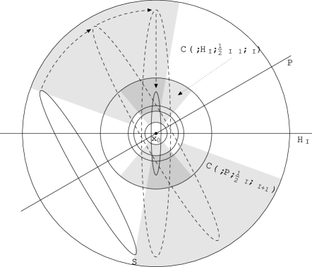
Figure 6. First we move the center of $S$ to $x_{0}$. Then we rotate $S$ so that it is perpendicular to $H_{I}$. Finally we change the radius so that it is between $\frac{1}{2}\rho_{I-1}$ and $\rho_{I}$.

We know that $F_{I+1}$ contains the conical cap $CC:=\mathbb{C}(\delta,P,\tfrac{1}{2}\rho_{I},\rho_{I+1})$, so we can use Proposition 1.29 to move $S$ inside $CC$, so that it is centered at the origin.

From (58) we get

$$\Sigma\cap\mathbb{A}(\tfrac{1}{2}\rho_{I},2\rho_{I})\subseteq\mathbb{R}^{n}\setminus\mathbb{C}(2h_{0}\delta,P)\subseteq\mathbb{C}(\sqrt{1-(2h_{0}\delta)^{2}},P^{\perp})\,.$$

Using this and our inductive assumption we obtain

$$\Sigma\cap\mathbb{A}(\tfrac{1}{2}\rho_{I},\rho_{I})\subseteq\mathbb{C}(\sqrt{1-\delta^{2}},H_{I}^{\perp})\cap\mathbb{C}(\sqrt{1-(2h_{0}\delta)^{2}},P^{\perp})\,.$$

We have two cones that have nonempty intersection and we chose $h_{0}$ such that (56) holds, so we can apply Proposition 1.30 with $\alpha=\delta$ and $\beta=2h_{0}\delta$. Hence the intersection $\mathbb{C}(\delta,H_{I})\cap\mathbb{C}(\delta,P)$ contains the space $H_{I}^{\perp}$. Therefore

$$H_{I}^{\perp}\cap\mathbb{A}(\tfrac{1}{2}\rho_{I},\rho_{I+1})\subseteq\mathbb{C}(\delta,P,\tfrac{1}{2}\rho_{I},\rho_{I+1})\cap F_{I}\,.$$

Using Corollary 1.28 we can rotate $S$ inside $CC$, so that it lies in $H^{\perp}$. Then we decrease the radius of $S$ to the value e.g. $\tfrac{3}{4}\rho_{I}\in(\frac{1}{2}\rho_{I-1},\rho_{I})$. Applying the inductive assumption we obtain condition (53) for $i=I+1$.

The set $\Sigma$ is compact and $\rho_{i}$ grows geometrically, so our construction has to end eventually. Otherwise we would find arbitrary large spheres, which are linked with $\Sigma$ but this contradicts compactness. ∎

Proposition 2.8.

Let $\Sigma\in\mathcal{A}(\delta,m)$ be an admissible set, such that $\mathcal{E}_{p}(\Sigma)\leq E<\infty$ for some $p>m(m+2)$. Then the stopping distances $d(x_{0})$ defined in Proposition 2.5 have a positive lower bound

(59) $$d(\Sigma):=\inf_{x_{0}\in\Sigma^{*}}d(x_{0})\geq\left(\frac{\hbox{}\hbox{}{{\mbox{{C\textsuperscript{st}{??}}}}}\hbox{}\hbox{}{{\mbox{{C\textsuperscript{st}{??}}}}}^{p}}{E}\right)^{\frac{1}{p-m(m+2)}}\,.$$

where $\hbox{}\hbox{}{{\mbox{{C\textsuperscript{st}{??}}}}}=\hbox{}\hbox{}{{\mbox{{C\textsuperscript{st}{??}}}}}(\delta,m)$ and $\hbox{}\hbox{}{{\mbox{{C\textsuperscript{st}{??}}}}}=\hbox{}\hbox{}{{\mbox{{C\textsuperscript{st}{??}}}}}(\delta,m)$ are some positive constants which depend only on $\delta$ and $m$.

Proof.

From Proposition 2.3 we know that $d(\Sigma)$ must satisfy (43) with the constant $A_{\Sigma}$ and $\eta=\eta(\delta,m)$ defined in (57). Hence, we already have a positive lower bound on $d(\Sigma)$. Now we only need to show that it does not depend on $A_{\Sigma}$.

Fix a point $x_{0}\in\Sigma^{*}$ such that $d(x_{0})<(1+\varepsilon)d(\Sigma)$ for some small $\varepsilon>0$. Proposition 2.5 gives us a simplex $T=\operatorname{\bigtriangleup}(x_{0},\ldots,x_{m+1})\in\mathcal{V}_{m}(\eta,d(x_{0}))$. From Proposition 1.45 we know that there exists a small number $\varsigma_{m}<\tfrac{1}{2}$ such that $T^{\prime}\in\mathcal{V}_{m}(\tfrac{1}{2}\eta,\tfrac{3}{2}d(x_{0}))$ for each $T^{\prime}=\operatorname{\bigtriangleup}(x_{0}^{\prime},\ldots,x_{m+1}^{\prime})$ satisfying $|x_{i}-x_{i}^{\prime}|\leq\varsigma_{m}d(x_{0})$ for $i=0,\ldots,m+1$. If $\varepsilon<\frac{1}{\varsigma_{m}}-1$ then

$$\varsigma_{m}d(x_{0})\leq\varsigma_{m}(1+\varepsilon)d(\Sigma)\leq d(\Sigma)\leq d(x_{i})\,,$$

so Corollary 2.6 gives us

$$\mathscr{H}^{m}(\Sigma\cap\mathbb{B}(x_{i},\varsigma_{m}d(x_{0})))\geq(1-\delta^{2})^{\frac{m}{2}}\omega_{m}(\varsigma_{m}d(x_{0}))^{m}\,.$$

Now, we can repeat the calculation from the proof of Proposition 2.3, replacing $A_{\Sigma}$ by $A_{1}=A_{1}(\delta,m):=\sqrt{1-\delta^{2}}\omega_{m}\varsigma_{m}^{m}$ to obtain

$$(1+\varepsilon)d(\Sigma)>d(x_{0})\geq\left(\frac{\hbox{}\hbox{}{{\mbox{{C\textsuperscript{st}{??}}}}}\hbox{}\hbox{}{{\mbox{{C\textsuperscript{st}{??}}}}}^{p}A_{1}^{m+2}\eta^{m(m+1)^{2}(m+2)}(\eta^{m+1})^{p}}{E}\right)^{\frac{1}{p-m(m+2)}}\,.$$

The constants $A_{1}$ and $\eta$ depend only on $\delta$ and $m$ so setting

C^st?? $$=\hbox{}\hbox{}{{\mbox{{C\textsuperscript{st}{??}}}}}(\delta,m):=\hbox{}\hbox{}{{\mbox{{C\textsuperscript{st}{??}}}}}(m)A_{1}(\delta,m)\eta(\delta,m)^{m(m+1)^{2}(m+2)}$$

andC^st?? $$=\hbox{}\hbox{}{{\mbox{{C\textsuperscript{st}{??}}}}}(\delta,m):=\hbox{}\hbox{}{{\mbox{{C\textsuperscript{st}{??}}}}}(m)\eta(\delta,m)^{m+1}$$

and letting $\varepsilon\to 0$ we reach the estimate (59). ∎

Proposition 2.9.

Let $\Sigma\in\mathcal{A}(\delta,m)$, $E>0$ and $p>m(m+2)$. Assume that $\mathcal{E}_{p}(\Sigma)\leq E<\infty$. Set

(60) $$\hbox{}\hbox{}{{\mbox{{C\textsuperscript{st}{??}}}}}=\hbox{}\hbox{}{{\mbox{{C\textsuperscript{st}{??}}}}}(E,m,p,\delta):=\left(\frac{\hbox{}\hbox{}{{\mbox{{C\textsuperscript{st}{??}}}}}\hbox{}\hbox{}{{\mbox{{C\textsuperscript{st}{??}}}}}^{p}}{E}\right)^{\frac{1}{p-m(m+2)}}\,.$$

Then for each $x\in\Sigma$ and $\rho\leq\hbox{}\hbox{}{{\mbox{{C\textsuperscript{st}{??}}}}}$ there exists an $m$-plane $H=H(\rho)\in G(n,m)$ such that

$$(x+H)\cap\mathbb{B}(x,\sqrt{1-\delta^{2}}\rho)\subseteq\pi_{x+H}(\Sigma\cap\mathbb{B}(x,\rho))\,.$$

Proof.

Proposition 2.5 gives us this result for any $x\in\Sigma^{*}$. We only need to show that it is true also for $x\in\Sigma\setminus\Sigma^{*}$.

Let $x$ be a point in $\Sigma\setminus\Sigma^{*}$ and fix a radius $\rho\leq\hbox{}\hbox{}{{\mbox{{C\textsuperscript{st}{??}}}}}$. Choose a sequence of points $x_{i}\in\Sigma^{*}$ converging to $x$. From Proposition 2.5 we obtain a sequence of $m$-planes $H_{i}\in G(n,m)$ such that

$$D_{i}:=(x_{i}+H_{i})\cap\mathbb{B}(x_{i},\sqrt{1-\delta^{2}}\rho)\subseteq\pi_{x_{i}+H_{i}}(\Sigma\cap\mathbb{B}(x_{i},\rho))\,.$$

Since the Grassmannian $G(n,m)$ is a compact manifold, passing to a subsequence we can assume that $H_{i}$ converges to some $H$ in $G(n,m)$. Set

$$D:=(x+H)\cap\mathbb{B}(x,\sqrt{1-\delta^{2}}\rho)\,.$$

Fix a point $w\in D$. We will show that the preimage $\pi_{x+H}^{-1}(w)\cap(\Sigma\cap\mathbb{B}(x,\rho))$ is nonempty. Chose points $w_{i}\in D_{i}$ such that $|w_{i}-x_{i}|=|w-x|$ and $w_{i}\to w$. We know that there exist points $y_{i}\in\Sigma\cap\mathbb{B}(x_{i},\rho)$ such that

$$\pi_{x_{i}+H_{i}}(y_{i})=w_{i}\,,$$

so

$$y_{i}=w_{i}+v_{i}\quad\text{for some }v_{i}\in H_{i}^{\perp}\,.$$

Moreover

$$\rho^{2}\geq|w_{i}-x_{i}|^{2}+|v_{i}|^{2}\,,$$

hence

$$|v_{i}|^{2}\leq\rho^{2}-|w_{i}-x_{i}|^{2}=\rho^{2}-|w-x|^{2}\,.$$

We now know that $v_{i}$ all lie inside a ball of radius $\rho^{2}-|w-x|^{2}$, which is compact, so passing to a subsequence, we can assume that $v_{i}\to v\in H^{\perp}$. This gives us

$$y_{i} =w_{i}+v_{i}\to y=w+v\,,$$

$$|v|^{2} \leq\rho^{2}-|w-x|^{2}$$

$$\text{and}\quad|y-x|^{2} =|w-x|^{2}+|v|^{2}\leq\rho\quad\Rightarrow\quad y\in\Sigma\cap\mathbb{B}(x,\rho)\,.$$

We have found $y\in\Sigma\cap\mathbb{B}(x,\rho)$ such that $\pi_{x+H}(y)=w$ and this completes the proof. ∎

Proof of Theorem 2.1.

We proceed as in the proof of Corollary 2.6. Orthogonal projections are Lipschitz mappings with constant $1$ so they cannot increase the measure. From Proposition 2.9 we know that for each $x\in\Sigma$ and each $\rho\leq\hbox{}\hbox{}{{\mbox{{C\textsuperscript{st}{??}}}}}=\hbox{}\hbox{}{{\mbox{{C\textsuperscript{st}{??}}}}}(E,m,p,\delta)$ there exists an $m$-plane $H$ such that the image of $\Sigma\cap\mathbb{B}(x,\rho)$ under $\pi_{x+H}$ contains the ball $(x+H)\cap\mathbb{B}(x,\sqrt{1-\delta^{2}}\rho)$. The measure of that ball is $(1-\delta^{2})^{\frac{m}{2}}\omega_{m}\rho^{m}$ so the $\mathscr{H}^{m}$-measure of $\Sigma\cap\mathbb{B}(x,\rho)$ cannot be less than this number. ∎

2.3. Relation between admissible sets and fine sets

In this paragraph we establish a connection between the class $\mathcal{A}(\delta,m)$ of admissible sets and the class $\mathcal{F}(m)$ of fine sets. We show (Theorem 2.13) that in the class of sets with finite $p$-energy every admissible set is also fine. Later in §3 we show that $m$-fine sets with bounded $p$-energy are $C^{1,\tau}$ manifolds, hence they are also $(\delta,m)$-admissible for any $\delta\in(0,1)$ (cf. Example 1.57).

Proposition 2.10.

Let $\Sigma\in\mathcal{A}(\delta,m)$ be $(\delta,m)$-admissible set for some $\delta\in(0,1)$ such that $\mathcal{E}_{p}(\Sigma)<\infty$ for some $p>m(m+2)$. Choose any number $L$ such that

$$\sqrt{\frac{2-\delta}{\delta}}<L<\frac{1}{\delta}\,.$$

Then for each $x\in\Sigma$ and each $r\leq\hbox{}\hbox{}{{\mbox{{C\textsuperscript{st}{??}}}}}$ there exists an $m$-plane $H\in G(n,m)$ such that

1. $(x+\mathbb{C}(L\delta,H,\frac{5}{8}r,\frac{7}{8}r))\cap\Sigma=\emptyset$ and

2. the sphere $S:=\mathbb{S}(x,\frac{6}{8}r)\cap(x+H^{\perp})$ is linked with $\Sigma$.

Proof.

In the proof of 2.5 we have shown that analogous conditions hold for $x\in\Sigma^{*}$. We know that at each $x\in\Sigma^{*}$ and for each $r\leq\hbox{}\hbox{}{{\mbox{{C\textsuperscript{st}{??}}}}}$ there exists an $m$-plane $H_{x}\in G(n,m)$ such that

• $(x+\mathbb{C}(\delta,H_{x},\frac{1}{2}r,r))\cap\Sigma=\emptyset$ and

• the sphere $S:=\mathbb{S}(x,\frac{3}{4}r)\cap(x+H_{x}^{\perp})$ is linked with $\Sigma$.

Now we only need to show that we can pass to a limit. Fix a number $K$ satisfying $\sqrt{\frac{2-\delta}{\delta}}<K<L$ and fix $r\leq\hbox{}\hbox{}{{\mbox{{C\textsuperscript{st}{??}}}}}$, let $x\in\Sigma\setminus\Sigma^{*}$ and let $x_{k}\in\Sigma^{*}$ be a sequence of points converging to $x$. Using compactness of $G(n,m)$ and possibly passing to a subsequence we obtain a convergent sequence of $m$-planes $H_{k}$. Let $H_{0}$ be the limit of $H_{k}$. For any choice of $\zeta>0$ and $\xi>0$ we can find $k_{0}$ such that for $k>k_{0}$ we have

$$\operatorname{\varangle}(H_{k},H_{0})\leq\zeta\quad\text{and}\quad|x_{k}-x_{0}|\leq\xi\,.$$

Lemma 2.11 (Step 1).

There exists $\zeta=\zeta(\delta,K)$ such that whenever $\operatorname{\varangle}(H_{k},H_{0})\leq\zeta$ then

$$\mathbb{C}(K\delta,H_{0})\subseteq\mathbb{C}(\delta,H_{k})\,.$$

Proof.

Let $x\in\mathbb{C}(K\delta,H_{0})$. First we estimate $|\pi_{H_{k}}(x)|$.

$$|\pi_{H_{k}}(x)| \leq|\pi_{H_{k}}(\pi_{H_{0}}(x))|+|\pi_{H_{k}}(Q_{H_{0}}(x))|$$

$$\leq|\pi_{H_{0}}(x)|+\zeta|Q_{H_{0}}(x)|\leq|x|(\sqrt{1-(K\delta)^{2}}+\zeta)\,.$$

Now we can wite

$$|Q_{H_{k}}(x)|\geq|x|-|\pi_{H_{k}}(x)|\geq|x|(1-\sqrt{1-(K\delta)^{2}}-\zeta)\,.$$

Therefore, we need to find $\zeta>0$ such that $1-\sqrt{1-(K\delta)^{2}}-\zeta\geq\delta$. Let us calculate

$$1-\sqrt{1-(K\delta)^{2}}-\zeta\geq\delta\quad\iff\quad\zeta\leq 1-\delta-\sqrt{1-(K\delta)^{2}}\,.$$

The question remains whether $1-\delta-\sqrt{1-(K\delta)^{2}}$ is positive. Another calculation shows

$$1-\delta-\sqrt{1-(K\delta)^{2}}>0\quad\iff\quad\frac{2-\delta}{\delta}<K^{2}\,,$$

but this is exactly what we assumed about $K$. We can safely set

$$\zeta=\zeta(\delta,K):=1-\delta-\sqrt{1-(K\delta)^{2}}\,.$$

∎

Lemma 2.12 (Step 2).

There exists $\xi=\xi(K,L,\delta,r)$ such that whenever $|x_{k}-x_{0}|\leq\xi$ then for each $x\in\mathbb{R}^{n}$ such that $|x-x_{0}|\geq\tfrac{1}{2}r$

$$|Q_{H_{0}}(x-x_{0})|\geq L\delta|x-x_{0}|\quad\Rightarrow\quad|Q_{H_{0}}(x-x_{k})|\geq K\delta|x-x_{k}|\,.$$

In other words

$$(x_{0}+\mathbb{C}(L\delta,H_{0}))\setminus\mathbb{B}(x_{0},\tfrac{1}{2}R)\subseteq(x_{0}+\mathbb{C}(\delta,H_{0}))\cap(x_{k}+\mathbb{C}(K\delta,H_{0}))\,.$$

Proof.

Let $x\in(x_{0}+\mathbb{C}(L\delta,H_{0}))$ be such that $|x-x_{0}|\geq\tfrac{1}{2}r$. We then have

$$|Q_{H_{0}}(x-x_{k})|\geq|Q_{H_{0}}(x-x_{0})|-|x_{k}-x_{0}|\geq L\delta|x-x_{0}|-\xi\,.$$

We need to find $\xi>0$ such that $L\delta|x-x_{0}|-\xi\geq K\delta|x-x_{k}|$. Set

$$\xi=\xi(K,L,\delta,r):=\tfrac{1}{4}\delta(L-K)r\,.$$

We obtain

$$(1+K\delta)\xi \leq 2\xi\leq\delta(L-K)\tfrac{1}{2}r\leq\delta(L-K)|x-x_{0}|$$

$$\,\Rightarrow\quad|Q_{H_{0}}(x-x_{k})|\geq L\delta|x-x_{0}|-\xi\geq K\delta(|x-x_{0}|+\xi)\geq K\delta|x-x_{k}|$$

∎

Lemmas 2.11 and 2.12 give us a good choice of $\zeta$ and $\xi$. Shrinking $\xi$ if needed, we can assume that $\xi<\frac{1}{8}r$. Then we have

$$\overline{\mathbb{B}}(x_{0},\tfrac{1}{2}r)\cup\overline{\mathbb{B}}(x_{k},\tfrac{1}{2}r) \subseteq\overline{\mathbb{B}}(x_{0},\tfrac{5}{8}r)$$

$$\text{and}\quad\mathbb{B}(x_{0},r)\cap\mathbb{B}(x_{k},r) \supseteq\mathbb{B}(x_{0},\tfrac{7}{8}r)\,.$$

Hence, for each $k$ big enough

(61) $$x_{0}+\mathbb{C}(L\delta,H_{0},\tfrac{5}{8}r,\tfrac{7}{8}r)\subseteq x_{k}+\mathbb{C}(\delta,H_{k},\tfrac{1}{2}r,r)\,,$$

and we obtain the first required condition

$$x_{0}+\mathbb{C}(L\delta,H_{0},\tfrac{5}{8}r,\tfrac{7}{8}r)\cap\Sigma=\emptyset\,.$$

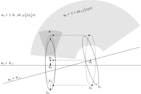
Figure 7. If $x_{k}$ is sufficiently close to $x_{0}$, then the cone over $x_{k}+H_{k}$ contains a small conical cap over $x_{0}+H_{0}$. This allows us to continuously transform $S_{1}$ into $S_{4}$ without leaving the grey area.

To prove the second condition, involving the linked spheres, let us set $S_{1}:=\mathbb{S}(x_{k},\tfrac{6}{8}r)\cap(x_{k}+H_{k}^{\perp})$. From the definition of admissible sets we know that $S_{1}$ is linked with $\Sigma$. We use Corollary 1.28 to find an isotopy (see Figure 7)

$$F_{1}:S_{1}\times[0,1]\to\big{(}x_{k}+\mathbb{C}(\delta,H_{k},\tfrac{1}{2}r,r)\big{)}\,,$$

which continuously rotates $S_{1}$ into $S_{2}:=\mathbb{S}(x_{k},\tfrac{6}{8}r)\cap(x_{k}+H_{0}^{\perp})$. All we need to know is that $S_{2}$ is contained in $x_{k}+\mathbb{C}(\delta,H_{k},\tfrac{1}{2}r,r)$ but this follows from Lemma 2.11. Next, we continuously translate $S_{2}$ into $S_{3}:=\mathbb{S}(y_{k},\tfrac{6}{8}r)\cap(y_{k}+H_{0}^{\perp})$, where $y_{k}:=x_{k}+\pi_{H_{0}}(x_{0}-x_{k})$, using the isotopy

$$F_{2}:S_{2}\times[0,1] \to\big{(}x_{k}+\mathbb{C}(\delta,H_{k},\tfrac{1}{2}r,r)\big{)}\,,$$

$$F_{2}(z,t) :=z+t\pi_{H_{0}}(x_{0}-x_{k})\,.$$

To see that this transformation is performed inside $x_{k}+\mathbb{C}(\delta,H_{k},\tfrac{1}{2}r,r)$ let us choose a point $z\in S_{2}$ and $t\in[0,1]$. Since $|\pi_{H_{0}}(x_{0}-x_{k})|\leq|x_{0}-x_{k}|\leq\xi$, we have $\frac{6}{8}r-\xi\leq|F_{2}(z,t)-x_{k}|\leq\frac{6}{8}r+\xi$ and

$$\frac{|Q_{H_{0}}(F_{2}(z,t)-x_{k})|}{|F_{2}(z,t)-x_{k}|}\geq\frac{\tfrac{6}{8}r}{\tfrac{6}{8}r+\xi}\geq\delta\iff\xi\leq\frac{6(1-\delta)}{8\delta}r\,.$$

To make everything work, we may shrink $\xi$, so that it satisfies the above condition. Finally we translate $S_{3}$ along the vector $Q_{H_{0}}(x_{0}-x_{k})$ into $S_{4}:=\mathbb{S}(x_{0},\tfrac{6}{8}r)\cap(x_{0}+H_{0}^{\perp})$ with the isotopy

$$F_{3}:S_{3}\times[0,1] \to H_{0}^{\perp}\cap\mathbb{A}(\tfrac{5}{8}r,\tfrac{7}{8}r)\,,$$

$$F_{3}(z,t) :=z+tQ_{H_{0}}(x_{0}-x_{k})\,.$$

We have $|Q_{H_{0}}(x_{0}-x_{k})|\leq\xi<\frac{1}{8}r$ and the last translation is performed inside $x_{0}+H_{0}^{\perp}$, so it stays in $x_{0}+\mathbb{C}(L\delta,H_{0},\tfrac{5}{8}r,\tfrac{7}{8}r)$. This gives the second condition of Proposition 2.10. ∎

Theorem 2.13.

If $\Sigma\subseteq\mathbb{R}^{n}$ is $(\delta,m)$-admissible and additionally $\mathcal{E}_{p}(\Sigma)\leq E<\infty$ for some $p>m(m+2)$, then $\Sigma$ is also $m$-fine with constants

$$A_{\Sigma}=(1-\delta^{2})^{m/2}\omega_{m}\,,\quad R_{\Sigma}=\min\{\hbox{}\hbox{}{{\mbox{{C\textsuperscript{st}{??}}}}},{R}_{2}(E,m,p,\delta)\}\quad and\quad M_{\Sigma}=5\,.$$

Proof.

To prevent confusion let us make the following distinction. In the proof we refer to constants from the definition of $(\delta,m)$-admissible sets by $A_{\Sigma}^{\prime}$ and $R_{\Sigma}^{\prime}$. The constants from the definition of $m$-fine sets we shall denote by $A_{\Sigma}$, $R_{\Sigma}$ and $M_{\Sigma}$.

Corollary 2.2 states that $A_{\Sigma}^{\prime}=(1-\delta^{2})^{m/2}\omega_{m}$ and $R_{\Sigma}^{\prime}=\hbox{}\hbox{}{{\mbox{{C\textsuperscript{st}{??}}}}}$, so these constants depend only on $E$, $m$, $p$ and $\delta$. Therefore we may set $A_{\Sigma}=A_{\Sigma}^{\prime}$ and then all we need to show is that there exist numbers $R_{\Sigma}\leq R_{\Sigma}^{\prime}$ and $M_{\Sigma}$ such that for $r\leq R_{\Sigma}$ and for all $x\in\Sigma$

$$\bar{\theta}_{m}(x,r)\leq M_{\Sigma}\bar{\beta}_{m}(x,r)\,.$$

From Corollary 2.4 we know that $\bar{\beta}_{m}(x,r)\leq\hbox{}\hbox{}{{\mbox{{C\textsuperscript{st}{??}}}}}E^{1/\kappa}r^{\tau}$, so it converges to $0$ when $r\to 0$ uniformly with respect to $x\in\Sigma$. Fix a point $x_{0}\in\Sigma$ and a radius $r\leq\hbox{}\hbox{}{{\mbox{{C\textsuperscript{st}{??}}}}}$. Choose some $m$-plane $P\in G(n,m)$ such that

$$\forall y\in\Sigma\cap\mathbb{B}(x_{0},r)\ \ |Q_{P}(y-x_{0})|\leq\bar{\beta}_{m}(x,r)\,.$$

Fix a number $L$ such that $\sqrt{\frac{2-\delta}{\delta}}<L<\frac{1}{\delta}$ and set

$$\beta:=2\bar{\beta}_{m}(x_{0},r)\qquad\text{and}\qquad\gamma:=\sqrt{1-(L\delta)^{2}}\in(0,1)\,.$$

Let $H$ be the $m$-plane for the point $x_{0}$ given by Proposition 2.10, so that

$$\mathbb{C}(L\delta,H,\tfrac{5}{8}r,\tfrac{7}{8}r)\cap\Sigma=\emptyset\,.$$

Let $z\in\Sigma\cap\mathbb{B}(x_{0},r)$ be any point in the intersection $\Sigma\cap\mathbb{B}(y,L\delta\frac{7}{8}r)\cap(y+H^{\perp})$, where $y$ is any point such that $(y-x_{0})\in H$ and $|y-x_{0}|=\frac{7}{8}r\gamma$. Such point $z$ exists since the sphere $\mathbb{S}(y,L\delta\frac{7}{8}r)\cap(y+H^{\perp})$ is linked with $\Sigma$ (cf. Lemma 1.11).

Note that $\frac{7}{8}r\gamma\leq|z-x_{0}|\leq\frac{7}{8}r$, so

$$\frac{|Q_{P}(z-x_{0})|}{|z-x_{0}|}\leq\frac{\beta r}{\tfrac{7}{8}r\gamma}=\frac{8\beta}{7\gamma}\,,$$

hence

$$(z-x_{0})\in\mathbb{C}\left(\big{(}1-\tfrac{(8\beta)^{2}}{(7\gamma)^{2}}\big{)}^{\frac{1}{2}},P^{\perp}\right)\cap\mathbb{C}(\gamma,H^{\perp})\,.$$

To apply Proposition 1.30 we need to ensure the condition

(62) $$\sqrt{1-\gamma^{2}}+\tfrac{8\beta}{7\gamma} \leq(1-\tfrac{8\beta}{7\gamma})\sqrt{1-\left(\tfrac{8\beta}{7\gamma}\right)^{2}}\iff$$

$$\iff\beta \leq\tfrac{7}{8}\gamma\left((1-\tfrac{8\beta}{7\gamma})\sqrt{1-\left(\tfrac{8\beta}{7\gamma}\right)^{2}}-\sqrt{1-\gamma^{2}}\right)\,.$$

Substituting $\Psi:=\frac{8\beta}{7\gamma}$ in (62) and recalling that $\gamma=\sqrt{1-(L\delta)^{2}}$ we obtain the following inequality

(63) $$\Psi\leq(1-\Psi)\sqrt{1-\Psi^{2}}-L\delta\,.$$

Note that if $\Psi\to 0$ then the right-hand side converges to $1-L\delta>0$. Let $\Psi_{0}$ be the smallest, positive root of the equation $\Psi=(1-\Psi)\sqrt{1-\Psi^{2}}-L\delta$. Then any $\Psi\in(0,\Psi_{0})$ satisfies (63). Recall that $\tfrac{1}{2}\beta=\bar{\beta}_{m}(x,r)\leq\hbox{}\hbox{}{{\mbox{{C\textsuperscript{st}{??}}}}}E^{1/\kappa}r^{\tau}$, so to ensure condition (62) it suffices to impose the following constraint

(64) $$r\leq\hbox{}\hbox{}{{\mbox{{C\textsuperscript{st}{??}}}}}(E,m,p,\delta):=\Bigg{(}\frac{7\gamma\Psi_{0}}{16\hbox{}\hbox{}{{\mbox{{C\textsuperscript{st}{??}}}}}}\Bigg{)}^{1/\tau}E^{-1/\lambda}\,.$$

Now, for such $r$ we can use Proposition 1.30 to obtain

$$H^{\perp}\subseteq\mathbb{C}(L\delta,H)\cap\mathbb{C}(\tfrac{8\beta}{7\gamma},P)\,.$$

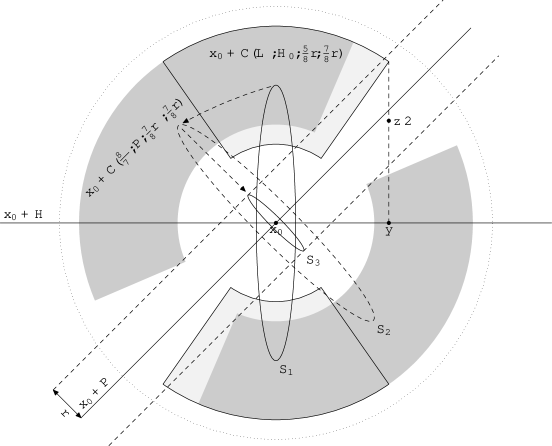
Figure 8. If $\beta$ is small enough, then the cone $\mathbb{C}(\tfrac{8\beta}{7\gamma},P)$ contains $H^{\perp}$ and we can continuously transform $S_{1}$ into $S_{3}$ inside the conical cap $\mathbb{C}(\tfrac{8\beta}{7\gamma},P,\frac{7}{8}r\gamma,\frac{7}{8}r)$.

Set $S_{1}:=\mathbb{S}(x_{0},\frac{7}{16}r(\gamma+1))\cap(x_{0}+H^{\perp})$. This sphere is contained in the conical cap $\mathbb{C}(\tfrac{8\beta}{7\gamma},P,\frac{7}{8}r\gamma,\frac{7}{8}r)$ (see Figure 8). Using Corollary 1.28 we rotate $S_{1}$ into $S_{2}:=\mathbb{S}(x_{0},\frac{7}{16}r(\gamma+1))\cap(x_{0}+P^{\perp})$ inside $\mathbb{C}(\tfrac{8\beta}{7\gamma},P,\frac{7}{8}r\gamma,\frac{7}{8}r)$. Note that for $x\in\Sigma$ such that $|x-x_{0}|>\frac{7}{8}r\gamma$ we have

$$\frac{Q_{P}(x-x_{0})}{|x-x_{0}|}<\frac{\beta r}{\frac{7}{8}r\gamma}=\frac{8\beta}{7\gamma}\,,$$

hence the conical cap $\mathbb{C}(\tfrac{8\beta}{7\gamma},P,\frac{7}{8}r\gamma,\frac{7}{8}r)$ does not intersect $\Sigma$ and the resulting sphere $S_{2}$ is still linked with $\Sigma$. Next we decrease the radius of $S_{2}$ to the value $\beta r$ obtaining another sphere $S_{3}:=\mathbb{S}(x_{0},\beta r)\cap(x_{0}+P^{\perp})$ which is also linked with $\Sigma$.

We can translate $S_{3}$ along any vector $v\in P$ with $|v|\leq\sqrt{1-\beta^{2}}r$ without changing the linking number. This way we see that for any point $w\in(x_{0}+P)\cap\overline{\mathbb{B}}(x_{0},\sqrt{1-\beta^{2}}r)$ there exists a point $z\in\Sigma$ such that $|z-w|\leq\beta r$.

For any other point $w\in(x_{0}+P)$ with $\sqrt{1-\beta^{2}}r\leq|w-x_{0}|\leq r$ we set

$$\tilde{w}:=w-(w-x_{0})|w-x_{0}|^{-1}(1-\sqrt{1-\beta^{2}})r\,,$$

so that $|\tilde{w}-x_{0}|\leq\sqrt{1-\beta^{2}}r$. Then we find $z\in\Sigma$ such that $|\tilde{w}-z|\leq\beta r$ and we obtain the estimate

$$|z-w| \leq|z-\tilde{w}|+|\tilde{w}-w|\leq\beta r+(1-\sqrt{1-\beta^{2}})r$$

$$=r\left(\beta+\frac{\beta^{2}}{1+\sqrt{1-\beta^{2}}}\right)\leq 2\beta r=4\bar{\beta}_{m}(x,r)r\,.$$

This implies that $d_{\mathcal{H}}(\Sigma\cap\overline{\mathbb{B}}(x_{0},r),(x_{0}+P)\cap\overline{\mathbb{B}}(x_{0},r))\leq 5\bar{\beta}_{m}(x_{0},r)$. Therefore the infimum over all $H\in G(n,m)$ must be even smaller, so $\bar{\theta}_{m}(x_{0},r)\leq 5\bar{\beta}_{m}(x_{0},r)$ for any $r\leq R_{\Sigma}$ and we can safely set $M_{\Sigma}:=5$. ∎

3. Existence and oscillation of tangent planes

In this paragraph we prove that boundedness of the $p$-energy $\mathcal{E}_{p}(\Sigma)\leq E$ implies $C^{1,\tau}$ regularity for some $\tau\in(0,1)$. First we show how to use the result (Proposition 1.39) obtained by David, Kenig and Toro [5] which immediately gives $C^{1,\tau}$ regularity. Then, independently of [5] we prove a bit stronger result (Theorem 3.2). We adjust the technique presented in [5] to our needs. We also carefully keep track of all the emerging constants and their dependences to be able to bound the Hölder norm and the size of the maps in terms of $E$ and independently of $\Sigma$.

Proposition 3.1.

Let $\Sigma\in\mathcal{F}(m)$ be such that $\mathcal{E}_{p}(\Sigma)\leq E<\infty$. Then $\Sigma$ is a closed $C^{1,\tau}$-submanifold of $\mathbb{R}^{n}$.

Proof.

From Corollary 2.4 we already have good estimates on the $\bar{\beta}_{m}$-numbers of $\Sigma$. Namely, for any $r<R_{\Sigma}$ and all $x\in\Sigma$ we have

$$\bar{\beta}_{m}(x,r)\leq\hbox{}\hbox{}{{\mbox{{C\textsuperscript{st}{??}}}}}E^{\frac{1}{\kappa}}r^{\tau}\,,$$

where C^st?? depends only on $m$, $p$ and $A_{\Sigma}$ and $\tau>0$. Since $\Sigma\in\mathcal{F}(m)$ it satisfies the condition II, so for $r<R_{\Sigma}$ we have

(65) $$\bar{\theta}_{m}(x,r)\leq\hbox{}\hbox{}{{\mbox{{C\textsuperscript{st}{??}}}}}M_{\Sigma}r^{\tau}\,,$$

which converges to $0$ when $r\to 0$ uniformly for all $x\in\Sigma$. Proposition 1.35 implies that $\theta_{m}(x,r)$ also converges uniformly to $0$ when $r\to 0$ and that $\beta_{m}(x,r)\lesssim r^{\tau}$ for each $x$ and $r<R_{\Sigma}$. Hence, $\Sigma$ is Reifenberg flat with vanishing constant and satisfies the assumptions of Proposition 1.39. Therefore $\Sigma$ is a $C^{1,\tau}$ manifold.

Assume that $\Sigma$ is not closed, so $\partial\Sigma\neq\emptyset$. Let $x\in\partial\Sigma$ be a boundary point. For $r$ small enough the set $\Sigma\cap\mathbb{B}(x,r)$ is close to some half-$m$-plane $H_{+}\simeq\mathbb{R}^{m-1}\times\mathbb{R}_{+}$. Then one sees easily that $\bar{\theta}_{m}(x,r)\geq 1$, but this contradicts estimate (65). ∎

The rest of this section is devoted to showing that $\Sigma\in\mathcal{F}(m)$ with $p$-energy bounded by $E<\infty$ has an atlas of maps of a given size, which depends only on $E$, $m$ and $p$ but not on $\Sigma$ itself. Moreover we show that $\Sigma$ is locally a graph of a $C^{1,\tau}$ function with the Hölder constant also depending only on the energy $E$, the dimension $m$ and the exponent $p$. In a forthcoming project, we plan use these results to address the following problem:

In the class of sets $\Sigma\in\mathcal{F}(m)$, normalized so that $0\in\Sigma$ and $\mathscr{H}^{m}(\Sigma)\leq 1$, with uniformly bounded $p$-energy $\mathcal{E}_{p}(\Sigma)\leq E$ for some $p>m(m+2)$ there can be only finite number of non-homeomorphic sets and the number of homeomorphism classes can be bounded in terms of $E$.

For the sake of brevity we introduce the following notation

$$\pi_{x}:=\pi_{T_{x}\Sigma}\qquad\text{and}\qquad Q_{x}:=Q_{T_{x}\Sigma}\,,$$

where $x\in\Sigma$. The main result of this section is

Theorem 3.2.

Let $\Sigma\in\mathcal{F}(m)$ be an $m$-fine set such that $\mathcal{E}_{p}(\Sigma)\leq E<\infty$ for some $p>m(m+2)$. Then $\Sigma$ is a smooth manifold of class $C^{1,\tau}$, where $\tau$ was defined in §2.1 by the formula

$$\tau=\tfrac{\lambda}{\kappa}=\tfrac{p-m(m+2)}{(m+1)(m(m+1)(m+2)+p)}\,.$$

Moreover there exists a constant ${C}_{11}=\hbox{}\hbox{}{{\mbox{{C\textsuperscript{st}{??}}}}}(m,p)$ such that if we set ${R}_{3}:=\hbox{}\hbox{}{{\mbox{{C\textsuperscript{st}{??}}}}}E^{-1/\lambda}$ then for each point $x\in\Sigma$ there exists a $C^{1,\tau}$ function

$$F_{x}:T_{x}\Sigma\cap\overline{\mathbb{B}}_{\frac{1}{2}\hbox{}\hbox{}{{\mbox{{C\textsuperscript{st}{??}}}}}}\to T_{x}\Sigma^{\perp}\cap\overline{\mathbb{B}}_{\hbox{}\hbox{}{{\mbox{{C\textsuperscript{st}{??}}}}}}\,,$$

such that

$$(\Sigma-x)\cap\{y\in\overline{\mathbb{B}}_{\hbox{}\hbox{}{{\mbox{{C\textsuperscript{st}{??}}}}}}:|\pi_{x}(y)|\leq\tfrac{1}{2}\hbox{}\hbox{}{{\mbox{{C\textsuperscript{st}{??}}}}}\}=F_{x}(T_{x}\Sigma\cap\overline{\mathbb{B}}_{\frac{1}{2}\hbox{}\hbox{}{{\mbox{{C\textsuperscript{st}{??}}}}}})\,,$$

$$F_{x}(0)=0\qquad\text{and}\qquad DF_{x}(0)=0\,.$$

Furthermore there exists a constant ${C}_{12}=\hbox{}\hbox{}{{\mbox{{C\textsuperscript{st}{??}}}}}(m,p)$ such that for any two points $w_{0},w_{1}\in T_{x}\Sigma\cap\overline{\mathbb{B}}_{\frac{1}{2}\hbox{}\hbox{}{{\mbox{{C\textsuperscript{st}{??}}}}}}$ we have

$$\|DF_{x}(w_{1})-DF_{x}(w_{0})\|\leq\hbox{}\hbox{}{{\mbox{{C\textsuperscript{st}{??}}}}}E^{1/\kappa}|w_{1}-w_{0}|^{\tau}\,.$$

To prove this theorem we fix a point $x\in\Sigma$ and for each radii $r>0$ we choose an $m$-plane $P(x,r)$. Then we use the fact that $\bar{\theta}_{m}(x,r)\leq M_{\Sigma}\bar{\beta}_{m}(x,r)\leq M_{\Sigma}\hbox{}\hbox{}{{\mbox{{C\textsuperscript{st}{??}}}}}E^{\frac{1}{\kappa}}r^{\tau}$ to show that $P(x,r)$ converge to the tangent plane $T_{x}\Sigma$, when $r\to 0$. This also gives a bound on the oscillation of $T_{x}\Sigma$. Then we derive Lemma 3.9, which says that at some small scale we cannot have two distinct points $y$ and $z$ of $\Sigma$ such that the vector $v=(y-z)$ is orthogonal to $T_{x}\Sigma$. Any such vector $v$ would be close to the tangent plane $T_{z}\Sigma$ and this would violate the bound on the oscillation of tangent planes proved earlier. From here, it follows that there exists a small radius C^st?? such that $\Sigma\cap\mathbb{B}(x,\hbox{}\hbox{}{{\mbox{{C\textsuperscript{st}{??}}}}})$ is a graph of some function $F_{x}$.

Next we define the differential $DF_{x}$ at a point $w\in T_{x}\Sigma\cap\overline{\mathbb{B}}(x,\hbox{}\hbox{}{{\mbox{{C\textsuperscript{st}{??}}}}})$ using the inverse of the projection from $T_{y}\Sigma$ onto $T_{x}\Sigma$, where $y=F_{x}(w)+w$. This can be done since $y$ lies in $\Sigma\cap\overline{\mathbb{B}}(x,\hbox{}\hbox{}{{\mbox{{C\textsuperscript{st}{??}}}}})$, so the ”angle” $\operatorname{\varangle}(T_{x}\Sigma,T_{y}\Sigma)$ is small and due to Remark 1.14 the projection $\pi_{x}$ gives a linear isomorphism between $T_{x}\Sigma$ and $T_{y}\Sigma$. After that it is easy to see that the oscillation of $DF_{x}$ is roughly the same as the oscillation of $T_{x}\Sigma$, so $DF_{x}$ is actually Hölder continuous.

3.1. The tangent planes

Set

(66) $${R}_{4}=\hbox{}\hbox{}{{\mbox{{C\textsuperscript{st}{??}}}}}(E,m,p,M_{\Sigma},A_{\Sigma},R_{\Sigma}) :=\min\left\{(4\hbox{}\hbox{}{{\mbox{{C\textsuperscript{st}{??}}}}}E^{1/\kappa}M_{\Sigma})^{-1/\tau},R_{\Sigma}\right\}$$

$$=\min\left\{(4\hbox{}\hbox{}{{\mbox{{C\textsuperscript{st}{??}}}}}M_{\Sigma})^{-1/\tau}E^{-1/\lambda},R_{\Sigma}\right\}$$

so that $\hbox{}\hbox{}{{\mbox{{C\textsuperscript{st}{??}}}}}E^{1/\kappa}\hbox{}\hbox{}{{\mbox{{C\textsuperscript{st}{??}}}}}^{\tau}\leq(4M_{\Sigma})^{-1}$. Then for any $r\leq\hbox{}\hbox{}{{\mbox{{C\textsuperscript{st}{??}}}}}$ we have

$$\bar{\theta}_{m}(x,r)\leq M_{\Sigma}\bar{\beta}_{m}(x,r)\leq M_{\Sigma}\hbox{}\hbox{}{{\mbox{{C\textsuperscript{st}{??}}}}}E^{1/\kappa}r^{\tau}\leq M_{\Sigma}\hbox{}\hbox{}{{\mbox{{C\textsuperscript{st}{??}}}}}E^{1/\kappa}\hbox{}\hbox{}{{\mbox{{C\textsuperscript{st}{??}}}}}^{\tau}\leq\tfrac{1}{4}\,.$$

Lemma 3.3.

Choose a point $x\in\Sigma$ and fix some $r_{0}\leq\hbox{}\hbox{}{{\mbox{{C\textsuperscript{st}{??}}}}}$. Choose another point $y\in\Sigma\cap\overline{\mathbb{B}}(x,\frac{1}{2}r_{0})$ and some $r_{1}\in\left[\frac{1}{2}r_{0},r_{0}-|x-y|\right]$. Let $H_{0}\in\operatorname{BAP_{m}}(x,r_{0})$ and $H_{1}\in\operatorname{BAP_{m}}(y,r_{1})$. Then

$$\operatorname{\varangle}(H_{0},H_{1})\leq{C}_{13}E^{1/\kappa}r_{0}^{\tau}\,,$$

where $\hbox{}\hbox{}{{\mbox{{C\textsuperscript{st}{??}}}}}=\hbox{}\hbox{}{{\mbox{{C\textsuperscript{st}{??}}}}}(m,p,M_{\Sigma},A_{\Sigma})$.

Figure 9. The existence of $z\in\Sigma$ is guaranteed by the condition $\bar{\theta}_{m}(x,r)\leq M_{\Sigma}\bar{\beta}_{m}(x,r)$. This allows us to estimate $\operatorname{\varangle}(H_{0},H_{1})$.

Proof.

Set $\beta_{0}:=\bar{\beta}_{m}(x,r_{0})$ and $\beta_{1}:=\bar{\beta}_{m}(y,r_{1})$. Let $v\in H_{1}$ be any vector of length $|v|=r_{1}(1-M_{\Sigma}\beta_{1})$. Since $\bar{\theta}_{m}(y,r_{1})\leq M_{\Sigma}\beta_{1}$, there exists a point $z\in\Sigma\cap\overline{\mathbb{B}}(y+v,M_{\Sigma}\beta_{1}r_{1})$. Hence $|(y+v)-z|\leq M_{\Sigma}\beta_{1}r_{1}$ (see Figure 9). Note that $\overline{\mathbb{B}}(y+v,M_{\Sigma}\beta_{1}r_{1})\subseteq\overline{\mathbb{B}}(y,r_{1})\subseteq\overline{\mathbb{B}}(x,r_{0})$. Therefore $\operatorname{dist}(z,x+H_{0})=|Q_{H_{0}}(z-x)|\leq\beta_{0}r_{0}$ and we obtain the estimate

$$|Q_{H_{0}}(v)| \leq|Q_{H_{0}}((y-x)+v)|+|Q_{H_{0}}(y-x)|$$

$$\leq|((y-x)+v)-(z-x)|+|Q_{H_{0}}(z-x)|+|Q_{H_{0}}(y-x)|$$

$$\leq M_{\Sigma}\beta_{1}r_{1}+\beta_{0}r_{0}+\beta_{0}r_{0}\leq(M_{\Sigma}+2)\hbox{}\hbox{}{{\mbox{{C\textsuperscript{st}{??}}}}}E^{1/\kappa}r_{0}^{1+\tau}\,.$$

Since $v$ was chosen arbitrarily we get the following estimate for any unit vector $e\in H_{1}\cap\mathbb{S}$

$$|Q_{H_{0}}(e)|\leq(M_{\Sigma}+2)\hbox{}\hbox{}{{\mbox{{C\textsuperscript{st}{??}}}}}E^{1/\kappa}\frac{r_{0}^{1+\tau}}{r_{1}(1-M_{\Sigma}\beta_{1})}\leq(M_{\Sigma}+2)\hbox{}\hbox{}{{\mbox{{C\textsuperscript{st}{??}}}}}E^{1/\kappa}\frac{4r_{0}^{1+\tau}}{3r_{1}}\,.$$

Recall that $r_{1}\geq\frac{1}{2}r_{0}$, so we have

$$|Q_{H_{0}}(e)|\leq\tfrac{8}{3}(M_{\Sigma}+2)\hbox{}\hbox{}{{\mbox{{C\textsuperscript{st}{??}}}}}E^{1/\kappa}r_{0}^{\tau}\,.$$

Applying Proposition 1.22 we get

$$\operatorname{\varangle}(H_{0},H_{1})\leq\tfrac{8}{3}(M_{\Sigma}+2)\hbox{}\hbox{}{{\mbox{{C\textsuperscript{st}{??}}}}}\hbox{}\hbox{}{{\mbox{{C\textsuperscript{st}{??}}}}}E^{1/\kappa}r_{0}^{\tau}\,.$$

Finally we set $\hbox{}\hbox{}{{\mbox{{C\textsuperscript{st}{??}}}}}:=\tfrac{8}{3}(M_{\Sigma}+2)\hbox{}\hbox{}{{\mbox{{C\textsuperscript{st}{??}}}}}\hbox{}\hbox{}{{\mbox{{C\textsuperscript{st}{??}}}}}$. ∎

Lemma 3.4.

Choose a point $x\in\Sigma$. For each $r\leq\hbox{}\hbox{}{{\mbox{{C\textsuperscript{st}{??}}}}}$ fix an $m$-plane $P(r)\in\operatorname{BAP_{m}}(x,r)$. There exists a limit

$$\lim_{r\to 0}P(r)=:T_{x}\Sigma\in G(n,m)$$

and it does not depend on the choice of $P(r)\in\operatorname{BAP_{m}}(x,r)$.

Proof.

Set $\rho_{k}:=2^{-k}\hbox{}\hbox{}{{\mbox{{C\textsuperscript{st}{??}}}}}$ and for each $k$ choose $P_{k}\in\operatorname{BAP_{m}}(x,\rho_{k})$. Set $\beta_{k}:=\bar{\beta}_{m}(x,\rho_{k})$. We will show that $\{P(r)\}_{r<\hbox{}\hbox{}{{\mbox{{C\textsuperscript{st}{??}}}}}}$ satisfies the Cauchy condition. Fix some $0<s<t<\rho_{0}$ and find two natural numbers $k<l$ such that $\rho_{l+1}<s\leq\rho_{l}$ and $\rho_{k+1}<t\leq\rho_{k}$.

Applying Lemma 3.3 with $x=y$, $r_{0}=\rho_{j}$ and $r_{1}:=\frac{1}{2}r_{0}=\rho_{j+1}$ we obtain

$$\operatorname{\varangle}(P_{j},P_{j+1})\leq\hbox{}\hbox{}{{\mbox{{C\textsuperscript{st}{??}}}}}E^{1/\kappa}\rho_{j}^{\tau}\,.$$

Setting $r_{0}:=\rho_{l}$ and $r_{1}:=s$ or $r_{0}:=\rho_{k}$ and $r_{1}:=t$ we also get

$$\operatorname{\varangle}(P(s),P_{l}) \leq\hbox{}\hbox{}{{\mbox{{C\textsuperscript{st}{??}}}}}E^{1/\kappa}\rho_{l}^{\tau}\,,$$

$$\operatorname{\varangle}(P(t),P_{k}) \leq\hbox{}\hbox{}{{\mbox{{C\textsuperscript{st}{??}}}}}E^{1/\kappa}\rho_{k}^{\tau}\,.$$

Using these estimates we can write

$$\operatorname{\varangle}(P(r),P(s)) \leq\operatorname{\varangle}(P(r),P_{k})+\sum_{j=k}^{l-1}\operatorname{\varangle}(P_{j},P_{j+1})+\operatorname{\varangle}(P_{l},P(s))$$

$$\leq\hbox{}\hbox{}{{\mbox{{C\textsuperscript{st}{??}}}}}E^{1/\kappa}\left(\rho_{k}^{\tau}+\sum_{j=k}^{l}\rho_{j}^{\tau}\right)=\hbox{}\hbox{}{{\mbox{{C\textsuperscript{st}{??}}}}}E^{1/\kappa}\rho_{k}^{\tau}\left(1+\sum_{j=0}^{l-k}2^{-j\tau}\right)$$

$$\leq\hbox{}\hbox{}{{\mbox{{C\textsuperscript{st}{??}}}}}E^{1/\kappa}\frac{2^{1+\tau}}{2^{\tau}-1}\rho_{k}^{\tau}=:{C}_{14}E^{1/\kappa}\rho_{k}^{\tau}\,,$$

which shows that the Cauchy condition is satisfied, so $P(r)$ converges in $G(n,m)$ to some $m$-plane, which we refer to as the tangent plane $T_{x}\Sigma$. The above estimates are valid for any choice of $P(r)\in\operatorname{BAP_{m}}(x,r)$, so we have actually shown that $T_{x}\Sigma$ not only exists but is also uniquely determined. ∎

Remark 3.5.

Note that

$$\hbox{}\hbox{}{{\mbox{{C\textsuperscript{st}{??}}}}}=\hbox{}\hbox{}{{\mbox{{C\textsuperscript{st}{??}}}}}(m,p,M_{\Sigma},A_{\Sigma})=\hbox{}\hbox{}{{\mbox{{C\textsuperscript{st}{??}}}}}\frac{2^{1+\tau}}{2^{\tau}-1}\,.$$

Corollary 3.6.

Choose a point $x\in\Sigma$. For any $r\leq\hbox{}\hbox{}{{\mbox{{C\textsuperscript{st}{??}}}}}$ and any $H\in\operatorname{BAP_{m}}(x,r)$ we have

$$\operatorname{\varangle}(T_{x}\Sigma,H)\leq\hbox{}\hbox{}{{\mbox{{C\textsuperscript{st}{??}}}}}E^{1/\kappa}r^{\tau}$$

Corollary 3.7.

Choose a point $x\in\Sigma$. For any $y\in\Sigma\cap\overline{\mathbb{B}}(x,\hbox{}\hbox{}{{\mbox{{C\textsuperscript{st}{??}}}}})$ we have

$$\operatorname{dist}(y,x+T_{x}\Sigma)=|Q_{x}(y-x)|\leq{C}_{15}E^{1/\kappa}|y-x|^{1+\tau}\,,$$

where $\hbox{}\hbox{}{{\mbox{{C\textsuperscript{st}{??}}}}}=\hbox{}\hbox{}{{\mbox{{C\textsuperscript{st}{??}}}}}(m,p,M_{\Sigma},A_{\Sigma})$. In particular

$$|Q_{x}(y-x)|\leq\hbox{}\hbox{}{{\mbox{{C\textsuperscript{st}{??}}}}}E^{1/\kappa}\hbox{}\hbox{}{{\mbox{{C\textsuperscript{st}{??}}}}}^{\tau}|y-x|\leq\frac{\hbox{}\hbox{}{{\mbox{{C\textsuperscript{st}{??}}}}}}{4\hbox{}\hbox{}{{\mbox{{C\textsuperscript{st}{??}}}}}M_{\Sigma}}|y-x|=:{C}_{16}|y-x|\,.$$

Proof.

Choose an $m$-plane $H\in\operatorname{BAP_{m}}(x,|y-x|)$. Then we have

$$|Q_{x}(y-x)| \leq|Q_{H}(y-x)|+|Q_{x}(\pi_{H}(y-x))|$$

$$\leq|y-x|\bar{\beta}_{m}(x,|y-x|)+|y-x|\hbox{}\hbox{}{{\mbox{{C\textsuperscript{st}{??}}}}}E^{1/\kappa}|y-x|^{\tau}$$

$$\leq\hbox{}\hbox{}{{\mbox{{C\textsuperscript{st}{??}}}}}E^{1/\kappa}|y-x|^{1+\tau}\,,$$

where $\hbox{}\hbox{}{{\mbox{{C\textsuperscript{st}{??}}}}}:=\hbox{}\hbox{}{{\mbox{{C\textsuperscript{st}{??}}}}}+\hbox{}\hbox{}{{\mbox{{C\textsuperscript{st}{??}}}}}$. This also gives

$$\hbox{}\hbox{}{{\mbox{{C\textsuperscript{st}{??}}}}}=\hbox{}\hbox{}{{\mbox{{C\textsuperscript{st}{??}}}}}(m,p,M_{\Sigma})=\frac{\hbox{}\hbox{}{{\mbox{{C\textsuperscript{st}{??}}}}}+\hbox{}\hbox{}{{\mbox{{C\textsuperscript{st}{??}}}}}}{4\hbox{}\hbox{}{{\mbox{{C\textsuperscript{st}{??}}}}}M_{\Sigma}}=\frac{\tfrac{8}{3}(M_{\Sigma}+2)\hbox{}\hbox{}{{\mbox{{C\textsuperscript{st}{??}}}}}\frac{2^{1+\tau}}{2^{\tau}-1}+1}{4M_{\Sigma}}\,.$$

∎

Lemma 3.8.

Choose any point $x\in\Sigma$. There exists a constant ${C}_{17}=\hbox{}\hbox{}{{\mbox{{C\textsuperscript{st}{??}}}}}(m,p,M_{\Sigma},A_{\Sigma})$ such that for each $y\in\Sigma\cap\overline{\mathbb{B}}(x,\tfrac{1}{2}\hbox{}\hbox{}{{\mbox{{C\textsuperscript{st}{??}}}}})$ we have

$$\operatorname{\varangle}(T_{x}\Sigma,T_{y}\Sigma)\leq\hbox{}\hbox{}{{\mbox{{C\textsuperscript{st}{??}}}}}E^{1/\kappa}|x-y|^{\tau}\,.$$

Proof.

Let $y\in\Sigma\cap\overline{\mathbb{B}}(x,\frac{1}{2}\hbox{}\hbox{}{{\mbox{{C\textsuperscript{st}{??}}}}})$. Set $r_{0}:=2|x-y|$ and $r_{1}=|x-y|$. Choose any $H_{0}\in\operatorname{BAP_{m}}(x,r_{0})$ and any $H_{1}\in\operatorname{BAP_{m}}(y,r_{1})$. From Lemma 3.3 we have

$$\operatorname{\varangle}(H_{0},H_{1})\leq\hbox{}\hbox{}{{\mbox{{C\textsuperscript{st}{??}}}}}E^{1/\kappa}r_{0}^{\tau}\,.$$

On the other hand Corollary 3.6 says that

$$\operatorname{\varangle}(T_{x}\Sigma,H_{0})\leq\hbox{}\hbox{}{{\mbox{{C\textsuperscript{st}{??}}}}}E^{1/\kappa}r_{0}^{\tau}\qquad\text{and}\qquad\operatorname{\varangle}(T_{y}\Sigma,H_{1})\leq\hbox{}\hbox{}{{\mbox{{C\textsuperscript{st}{??}}}}}E^{1/\kappa}r_{0}^{\tau}\,.$$

Putting these estimates together we obtain

$$\operatorname{\varangle}(T_{x}\Sigma,T_{y}\Sigma) \leq\operatorname{\varangle}(T_{x}\Sigma,H_{0})+\operatorname{\varangle}(H_{0},H_{1})+\operatorname{\varangle}(H_{1},T_{y}\Sigma)$$

$$\leq(\hbox{}\hbox{}{{\mbox{{C\textsuperscript{st}{??}}}}}+2\hbox{}\hbox{}{{\mbox{{C\textsuperscript{st}{??}}}}})E^{1/\kappa}r_{0}^{\tau}=\hbox{}\hbox{}{{\mbox{{C\textsuperscript{st}{??}}}}}E^{1/\kappa}|x-y|^{\tau}\,,$$

where $\hbox{}\hbox{}{{\mbox{{C\textsuperscript{st}{??}}}}}:=\hbox{}\hbox{}{{\mbox{{C\textsuperscript{st}{??}}}}}+2\hbox{}\hbox{}{{\mbox{{C\textsuperscript{st}{??}}}}}$. ∎

3.2. The parameterizing function $F_{x}$

Combining Corollary 3.7 and Lemma 3.8 one can see that if we have two distinct points $y,z\in\Sigma$ such that $y-z\perp T_{x}\Sigma$ and $|y-z|\lesssim|x-y|$ then the tangent plane $T_{y}\Sigma$ must form a large angle with the plane $T_{x}\Sigma$. Such situation can only happen far away from $x$ because of the bound on the oscillation of tangent planes. Hence we have the following

Lemma 3.9.

Choose any point $x\in\Sigma$. There exists a radius ${R}_{5}>0$ such that if $y,z\in\Sigma\cap\overline{\mathbb{B}}(x,\frac{1}{2}\hbox{}\hbox{}{{\mbox{{C\textsuperscript{st}{??}}}}})$ and $(y-z)\perp T_{x}\Sigma$, then necessarily $\max\{|x-y|,|x-z|\}>\hbox{}\hbox{}{{\mbox{{C\textsuperscript{st}{??}}}}}$.

Proof.

Choose two points $y,z\in\Sigma\cap\overline{\mathbb{B}}(x,\frac{1}{2}\hbox{}\hbox{}{{\mbox{{C\textsuperscript{st}{??}}}}})$ such that $(z-y)\perp T_{x}\Sigma$. Without loss of generality we can assume that $|x-y|\geq|x-z|$. First we estimate the distance $|y-z|$ using Corollary 3.7. We have

(67) $$|y-z|=|Q_{x}(y-z)| \leq|Q_{x}(y-x)|+|Q_{x}(x-z)|$$

$$\leq\hbox{}\hbox{}{{\mbox{{C\textsuperscript{st}{??}}}}}|y-x|+\hbox{}\hbox{}{{\mbox{{C\textsuperscript{st}{??}}}}}|x-z|\leq 2\hbox{}\hbox{}{{\mbox{{C\textsuperscript{st}{??}}}}}|x-y|\,.$$

Set $\tilde{\hbox{}\hbox{}{{\mbox{{C\textsuperscript{st}{??}}}}}}:=\frac{\hbox{}\hbox{}{{\mbox{{C\textsuperscript{st}{??}}}}}}{4\hbox{}\hbox{}{{\mbox{{C\textsuperscript{st}{??}}}}}}$. If $|x-y|\leq\tilde{\hbox{}\hbox{}{{\mbox{{C\textsuperscript{st}{??}}}}}}$, then $\hbox{}\hbox{}{{\mbox{{C\textsuperscript{st}{??}}}}}|x-y|\leq\tfrac{1}{2}\hbox{}\hbox{}{{\mbox{{C\textsuperscript{st}{??}}}}}$. Hence $|y-z|\leq\tfrac{1}{2}\hbox{}\hbox{}{{\mbox{{C\textsuperscript{st}{??}}}}}$ and we can use Corollary 3.7 once again to estimate the distance between $T_{y}\Sigma$ and $z$.

Using the definition of $\operatorname{\varangle}$ we may write

(68) $$\operatorname{\varangle}(T_{x}\Sigma,T_{y}\Sigma) \geq|z-y|^{-1}|\pi_{x}(z-y)-\pi_{y}(z-y)|=|z-y|^{-1}|\pi_{y}(z-y)|$$

$$\geq|z-y|^{-1}\left(|z-y|-|Q_{y}(z-y)|\right)$$

$$\geq|z-y|^{-1}\left(|z-y|-\hbox{}\hbox{}{{\mbox{{C\textsuperscript{st}{??}}}}}E^{1/\kappa}|z-y|^{1+\tau}\right)$$

$$=1-\hbox{}\hbox{}{{\mbox{{C\textsuperscript{st}{??}}}}}E^{1/\kappa}|z-y|^{\tau}\,.$$

On the other hand Lemma 3.8 gives us

(69) $$\operatorname{\varangle}(T_{x}\Sigma,T_{y}\Sigma)\leq\hbox{}\hbox{}{{\mbox{{C\textsuperscript{st}{??}}}}}E^{1/\kappa}|x-y|^{\tau}\,.$$

Putting these two estimates together we have

$$1-\hbox{}\hbox{}{{\mbox{{C\textsuperscript{st}{??}}}}}E^{1/\kappa}|z-y|^{\tau}\leq\operatorname{\varangle}(T_{x}\Sigma,T_{y}\Sigma)\leq\hbox{}\hbox{}{{\mbox{{C\textsuperscript{st}{??}}}}}E^{1/\kappa}|x-y|^{\tau}\,.$$

By (67),

$$1-\hbox{}\hbox{}{{\mbox{{C\textsuperscript{st}{??}}}}}E^{1/\kappa}(2\hbox{}\hbox{}{{\mbox{{C\textsuperscript{st}{??}}}}})^{\tau}|x-y|^{\tau}\leq\hbox{}\hbox{}{{\mbox{{C\textsuperscript{st}{??}}}}}E^{1/\kappa}|x-y|^{\tau}\,.$$

Hence

$$|x-y|\geq E^{-1/\lambda}(\hbox{}\hbox{}{{\mbox{{C\textsuperscript{st}{??}}}}}+\hbox{}\hbox{}{{\mbox{{C\textsuperscript{st}{??}}}}}(2\hbox{}\hbox{}{{\mbox{{C\textsuperscript{st}{??}}}}})^{\tau})^{-1/\tau}\,.$$

We may set

(70) $$\hbox{}\hbox{}{{\mbox{{C\textsuperscript{st}{??}}}}}=\hbox{}\hbox{}{{\mbox{{C\textsuperscript{st}{??}}}}}(E,m,p,M_{\Sigma},A_{\Sigma},R_{\Sigma}) :=\min\left\{\frac{1}{2}E^{-1/\lambda}(\hbox{}\hbox{}{{\mbox{{C\textsuperscript{st}{??}}}}}+\hbox{}\hbox{}{{\mbox{{C\textsuperscript{st}{??}}}}}(2\hbox{}\hbox{}{{\mbox{{C\textsuperscript{st}{??}}}}})^{\tau})^{-1/\tau},\tilde{\hbox{}\hbox{}{{\mbox{{C\textsuperscript{st}{??}}}}}}\right\}$$

$$=\min\left\{\frac{1}{2}E^{-1/\lambda}(\hbox{}\hbox{}{{\mbox{{C\textsuperscript{st}{??}}}}}+\hbox{}\hbox{}{{\mbox{{C\textsuperscript{st}{??}}}}}(2\hbox{}\hbox{}{{\mbox{{C\textsuperscript{st}{??}}}}})^{\tau})^{-1/\tau},\frac{\hbox{}\hbox{}{{\mbox{{C\textsuperscript{st}{??}}}}}}{4\hbox{}\hbox{}{{\mbox{{C\textsuperscript{st}{??}}}}}}\right\}\,.$$

∎

Let us define

(71) $$\hbox{}\hbox{}{{\mbox{{C\textsuperscript{st}{??}}}}}=\hbox{}\hbox{}{{\mbox{{C\textsuperscript{st}{??}}}}}(E,m,p,M_{\Sigma},A_{\Sigma},R_{\Sigma}):=\frac{1}{2}\min\{E^{-1/\lambda}(2\hbox{}\hbox{}{{\mbox{{C\textsuperscript{st}{??}}}}})^{-1/\tau},\hbox{}\hbox{}{{\mbox{{C\textsuperscript{st}{??}}}}},\tfrac{1}{2}\hbox{}\hbox{}{{\mbox{{C\textsuperscript{st}{??}}}}}\}\,.$$

This definition assures that for any $y,z\in\Sigma\cap\overline{\mathbb{B}}(x,\hbox{}\hbox{}{{\mbox{{C\textsuperscript{st}{??}}}}})$ we have

$$\operatorname{\varangle}(T_{y}\Sigma,T_{z}\Sigma)\leq\tfrac{1}{2}\,.$$

Here, the radius C^st?? depends on $A_{\Sigma}$, $M_{\Sigma}$ and $R_{\Sigma}$ but at the end of this section we shall prove that one can drop these dependencies just by showing that $A_{\Sigma}$, $M_{\Sigma}$ and $R_{\Sigma}$ can be expressed solely in terms if $E$, $m$ and $p$.

Corollary 3.10.

For each $x\in\Sigma$ and each $y\in\Sigma\cap\overline{\mathbb{B}}(x,\hbox{}\hbox{}{{\mbox{{C\textsuperscript{st}{??}}}}})$ the point $y$ is the only point in the intersection $\Sigma\cap(y+T_{x}\Sigma^{\perp})\cap\overline{\mathbb{B}}(x,\hbox{}\hbox{}{{\mbox{{C\textsuperscript{st}{??}}}}})$. Therefore $(\Sigma-x)\cap\overline{\mathbb{B}}_{\hbox{}\hbox{}{{\mbox{{C\textsuperscript{st}{??}}}}}}$ is a graph of the function

(72) $$F_{x}:\tilde{\mathcal{D}}_{x} \to T_{x}\Sigma^{\perp}\cap\overline{\mathbb{B}}_{\hbox{}\hbox{}{{\mbox{{C\textsuperscript{st}{??}}}}}}\quad\text{defined by}$$

$$F_{x}(w)+w =(\Sigma-x)\cap(w+T_{x}\Sigma^{\perp})\cap\overline{\mathbb{B}}_{\hbox{}\hbox{}{{\mbox{{C\textsuperscript{st}{??}}}}}}\,,$$

where $\tilde{\mathcal{D}}_{x}\subseteq T_{x}\Sigma$ is defined as

$$\tilde{\mathcal{D}}_{x}:=\pi_{x}((\Sigma-x)\cap\overline{\mathbb{B}}_{\hbox{}\hbox{}{{\mbox{{C\textsuperscript{st}{??}}}}}})\,.$$

Lemma 3.11.

For each $x\in\Sigma$ the function $F_{x}:\tilde{\mathcal{D}}_{x}\to T_{x}\Sigma^{\perp}$ is continuous.

Proof.

Set $\tilde{\Sigma}:=(\Sigma-x)\cap\overline{\mathbb{B}}_{\hbox{}\hbox{}{{\mbox{{C\textsuperscript{st}{??}}}}}}$. Since $\tilde{\Sigma}$ is an intersection of two compact sets it is compact. By definition of $\tilde{\Sigma}$ and $\tilde{\mathcal{D}}_{x}$ we know that $\pi_{x}|_{\tilde{\Sigma}}:\tilde{\Sigma}\to\tilde{\mathcal{D}}_{x}$ is a bijection. It is also continuous because it is a restriction of a continuous function $\pi_{x}$. Therefore $\pi_{x}|_{\tilde{\Sigma}}$ is a homeomorphism and the inverse $f_{x}:=(\pi_{x}|_{\tilde{\Sigma}})^{-1}:\tilde{\mathcal{D}}_{x}\to\tilde{\Sigma}$ is also continuous. Note that $F_{x}(w)=f_{x}(w)-w=Q_{x}(f_{x}(w))$ is a composition of continuous functions, hence it is continuous. ∎

Up to now we do not know much about the set $\tilde{\mathcal{D}}_{x}$. We know that $0\in\tilde{\mathcal{D}}_{x}$, so it is not empty but it might happen that there are only a few other points in $\tilde{\mathcal{D}}_{x}$. Now we will prove that $\tilde{\mathcal{D}}_{x}$ contains the whole disc $\overline{\mathbb{D}}_{\frac{1}{2}\hbox{}\hbox{}{{\mbox{{C\textsuperscript{st}{??}}}}}}:=\overline{\mathbb{B}}_{\frac{1}{2}\hbox{}\hbox{}{{\mbox{{C\textsuperscript{st}{??}}}}}}\cap T_{x}\Sigma$.

Lemma 3.12.

The set $\mathcal{D}_{x}:=\tilde{\mathcal{D}}_{x}\cap\overline{\mathbb{B}}_{\frac{1}{2}\hbox{}\hbox{}{{\mbox{{C\textsuperscript{st}{??}}}}}}$ coincides with the closed disc $\overline{\mathbb{D}}_{\frac{1}{2}\hbox{}\hbox{}{{\mbox{{C\textsuperscript{st}{??}}}}}}:=\overline{\mathbb{B}}_{\frac{1}{2}\hbox{}\hbox{}{{\mbox{{C\textsuperscript{st}{??}}}}}}\cap T_{x}\Sigma$.

Proof.

We will show that $\mathcal{D}_{x}$ is both closed and open in $\overline{\mathbb{D}}_{\frac{1}{2}\hbox{}\hbox{}{{\mbox{{C\textsuperscript{st}{??}}}}}}$. First note that $\tilde{\mathcal{D}}_{x}$ is the image of a compact set $(\Sigma-x)\cap\overline{\mathbb{B}}_{\hbox{}\hbox{}{{\mbox{{C\textsuperscript{st}{??}}}}}}$ under a continuous mapping $\pi_{x}$, so it is compact, hence closed in $T_{x}\Sigma$. Therefore $\tilde{\mathcal{D}}_{x}\cap\overline{\mathbb{D}}_{\frac{1}{2}\hbox{}\hbox{}{{\mbox{{C\textsuperscript{st}{??}}}}}}$ is closed in $\overline{\mathbb{D}}_{\frac{1}{2}\hbox{}\hbox{}{{\mbox{{C\textsuperscript{st}{??}}}}}}$ but $\tilde{\mathcal{D}}_{x}\cap\overline{\mathbb{D}}_{\frac{1}{2}\hbox{}\hbox{}{{\mbox{{C\textsuperscript{st}{??}}}}}}=\mathcal{D}_{x}$.

Now we need to prove that $\mathcal{D}_{x}$ is also open in $\overline{\mathbb{D}}_{\frac{1}{2}\hbox{}\hbox{}{{\mbox{{C\textsuperscript{st}{??}}}}}}$. We do that by contradiction. Assume that $\mathcal{D}_{x}$ is not open in $\overline{\mathbb{D}}_{\frac{1}{2}\hbox{}\hbox{}{{\mbox{{C\textsuperscript{st}{??}}}}}}$. Then there exists a point $w\in\mathcal{D}_{x}$ such that for all $r>0$ we have $\mathbb{B}(w,r)\cap\mathcal{D}_{x}\neq\mathbb{B}(w,r)\cap\overline{\mathbb{D}}_{\frac{1}{2}\hbox{}\hbox{}{{\mbox{{C\textsuperscript{st}{??}}}}}}$. Hence for all $r>0$ there exists a point $u\in\mathbb{B}(w,r)\cap\overline{\mathbb{D}}_{\frac{1}{2}\hbox{}\hbox{}{{\mbox{{C\textsuperscript{st}{??}}}}}}\setminus\mathcal{D}_{x}$. Fix $r>0$ so small that $\mathbb{B}(w,4r)\subseteq\mathbb{B}_{\hbox{}\hbox{}{{\mbox{{C\textsuperscript{st}{??}}}}}}$. We can always do that because $|w|\leq\tfrac{1}{2}\hbox{}\hbox{}{{\mbox{{C\textsuperscript{st}{??}}}}}$. Fix some $u\in\mathbb{B}(w,r)\cap\overline{\mathbb{D}}_{\frac{1}{2}\hbox{}\hbox{}{{\mbox{{C\textsuperscript{st}{??}}}}}}\setminus\mathcal{D}_{x}$. There exists $\rho>0$ such that $\mathbb{B}(u,\rho)\subseteq\mathbb{B}(w,2r)\subseteq\mathbb{B}_{\hbox{}\hbox{}{{\mbox{{C\textsuperscript{st}{??}}}}}}$ and $\mathbb{B}(u,\rho)\cap\mathcal{D}_{x}=\emptyset$ and $\overline{\mathbb{B}}(u,\rho)\cap\mathcal{D}_{x}\neq\emptyset$. In other words we take $\rho$ to be the distance of $u$ from $\mathcal{D}_{x}$ (see Figure 10).

$$\rho:=\sup\{s>0:\mathbb{B}(u,s)\cap\mathcal{D}_{x}=\emptyset\}\leq r\,.$$

Set $z:=F_{x}(w)+w\in(\Sigma-x)\cap\mathbb{B}_{\hbox{}\hbox{}{{\mbox{{C\textsuperscript{st}{??}}}}}}$ and choose any $v\in\overline{\mathbb{B}}(u,\rho)\cap\mathcal{D}_{x}$. Set $y:=F_{x}(v)+v\in(\Sigma-x)\cap\mathbb{B}_{\hbox{}\hbox{}{{\mbox{{C\textsuperscript{st}{??}}}}}}$. Directly from the definition of $\tilde{\mathcal{D}}_{x}$ we obtain

(73) $$\forall\tilde{x}\in T_{x}\Sigma\cap\mathbb{B}(u,\rho)\ \ (\Sigma-x)\cap(\tilde{x}+T_{x}\Sigma^{\perp})\cap\mathbb{B}_{\hbox{}\hbox{}{{\mbox{{C\textsuperscript{st}{??}}}}}}=\emptyset\,.$$

Figure 10. There can not be any points of $\Sigma$ in the grey area.

Recalling the definition of C^st?? we see that

(74) $$\operatorname{\varangle}(T_{x}\Sigma,T_{y}\Sigma)\leq\tfrac{1}{2}\,,$$

hence $\pi_{x}$ gives an isomorphism (cf. Remark 1.14) between $T_{x}\Sigma$ and $T_{y}\Sigma$. Set $p:=u-v\in T_{x}\Sigma$. Note that $|p|=|u-v|=\rho$. Let $q\in T_{y}\Sigma$ be such that $\pi_{x}(q)=p$. Because of the angle estimate (74) we know that

$$\forall\bar{x}\in T_{y}\Sigma\quad\tfrac{1}{2}|\bar{x}|\leq|\pi_{x}(\bar{x})|\leq|\bar{x}|\,.$$

In particular $|p|\leq|q|\leq 2|p|=2\rho$. Set $\bar{q}:=\frac{1}{2}q$, so that $|\bar{q}|\leq\rho$. Because $\rho\leq\hbox{}\hbox{}{{\mbox{{C\textsuperscript{st}{??}}}}}\leq\hbox{}\hbox{}{{\mbox{{C\textsuperscript{st}{??}}}}}$ we know that $\bar{\theta}_{m}(y,\rho)\leq\frac{1}{4}$. Hence there exists a point $c\in(\Sigma-x)\cap\overline{\mathbb{B}}(y+\bar{q},\frac{1}{4}\rho)$. Set $a:=\pi_{x}(c)$. We estimate the distance between $a\in T_{x}\Sigma$ and $u\in T_{x}\Sigma$.

$$|a-u|=|\pi_{x}(c-u)| \leq|\pi_{x}(c-(y+\bar{q}))|+|\pi_{x}((y+\bar{q})-u)|$$

$$\leq|c-(y+\bar{q})|+|v+\pi_{x}(\bar{q})-u|$$

$$\leq\tfrac{1}{4}\rho+|(v-u)+\tfrac{1}{2}(u-v)|\leq\tfrac{3}{4}\rho<\rho\,.$$

We have found a point $c\in(\Sigma-x)\cap(a+T_{x}\Sigma^{\perp})\cap\mathbb{B}_{\hbox{}\hbox{}{{\mbox{{C\textsuperscript{st}{??}}}}}}$ with $|a-u|<\rho$ which contradicts condition (73), so $\mathcal{D}_{x}$ must be open. ∎

Corollary 3.13.

If $\Sigma$ is a manifold, it must be closed, i.e. $\partial\Sigma=\emptyset$.

It follows from the way we defined $F_{x}$, that

Corollary 3.14.

For each $w_{1},w_{2}\in\mathcal{D}_{x}$ the points $y:=F_{x}(w_{1})+w_{1}$ and $z:=F_{x}(w_{2})+w_{2}$ lie on $\Sigma-x$ and satisfy $|y-z|\in\overline{\mathbb{B}}_{\hbox{}\hbox{}{{\mbox{{C\textsuperscript{st}{??}}}}}}$, hence

$$\operatorname{\varangle}(T_{y}\Sigma,T_{z}\Sigma)\leq\tfrac{1}{2}\,.$$

3.3. The derivative $DF_{x}$

In the following lemma we will need estimates on the norms of projections between $T_{x}\Sigma$ and $T_{y}\Sigma$. For $y\in(\Sigma-x)\cap\mathbb{B}_{\hbox{}\hbox{}{{\mbox{{C\textsuperscript{st}{??}}}}}}$ we have $\operatorname{\varangle}(T_{x}\Sigma,T_{y}\Sigma)\leq\frac{1}{2}$, so from Remark 1.14, we know that

$$\pi_{x}|_{T_{y}\Sigma} :T_{y}\Sigma\to T_{x}\Sigma$$

$$\text{and}\quad Q_{x}|_{T_{y}\Sigma^{\perp}} :T_{y}\Sigma^{\perp}\to T_{x}\Sigma^{\perp}$$

are isomorphisms. Set

$$L_{y} :=(\pi_{x}|_{T_{y}\Sigma})^{-1}:T_{x}\Sigma\to T_{y}\Sigma$$

$$\text{and}\quad K_{y} :=(Q_{x}|_{T_{y}\Sigma^{\perp}})^{-1}:T_{x}\Sigma^{\perp}\to T_{y}\Sigma^{\perp}\,.$$

In other words $L_{y}$ is on oblique projection onto $T_{y}\Sigma$ along $T_{x}\Sigma^{\perp}$ and $K_{y}$ is an oblique projection onto $T_{y}\Sigma^{\perp}$ along $T_{x}\Sigma$. Using the fact that $\operatorname{\varangle}(T_{x}\Sigma,T_{y}\Sigma)\leq\frac{1}{2}$ we obtain

$$\forall y\in(\Sigma-x)\cap\mathbb{B}_{\hbox{}\hbox{}{{\mbox{{C\textsuperscript{st}{??}}}}}}\ \ \forall v\in T_{y}\Sigma\ \ \tfrac{1}{2}|v| \leq|\pi_{x}(v)|\leq|v|$$

$$\text{and}\quad\forall y\in(\Sigma-x)\cap\mathbb{B}_{\hbox{}\hbox{}{{\mbox{{C\textsuperscript{st}{??}}}}}}\ \ \forall w\in T_{y}\Sigma^{\perp}\ \ \tfrac{1}{2}|w| \leq|Q_{x}(w)|\leq|w|\,.$$

Hence (cf. Remark 1.14)

(75) $$\forall y\in(\Sigma-x)\cap\mathbb{B}_{\hbox{}\hbox{}{{\mbox{{C\textsuperscript{st}{??}}}}}}\ \ \|K_{y}\| \leq 2$$

(76) $$\forall y\in(\Sigma-x)\cap\mathbb{B}_{\hbox{}\hbox{}{{\mbox{{C\textsuperscript{st}{??}}}}}}\ \ \|L_{y}\| \leq 2\,.$$

Note that $L_{y}$ and $K_{y}$ are oblique projections and should be understood as restrictions of mappings $\mathbb{R}^{n}\to\mathbb{R}^{n}$ to planes $T_{x}\Sigma$ and $T_{x}\Sigma^{\perp}$ respectively. When we write $\|L_{y}\|$ and $\|K_{y}\|$ we always mean the operator norms taken on $T_{x}\Sigma$ and $T_{x}\Sigma^{\perp}$ respectively, so $\|L_{y}\|=\sup\{|L_{y}(u)|:u\in\mathbb{S}\cap T_{x}\Sigma\}$ and $\|K_{y}\|=\sup\{|K_{y}(u)|:u\in\mathbb{S}\cap T_{x}\Sigma^{\perp}\}$. For $z\in\Sigma$ we denote the inclusion mapping by

$$J_{z}:T_{z}\Sigma\hookrightarrow\mathbb{R}^{n}\,.$$

Lemma 3.15.

For each $x\in\Sigma$ the function $F_{x}:\mathcal{D}_{x}\to T_{x}\Sigma^{\perp}$ is differentiable. Let $w\in\mathcal{D}_{x}\subseteq T_{x}\Sigma$ and set $y=F_{x}(w)+w$. The differential $DF_{x}$ at $w$ is then given by (see Figure 11)

(77) $$DF_{x}(w):=Q_{x}\circ J_{y}\circ L_{y}=J_{y}\circ L_{y}-J_{x}\,,$$

In particular this gives $DF_{x}(0)=0$.

By an abuse of notation we shall identify $J_{y}\circ L_{y}$ with $L_{y}$, so that we can write

$$DF_{x}(w)=L_{y}-J_{x}\,.$$

Figure 11. We define $DF_{x}(w)$ to be the composition of the oblique projection onto $T_{y}\Sigma$, where $y=F_{x}(w)+w$, with the orthogonal projection onto $T_{x}\Sigma^{\perp}$.

Proof.

Fix some $h\in\tilde{\mathcal{D}}_{x}\subseteq T_{x}\Sigma$ with $|h|$ small. We define

$$y :=F_{x}(w)+w\in\Sigma-x\,,\quad z:=F_{x}(w+h)+(w+h)\in\Sigma-x$$

$$\text{and}\quad u :=F_{x}(w+h)-F_{x}(w)-DF_{x}(w)h=(z-y)-L_{y}h\in T_{x}\Sigma^{\perp}\,.$$

We need to show that $|u|/|h|\to 0$ when $|h|\to 0$. Because $L_{y}h\in T_{y}\Sigma$, we have $Q_{y}(u)=Q_{y}(z-y)$, but $z$ lies on $\Sigma-x$, so we can estimate its distance from $T_{y}\Sigma$ using Corollary 3.7.

$$\operatorname{dist}(z,y+T_{y}\Sigma)=|Q_{y}(z-y)|\leq\hbox{}\hbox{}{{\mbox{{C\textsuperscript{st}{??}}}}}E^{1/\kappa}|z-y|^{1+\tau}\,.$$

We know that $Q_{y}|_{T_{x}\Sigma}$ is an isomorphism and $K_{y}:T_{y}\Sigma^{\perp}\to T_{x}\Sigma^{\perp}$ is its inverse with $\|K_{y}\|\leq 2$, so we have the estimate

$$|u|=|K_{y}(Q_{y}(u))|=|K_{y}(Q_{y}(z-y))|\leq\|K_{y}\||Q_{y}(z-y)|\leq 2\hbox{}\hbox{}{{\mbox{{C\textsuperscript{st}{??}}}}}E^{1/\kappa}|z-y|^{1+\tau}\,.$$

Now we only need to estimate $|z-y|$. Since $\|L_{y}\|\leq 2$ we have

$$|z-y|=|h+L_{y}h+u|\leq(1+\|L_{y}\|)|h|+|u|\leq 3|h|+2\hbox{}\hbox{}{{\mbox{{C\textsuperscript{st}{??}}}}}E^{1/\kappa}|z-y|^{1+\tau}\,,$$

hence

(78) $$|z-y|\leq\frac{3}{1-2\hbox{}\hbox{}{{\mbox{{C\textsuperscript{st}{??}}}}}E^{1/\kappa}|z-y|^{\tau}}|h|\,.$$

Lemma 3.11 says that $F_{x}$ is continuous, so we can choose $\rho>0$ so small, that for each $h$ with $|h|\leq\rho$ we have $|z-y|^{\tau}\leq\frac{1}{4}(2\hbox{}\hbox{}{{\mbox{{C\textsuperscript{st}{??}}}}}E^{1/\kappa})^{-1}$. Then from (78) we obtain $|z-y|\leq 4|h|$. With that estimate we can write

$$|h|^{-1}|F_{x}(w+h)-F_{x}(w)-DF_{x}(w)h|=\tfrac{|u|}{|h|}\leq 2\hbox{}\hbox{}{{\mbox{{C\textsuperscript{st}{??}}}}}E^{1/\kappa}(4|h|)^{\tau}\xrightarrow{h\to 0}0\,,$$

so our definition of $DF_{x}(w)$ is correct. ∎

Lemma 3.16.

For each $x\in\Sigma$ the differential $DF_{x}$ is Hölder continuous with Hölder exponent $\tau$ and Hölder norm bounded by some constant $\hbox{}\hbox{}{{\mbox{{C\textsuperscript{st}{??}}}}}=\hbox{}\hbox{}{{\mbox{{C\textsuperscript{st}{??}}}}}(m,p,A_{\Sigma},R_{\Sigma},M_{\Sigma})$, i.e.

(79) $$\forall x\in\Sigma\,\forall w_{0},w_{1}\in\mathcal{D}_{x}\quad\|DF_{x}(w_{0})-DF_{x}(w_{1})\|\leq\hbox{}\hbox{}{{\mbox{{C\textsuperscript{st}{??}}}}}E^{1/\kappa}|w_{0}-w_{1}|^{\tau}\,.$$

Proof.

Choose two points $w_{0},w_{1}\in\mathcal{D}_{x}$. As in the previous proof we define

$$y :=F_{x}(w_{0})+w_{0}\in(\Sigma-x)\cap\overline{\mathbb{B}}_{\hbox{}\hbox{}{{\mbox{{C\textsuperscript{st}{??}}}}}}$$

$$\text{and}\quad z :=F_{x}(w_{1})+w_{1}\in(\Sigma-x)\cap\overline{\mathbb{B}}_{\hbox{}\hbox{}{{\mbox{{C\textsuperscript{st}{??}}}}}}\,.$$

Note that

$$\|DF_{x}(w_{1})-DF_{x}(w_{0})\|=\|L_{z}-L_{y}\|\,.$$

Choose some unit vector $h\in T_{x}\Sigma\cap\mathbb{S}$. Let $u:=L_{y}(h)$ and $v:=L_{z}(h)$. Note that $(u-v)\in T_{x}\Sigma^{\perp}$. Since the points $y$ and $z$ lie in $\overline{\mathbb{B}}(x,\hbox{}\hbox{}{{\mbox{{C\textsuperscript{st}{??}}}}})$ we have $\operatorname{\varangle}(T_{x}\Sigma,T_{y}\Sigma)\leq\frac{1}{2}$ and $\operatorname{\varangle}(T_{x}\Sigma,T_{z}\Sigma)\leq\frac{1}{2}$ and $\operatorname{\varangle}(T_{y}\Sigma,T_{z}\Sigma)\leq\frac{1}{2}$. Estimates (76) and (75) give us the following

$$\|L_{y}\|\leq 2\,,\quad\|K_{y}\|\leq 2\,,\quad\|L_{z}\|\leq 2\quad\text{and }\|K_{z}\|\leq 2\,.$$

Hence $|u|\leq 2|h|$ and $|v|\leq 2|h|$ and we obtain

$$|u-v| =|K_{z}(Q_{z}(u-v))|$$

$$\leq 2|Q_{z}(u-v)|=2|Q_{z}(u)|$$

$$\leq 2|u|\operatorname{\varangle}(T_{z}\Sigma,T_{y}\Sigma)\leq 4|h|\operatorname{\varangle}(T_{z}\Sigma,T_{y}\Sigma)$$

$$\leq 4\hbox{}\hbox{}{{\mbox{{C\textsuperscript{st}{??}}}}}E^{1/\kappa}|z-y|^{\tau}\,.$$

This gives

$$\|DF_{x}(w_{1})-DF_{x}(w_{0})\|\leq 4\hbox{}\hbox{}{{\mbox{{C\textsuperscript{st}{??}}}}}E^{1/\kappa}|z-y|^{\tau}$$

We only need to express the distance $|z-y|$ in terms of $|w_{1}-w_{0}|$. Note that the point $z$ is close to the tangent plane $y+T_{y}\Sigma$. More precisely from Corollary 3.7

$$|Q_{y}(z-y)| \leq\hbox{}\hbox{}{{\mbox{{C\textsuperscript{st}{??}}}}}E^{1/\kappa}|z-y|^{1+\tau}\quad\text{which implies}$$

(80) $$|\pi_{y}(z-y)| \geq|z-y|(1-\hbox{}\hbox{}{{\mbox{{C\textsuperscript{st}{??}}}}}E^{1/\kappa}|z-y|^{\tau})\,.$$

Figure 12. The length $|y-z|$ is comparable with $|w_{0}-w_{1}|$ because $z$ lies close to $T_{y}\Sigma$ and the angle $\operatorname{\varangle}(T_{x}\Sigma,T_{y}\Sigma)$ is bounded by $\frac{1}{2}$.

Let

$$b :=y+L_{y}(w_{1}-w_{0})\in(y+T_{y}\Sigma)\,,$$

$$c :=y+\pi_{y}(z-y)\in(y+T_{y}\Sigma)$$

$$\text{and}\quad w_{2} :=w_{1}+\pi_{x}(c-z)=w_{0}+\pi_{x}(c-y)\in T_{x}\Sigma\,.$$

The configuration of points $b$, $c$, $w_{1}$ and $w_{2}$ is presented on Figure 12. Now we have

$$w_{2}-w_{0} =\pi_{x}(\pi_{y}(z-y))\qquad\text{which implies}$$

(81) $$2|w_{2}-w_{0}| \geq|\pi_{y}(z-y)|\geq|z-y|(1-\hbox{}\hbox{}{{\mbox{{C\textsuperscript{st}{??}}}}}E^{1/\kappa}|z-y|^{\tau})\,.$$

Of course $|w_{1}-w_{0}|\geq|w_{2}-w_{0}|-|w_{2}-w_{1}|$, so we only need to estimate $|w_{2}-w_{1}|=|\pi_{x}(c-z)|$. Note that (see Figure 12)

(82) $$z-c =(z-y)-(c-y)=Q_{y}(z-y)$$

$$=Q_{y}(z-b+b-y)=Q_{y}(z-b)$$

(83) $$\text{and}\quad c-b =(z-b)-(z-c)=\pi_{y}(z-b)\,.$$

Since $\pi_{x}(z-y)=\pi_{x}(b-y)=(w_{1}-w_{0})$, we have $\pi_{x}(z-b)=0$, so $(z-b)\in T_{x}\Sigma^{\perp}$ and we can use (76) and (75) obtaining

$$|z-b|=|K_{y}(z-c)|\leq 2|z-c|\,.$$

From (82) and (83) we know that $(z-b)=(z-c)+(c-b)$ and that $(z-c)\perp(c-b)$. Hence

(84) $$|w_{2}-w_{1}| \leq|L_{y}(w_{2}-w_{1})|=|c-b|$$

$$=\sqrt{|z-b|^{2}-|z-c|^{2}}\leq\sqrt{3}|z-c|=\sqrt{3}|Q_{y}(z-y)|\,.$$

Using (80) and (81) and (84) we obtain

$$|w_{1}-w_{0}| \geq|w_{2}-w_{0}|-|w_{2}-w_{1}|$$

$$\geq\tfrac{1}{2}|z-y|(1-\hbox{}\hbox{}{{\mbox{{C\textsuperscript{st}{??}}}}}E^{1/\kappa}|z-y|^{\tau})-\sqrt{3}|Q_{y}(z-y)|$$

$$\geq\tfrac{1}{2}|z-y|(1-\hbox{}\hbox{}{{\mbox{{C\textsuperscript{st}{??}}}}}E^{1/\kappa}|z-y|^{\tau}-\sqrt{3}\hbox{}\hbox{}{{\mbox{{C\textsuperscript{st}{??}}}}}E^{1/\kappa}|z-y|^{\tau})$$

$$\geq\tfrac{1}{2}|z-y|(1-3\hbox{}\hbox{}{{\mbox{{C\textsuperscript{st}{??}}}}}E^{1/\kappa}|z-y|^{\tau})\,.$$

Therefore

$$|z-y| \leq|w_{1}-w_{0}|\tfrac{2}{1-3\hbox{}\hbox{}{{\mbox{{C\textsuperscript{st}{??}}}}}E^{1/\kappa}|z-y|^{\tau}}\quad\text{and finally}$$

$$\|DF_{x}(w_{1})-DF_{x}(w_{0})\| \leq 4\hbox{}\hbox{}{{\mbox{{C\textsuperscript{st}{??}}}}}E^{1/\kappa}|z-y|^{\tau}$$

$$\leq 4\hbox{}\hbox{}{{\mbox{{C\textsuperscript{st}{??}}}}}E^{1/\kappa}\left(\frac{2}{1-3\hbox{}\hbox{}{{\mbox{{C\textsuperscript{st}{??}}}}}E^{1/\kappa}|z-y|^{\tau}}\right)^{\tau}|w_{1}-w_{0}|^{\tau}\,.$$

Since $z,y\in\overline{\mathbb{B}}_{\hbox{}\hbox{}{{\mbox{{C\textsuperscript{st}{??}}}}}}$ we have $|z-y|\leq 2\hbox{}\hbox{}{{\mbox{{C\textsuperscript{st}{??}}}}}$, so $|z-y|\leq(2\hbox{}\hbox{}{{\mbox{{C\textsuperscript{st}{??}}}}}E^{1/\kappa})^{-1}$ and we can write

$$\|DF_{x}(w_{1})-DF_{x}(w_{0})\|\leq 4\hbox{}\hbox{}{{\mbox{{C\textsuperscript{st}{??}}}}}E^{1/\kappa}\left(\frac{4\hbox{}\hbox{}{{\mbox{{C\textsuperscript{st}{??}}}}}}{2\hbox{}\hbox{}{{\mbox{{C\textsuperscript{st}{??}}}}}-3\hbox{}\hbox{}{{\mbox{{C\textsuperscript{st}{??}}}}}}\right)^{\tau}|w_{1}-w_{0}|^{\tau}:=\hbox{}\hbox{}{{\mbox{{C\textsuperscript{st}{??}}}}}E^{1/\kappa}|w_{1}-w_{0}|^{\tau}\,.$$

We should still check whether C^st?? is positive and this happens only if $2\hbox{}\hbox{}{{\mbox{{C\textsuperscript{st}{??}}}}}-3\hbox{}\hbox{}{{\mbox{{C\textsuperscript{st}{??}}}}}>0$. Let us recall the definitions of all needed constants and calculate

$$2\hbox{}\hbox{}{{\mbox{{C\textsuperscript{st}{??}}}}}-3\hbox{}\hbox{}{{\mbox{{C\textsuperscript{st}{??}}}}} =2(\hbox{}\hbox{}{{\mbox{{C\textsuperscript{st}{??}}}}}+2\hbox{}\hbox{}{{\mbox{{C\textsuperscript{st}{??}}}}})-3(\hbox{}\hbox{}{{\mbox{{C\textsuperscript{st}{??}}}}}+\hbox{}\hbox{}{{\mbox{{C\textsuperscript{st}{??}}}}})$$

$$=2(\hbox{}\hbox{}{{\mbox{{C\textsuperscript{st}{??}}}}}+\hbox{}\hbox{}{{\mbox{{C\textsuperscript{st}{??}}}}}-3\hbox{}\hbox{}{{\mbox{{C\textsuperscript{st}{??}}}}})$$

$$=\tfrac{16}{3}(M_{\Sigma}+2)\hbox{}\hbox{}{{\mbox{{C\textsuperscript{st}{??}}}}}\hbox{}\hbox{}{{\mbox{{C\textsuperscript{st}{??}}}}}+\hbox{}\hbox{}{{\mbox{{C\textsuperscript{st}{??}}}}}\frac{2^{1+\tau}}{2^{\tau}-1}-3\hbox{}\hbox{}{{\mbox{{C\textsuperscript{st}{??}}}}}$$

$$=\tfrac{16}{3}(M_{\Sigma}+2)\hbox{}\hbox{}{{\mbox{{C\textsuperscript{st}{??}}}}}\hbox{}\hbox{}{{\mbox{{C\textsuperscript{st}{??}}}}}+\frac{2^{1+\tau}}{2^{\tau}-1}\tfrac{8}{3}(M_{\Sigma}+2)\hbox{}\hbox{}{{\mbox{{C\textsuperscript{st}{??}}}}}\hbox{}\hbox{}{{\mbox{{C\textsuperscript{st}{??}}}}}-3\hbox{}\hbox{}{{\mbox{{C\textsuperscript{st}{??}}}}}$$

$$=\tfrac{1}{3}\hbox{}\hbox{}{{\mbox{{C\textsuperscript{st}{??}}}}}\left(16(M_{\Sigma}+2)\hbox{}\hbox{}{{\mbox{{C\textsuperscript{st}{??}}}}}+8\frac{2^{1+\tau}}{2^{\tau}-1}(M_{\Sigma}+2)\hbox{}\hbox{}{{\mbox{{C\textsuperscript{st}{??}}}}}-9\right)\,.$$

The constants $M_{\Sigma}$ and C^st?? are positive and greater than $1$, so we certainly have $\hbox{}\hbox{}{{\mbox{{C\textsuperscript{st}{??}}}}}>0$. At this point C^st?? depends on $A_{\Sigma}$ and $M_{\Sigma}$ but we shall see shortly that $A_{\Sigma}$ and $M_{\Sigma}$ can be expressed solely in terms of $E$, $m$ and $p$. ∎

Proof of Theorem 3.2.

We already proved that $\Sigma$ is a closed manifold of class $C^{1,\tau}$, where the size of maps ($\tfrac{1}{2}\hbox{}\hbox{}{{\mbox{{C\textsuperscript{st}{??}}}}}E^{1/\kappa}$) and the bound for the Hölder norm of the differentials of the parameterizations ($\hbox{}\hbox{}{{\mbox{{C\textsuperscript{st}{??}}}}}E^{1/\kappa}$) depend on $A_{\Sigma}$, $R_{\Sigma}$ and $M_{\Sigma}$. What is left to show is that we can drop the dependence on $A_{\Sigma}$, $R_{\Sigma}$ and $M_{\Sigma}$. We shall show that $\Sigma$ is actually an $m$-fine set with constants $R^{\prime}_{\Sigma}$, $M^{\prime}_{\Sigma}$ and $A^{\prime}_{\Sigma}$ independent of $\Sigma$.

Since $\Sigma$ is a compact, closed and smooth manifold it is $(\delta,m)$-admissible for any $\delta\in(0,1)$ (cf. Example 1.57). Let us set $\delta=1/4$. From Theorem 2.1 and Corollary 2.2 we know that $\Sigma$ is $(\frac{1}{4},m)$-admissible with constants $A_{\Sigma}=A_{\Sigma}(m)=\big{(}\frac{15}{16}\big{)}^{m/2}\omega_{m}$ and $R_{\Sigma}=\hbox{}\hbox{}{{\mbox{{C\textsuperscript{st}{??}}}}}(E,m,p,\frac{1}{4})$. Moreover, Theorem 2.13 shows that for each $x\in\Sigma$ and each $\rho<\hbox{}\hbox{}{{\mbox{{C\textsuperscript{st}{??}}}}}(E,m,p,\frac{1}{4})$ we have the estimate

$$\bar{\theta}_{m}(x,\rho)\leq 5\bar{\beta}_{m}(x,\rho)\,.$$

Therefore we can safely set

$$M^{\prime}_{\Sigma}=5\,,\quad A^{\prime}_{\Sigma}=(\tfrac{\sqrt{15}}{4})^{m}\omega_{m}\quad and\quad R^{\prime}_{\Sigma}=\min\big{\{}\hbox{}\hbox{}{{\mbox{{C\textsuperscript{st}{??}}}}}(E,m,p,\tfrac{1}{4}),\hbox{}\hbox{}{{\mbox{{C\textsuperscript{st}{??}}}}}(E,m,p,\tfrac{1}{4})\big{\}}\,.$$

Now the constant $A^{\prime}_{\Sigma}$ depends only on $m$ and the constant $M^{\prime}_{\Sigma}$ is absolute, so C^st?? depends only on $m$ and $p$. Furthermore, recalling (60), (64), (66), (70) and (71) we have

$$\hbox{}\hbox{}{{\mbox{{C\textsuperscript{st}{??}}}}}=\hbox{}\hbox{}{{\mbox{{C\textsuperscript{st}{??}}}}}(E,m,p)=\hbox{}\hbox{}{{\mbox{{C\textsuperscript{st}{??}}}}}E^{-1/\lambda}\,,$$

where

$$\hbox{}\hbox{}{{\mbox{{C\textsuperscript{st}{??}}}}}=\hbox{}\hbox{}{{\mbox{{C\textsuperscript{st}{??}}}}}(m,p):=\frac{1}{2}\min\Bigg{\{}(2\hbox{}\hbox{}{{\mbox{{C\textsuperscript{st}{??}}}}})^{-1/\tau},\frac{1}{2}(\hbox{}\hbox{}{{\mbox{{C\textsuperscript{st}{??}}}}}+\hbox{}\hbox{}{{\mbox{{C\textsuperscript{st}{??}}}}}(2\hbox{}\hbox{}{{\mbox{{C\textsuperscript{st}{??}}}}})^{\tau})^{-1/\tau},\\ \frac{1}{4\hbox{}\hbox{}{{\mbox{{C\textsuperscript{st}{??}}}}}}\min\Big{\{}(4\hbox{}\hbox{}{{\mbox{{C\textsuperscript{st}{??}}}}}M_{\Sigma})^{-1/\tau},\big{(}\hbox{}\hbox{}{{\mbox{{C\textsuperscript{st}{??}}}}}(\tfrac{1}{4},m)\hbox{}\hbox{}{{\mbox{{C\textsuperscript{st}{??}}}}}^{p}(\tfrac{1}{4},m)\big{)}^{1/\lambda},\Big{(}\frac{7\sqrt{7}\Psi_{0}}{64\hbox{}\hbox{}{{\mbox{{C\textsuperscript{st}{??}}}}}}\Big{)}^{1/\tau}\Big{\}}\Bigg{\}}\,.$$

Here $\delta=\frac{1}{4}$ so we can safely set $L=3\in(\sqrt{7},4)$ and then in (64) we may substitute $\gamma:=\sqrt{1-(L\delta)^{2}}=\frac{\sqrt{7}}{4}$. ∎

Remark 3.17.

Note that the scale at which we can view $\Sigma$ as a graph of some $C^{1,\tau}$ function depends on the energy $\mathcal{E}_{p}(\Sigma)$. If the energy is big, then the radius C^st?? goes to zero. This behavior is exactly what we could expect. If the integral curvature is big, then our set $\Sigma$ can bend really fast and it is a graph of some function only in very small scales.

Similarly, if the exponent $p$ is close to $m(m+2)$, then $\lambda$ is close to zero and if additionally $\mathcal{E}_{p}(\Sigma)>1$, then the scale C^st?? becomes very small. The exponent $p_{0}=m(m+2)$ is critical just as in the Sobolev embedding theorem - for an open set $U\subseteq\mathbb{R}^{m(m+2)}$ we have $W^{2,p}(U)\subseteq C^{1,\alpha}(U)$ only for $p>m(m+2)$.

If we follow the proof of Theorem 3.2, we shall see that all we used was the bound on the $\beta$-numbers of $\Sigma$. After establishing Corollary 2.4 we did not use any properties of the $p$-energy $\mathcal{E}_{p}(\Sigma)$. Tracing back the definitions of all the constants C^st??, C^st??, C^st??, C^st??, C^st?? and C^st?? we will see that they were defined only in terms of C^st?? and some other constants which depend solely on $M_{\Sigma}$, $A_{\Sigma}$, $m$ and $p$. Also, if we analyze (66), (70) and (71) we shall see, that all the radii C^st?? (as was defined in (71)), C^st?? and C^st?? were defined only in terms of C^st??, $A_{\Sigma}$, $M_{\Sigma}$, $R_{\Sigma}$ and some other constants depending only on $m$ and $p$. Hence, we obtain the following

Corollary 3.18.

Let $\Sigma\in\mathcal{F}(m)$ be such that for each $x\in\Sigma$ and every $r\in(0,R_{\Sigma}]$ we have

$$\bar{\beta}_{m}(x,r)\leq Lr^{\nu}\,,$$

where $\nu\in(0,1)$ and $L>0$ is some constant. Then $\Sigma$ is a closed manifold of class $C^{1,\nu}$. Moreover we can find a radius $R=R(L,m,p,A_{\Sigma},M_{\Sigma},R_{\Sigma},\nu)$ and a constant $K$ which depends only on $L$, $m$, $p$, $A_{\Sigma}$, $M_{\Sigma}$ and $\nu$ such that

• for each $x\in\Sigma$ the set $\Sigma\cap\overline{\mathbb{B}}(x,R)$ is a graph of some $C^{1,\nu}$ function $F_{x}$

• and the Hölder norm of $DF_{x}$ is bounded above by $K$.

4. Improved Hölder regularity

In the previous paragraph we showed that $\Sigma$ is a closed manifold of class $C^{1,\tau}$ but $\tau$ was not an optimal exponent. Now we shall prove that for any $o\in\Sigma$ the map $F_{o}$ is of class $C^{1,\alpha}$ (see Theorem 4.3), where

$$\alpha:=1-\tfrac{m(m+2)}{p}\,.$$

For this purpose we employ a technique developed by Strzelecki, Szumańska and von der Mosel in [23].

First we show that the oscillation of $DF_{o}$ is roughly the same as the oscillation of tangent planes $T_{o}\Sigma$. Then we choose two points $x$ and $y$ with $|x-y|\simeq r$. After that we examine the set of tuples $(x_{0},\ldots,x_{m},z)$ for which the curvature $\mathcal{K}$ is very big. Using finiteness of $\mathcal{E}_{p}(\Sigma)$ we prove that this set of bad parameters $(x_{0},\ldots,x_{m},z)$ has to be small in the sense of measure. Using this knowledge we are able to find ”good” tuples, such that for each $i,j=1,\ldots,m$ and $i\neq j$

$$\varangle(x_{i}-x_{0},x_{j}-x_{0})\simeq\frac{\pi}{2}\quad\text{and}\quad|x_{i}-x_{0}|\simeq\frac{r}{N}\,.$$

Moreover $(x_{0},\ldots,x_{m})$ is such that there are many points $z$ for which $\mathcal{K}(x_{0},\ldots,x_{m},z)$ is not too big. If $N$ is a large number and the points $x_{i}$ are chosen near $x$, then the affine plane spanned by $(x_{0},\ldots,x_{m})$ is close to the tangent plane $T_{x}\Sigma$. Therefore it suffices to estimate the angle between the planes $X:=\operatorname{aff}\{x_{0},\ldots,x_{m}\}$ and $Y:=\operatorname{aff}\{y_{0},\ldots,y_{m}\}$ where the points $x_{i}$ and $y_{i}$ form ”good” tuples and are chosen close to $x$ and $y$ respectively. Employing the fact that there are many points $z$ such that $\mathcal{K}(x_{0},\ldots,x_{m},z)$ and $\mathcal{K}(y_{0},\ldots,y_{m},z)$ are simultaneously small, we can derive the estimate $\operatorname{\varangle}(X,Y)\lesssim|x-y|^{\alpha}$.

Fix a point $o\in\Sigma$ and let $\iota\in(0,\frac{1}{4})$ be some small number, which we shall fix later on. For brevity of the notation let us define

$$\mathbb{D}_{r}:=T_{o}\Sigma\cap\mathbb{B}_{r}\,.$$

Set

(85) $${R}_{6}=\hbox{}\hbox{}{{\mbox{{C\textsuperscript{st}{??}}}}}(E,m,p,\iota):=E^{-1/\lambda}\min\Big{\{}\tfrac{1}{2}\Big{(}\frac{\iota}{\hbox{}\hbox{}{{\mbox{{C\textsuperscript{st}{??}}}}}}\Big{)}^{1/\tau},\tfrac{1}{4}\hbox{}\hbox{}{{\mbox{{C\textsuperscript{st}{??}}}}}\Big{\}}\,,$$

then for all $x,y\in\overline{\mathbb{D}}_{3\hbox{}\hbox{}{{\mbox{{C\textsuperscript{st}{??}}}}}}$ we have

$$\|DF_{o}(x)\|\leq\iota\quad\text{and}\quad|F_{o}(x)-F_{o}(y)|\leq\iota|x-y|\,.$$

We specify the parameterization

$$\varphi:\overline{\mathbb{D}}_{3\hbox{}\hbox{}{{\mbox{{C\textsuperscript{st}{??}}}}}} \to\Sigma\cap\overline{\mathbb{B}}(o,4\hbox{}\hbox{}{{\mbox{{C\textsuperscript{st}{??}}}}})$$

$$\varphi(x) :=o+F_{o}(x)+x\,.$$

The oscillation of $D\varphi$ on $S\subseteq\overline{\mathbb{D}}_{3\hbox{}\hbox{}{{\mbox{{C\textsuperscript{st}{??}}}}}}$ is defined as

$$\Phi(r,S):=\sup\big{\{}\|D\varphi(x)-D\varphi(y)\|:x,y\in S,\,|x-y|\leq r\big{\}}\,.$$

For $x,y\in\overline{\mathbb{D}}_{3\hbox{}\hbox{}{{\mbox{{C\textsuperscript{st}{??}}}}}}$ we also define

$$\mathcal{D}(x,y):=\mathbb{D}_{|x-y|}+\tfrac{x+y}{2}\subseteq T_{o}\Sigma\,.$$

Now we prove that the oscillation of $D\varphi$ is, up to a constant, the same as oscillation of $T_{\varphi(x)}\Sigma$.

Lemma 4.1.

There exists a constant ${C}_{18}=\hbox{}\hbox{}{{\mbox{{C\textsuperscript{st}{??}}}}}(m)$ such that for any $x,y\in\overline{\mathbb{D}}_{3\hbox{}\hbox{}{{\mbox{{C\textsuperscript{st}{??}}}}}}$ we have

(86) $$\|D\varphi(x)-D\varphi(y)\| \leq 4\operatorname{\varangle}(T_{\varphi(x)}\Sigma,T_{\varphi(y)}\Sigma)$$

(87) $$\text{and}\quad\operatorname{\varangle}(T_{\varphi(x)}\Sigma,T_{\varphi(y)}\Sigma) \leq\hbox{}\hbox{}{{\mbox{{C\textsuperscript{st}{??}}}}}\|D\varphi(x)-D\varphi(y)\|\,.$$

Proof.

To prove (86) we repeat the same argument as in the proof of Lemma 3.16. We set

$$L_{x} :=\left(\pi_{o}|_{T_{\varphi(x)}\Sigma}\right)^{-1}:T_{o}\Sigma\to T_{\varphi(x)}\Sigma L_{y} :=\left(\pi_{o}|_{T_{\varphi(y)}\Sigma}\right)^{-1}:T_{o}\Sigma\to T_{\varphi(y)}\Sigma$$

$$K_{x} :=\left(Q_{o}|_{T_{\varphi(x)}\Sigma^{\perp}}\right)^{-1}:T_{o}\Sigma^{\perp}\to T_{\varphi(x)}\Sigma^{\perp} K_{y} :=\left(Q_{o}|_{T_{\varphi(y)}\Sigma^{\perp}}\right)^{-1}:T_{o}\Sigma^{\perp}\to T_{\varphi(y)}\Sigma^{\perp}\,.$$

For $z\in\Sigma$ we also write

$$J_{z}:T_{z}\Sigma\hookrightarrow\mathbb{R}^{n}\,.$$

for the standard inclusion mapping.

Since $\hbox{}\hbox{}{{\mbox{{C\textsuperscript{st}{??}}}}}\leq\hbox{}\hbox{}{{\mbox{{C\textsuperscript{st}{??}}}}}$, we know that the norms $\|L_{x}\|$, $\|L_{y}\|$, $\|K_{x}\|$ and $\|K_{y}\|$ are all less or equal to $2$. We want to estimate (cf. (77))

$$\|D\varphi(x)-D\varphi(y)\|=\|DF_{o}(x)-DF_{o}(y)\|=\|J_{x}\circ L_{x}-J_{y}\circ L_{y}\|\,.$$

By an abuse of notation we shall identify $J_{z}\circ L_{z}$ with $L_{z}$, so that we can write

$$\|D\varphi(x)-D\varphi(y)\|=\|L_{x}-L_{y}\|\,.$$

Let $h\in\mathbb{S}$ and set $u:=J_{x}(L_{x}(h))$ and $v:=J_{y}(L_{y}(h))$. Note that $u-v\in T_{o}\Sigma^{\perp}$ so we can write

$$|L_{x}(h)-L_{y}(h)| =|u-v|=|K_{x}(Q_{x}(u-v))|\leq 2|Q_{x}(u-v)|=2|Q_{x}(v)|$$

$$\leq 2|v|\operatorname{\varangle}(T_{\varphi(x)}\Sigma,T_{\varphi(y)}\Sigma)\leq 4\operatorname{\varangle}(T_{\varphi(x)}\Sigma,T_{\varphi(y)}\Sigma)\,.$$

The proof of (87) is based on Proposition 1.23. Let $(e_{1},\ldots,e_{m})$ be some orthonormal basis of $T_{o}\Sigma$. For each $i:=1,\ldots,m$ set $u_{i}:=D\varphi(x)(e_{i})$ and $v_{i}:=D\varphi(y)(e_{i})$. Then $(u_{1},\ldots,u_{m})$ is a basis of $T_{\varphi(x)}\Sigma$ and $(v_{1},\ldots,v_{m})$ is a basis of $T_{\varphi(y)}\Sigma$. Note that

(88) $$1-\iota\leq|u_{i}|\leq 1+\iota\,.$$

Recall that $D\varphi(x)=DF_{o}(x)+I$, so for $i\neq j$ we have

(89) $$|\langle u_{i},u_{j}\rangle| =|\langle DF_{o}(x)(e_{i})+e_{i},DF_{o}(x)(e_{j})+e_{j}\rangle|$$

$$\leq|\langle e_{i},DF_{o}(x)(e_{j})\rangle|+|\langle DF_{o}(x)(e_{i}),e_{j}\rangle|+|\langle DF_{o}(x)(e_{i}),DF_{o}(x)(e_{j})\rangle|$$

$$\leq 2\iota+\iota^{2}<3\iota\,.$$

Estimates (88) and (89) show that $(u_{1},\ldots,u_{m})$ is a $\rho\varepsilon\delta$-basis of $T_{\varphi(x)}\Sigma$ with constants

$$\rho=1\,,\quad\varepsilon=\iota\quad\text{and}\quad\delta=3\iota\,.$$

Moreover

$$|u_{i}-v_{i}|=|D\varphi(x)(e_{i})-D\varphi(y)(e_{i})|\leq\|D\varphi(x)-D\varphi(y)\|\,,$$

To apply Proposition 1.23 we still need to check that $|D\varphi(x)(e_{i})-D\varphi(y)(e_{i})|<1$, which is true because $\iota\in(0,\frac{1}{4})$, and we need to impose the following

(90) $$\hbox{}\hbox{}{{\mbox{{C\textsuperscript{st}{??}}}}}(\hbox{}\hbox{}{{\mbox{{C\textsuperscript{st}{??}}}}}\iota+\hbox{}\hbox{}{{\mbox{{C\textsuperscript{st}{??}}}}}3\iota)<1\quad\iff\quad\iota<\frac{1}{\hbox{}\hbox{}{{\mbox{{C\textsuperscript{st}{??}}}}}(\hbox{}\hbox{}{{\mbox{{C\textsuperscript{st}{??}}}}}+3\hbox{}\hbox{}{{\mbox{{C\textsuperscript{st}{??}}}}})}\,.$$

Set $\iota_{0}=\iota_{0}(m):=(2\hbox{}\hbox{}{{\mbox{{C\textsuperscript{st}{??}}}}}(\hbox{}\hbox{}{{\mbox{{C\textsuperscript{st}{??}}}}}+3\hbox{}\hbox{}{{\mbox{{C\textsuperscript{st}{??}}}}}))^{-1}$. Choosing any $\iota\leq\iota_{0}$ and applying Proposition 1.23 we obtain

$$\operatorname{\varangle}(T_{\varphi(x)}\Sigma,T_{\varphi(y)}\Sigma)\leq\hbox{}\hbox{}{{\mbox{{C\textsuperscript{st}{??}}}}}\|D\varphi(x)-D\varphi(y)\|\,,$$

where $\hbox{}\hbox{}{{\mbox{{C\textsuperscript{st}{??}}}}}=\hbox{}\hbox{}{{\mbox{{C\textsuperscript{st}{??}}}}}(m):=\hbox{}\hbox{}{{\mbox{{C\textsuperscript{st}{??}}}}}(m,\iota_{0}(m),3\iota_{0}(m))$. ∎

Corollary 4.2.

For any $x,y\in\overline{\mathbb{D}}_{3\hbox{}\hbox{}{{\mbox{{C\textsuperscript{st}{??}}}}}}$

$$\operatorname{\varangle}(T_{\varphi(x)}\Sigma,T_{\varphi(y)}\Sigma)\leq\hbox{}\hbox{}{{\mbox{{C\textsuperscript{st}{??}}}}}\Phi(r,S)\,.$$

4.1. The main theorem and the strategy of the proof

Now we can prove the main result of this section

Theorem 4.3.

Let $\Sigma\in\mathcal{F}(m)$ be such that $\mathcal{E}_{p}(\Sigma)\leq E<\infty$ for some $p>m(m+2)$. Then $\Sigma$ is a smooth, closed manifold of class $C^{1,\alpha}$, where $\alpha=1-\frac{m(m+2)}{p}$.

Moreover there exists a radius ${R}_{7}$ and a constant ${C}_{19}$ which depend only on $E$, $m$ and $p$ such that for each $o\in\Sigma$

• $\Sigma\cap\mathbb{B}(o,\hbox{}\hbox{}{{\mbox{{C\textsuperscript{st}{??}}}}})$ is a graph of a $C^{1,\alpha}$ function $F_{o}$ defined in §3 by formula (72)

• and the Hölder norm of $DF_{o}$ is bounded above by C^st??.

We already know that $\Sigma$ is a smooth, closed manifold of class $C^{1,\tau}$. Now we need to improve the exponent $\tau$ to the optimal value $\alpha$. The strategy of the proof is as follows. We want to derive an estimate of the form

(91) $$\Phi(r,\mathbb{D}_{R})\leq\tilde{C}\Phi(\tfrac{r}{N},\mathbb{D}_{R+r})+\hat{C}r^{\alpha}\,.$$

Then upon iteration we shall obtain

$$\Phi(r,\mathbb{D}_{R})\leq\tilde{C}^{j}\Phi(\tfrac{r}{N^{j}},\mathbb{D}_{3R})+\hat{C}\sum_{i=1}^{j}\tilde{C}^{i-1}\left(\frac{r}{N^{i-1}}\right)^{\alpha}\,,$$

for each $j\in\mathbb{N}$. We know a priori that $\Phi(r,\mathbb{D}_{3R})\leq\bar{C}r^{\tau}$, hence

$$\Phi(r,\mathbb{D}_{R})\leq\tilde{C}^{j}\bar{C}\left(\frac{r}{N^{j}}\right)^{\tau}+\hat{C}\sum_{i=1}^{j}\tilde{C}^{i-1}\left(\frac{r}{N^{i-1}}\right)^{\alpha}\,.$$

We choose $N$ big enough to ensure $\tilde{C}/N^{\alpha}\leq\tilde{C}/N^{\tau}<1$ and we pass to the limit $j\to\infty$ obtaining

$$\Phi(r,\mathbb{D}_{R})\leq\hat{C}r^{\alpha}\sum_{i=1}^{\infty}\Big{(}\frac{\tilde{C}}{N^{\alpha}}\Big{)}^{i-1}=:\breve{C}r^{\alpha}\,.$$

To prove (91) we define the sets of bad parameters $\Sigma_{0}\subseteq\overline{\mathbb{D}}_{3\hbox{}\hbox{}{{\mbox{{C\textsuperscript{st}{??}}}}}}^{m+1}$ and show that its measure $\mathscr{H}^{m(m+1)}(\Sigma_{0})$ is small. Then we find points $x_{0}$, …, $x_{m}$ and points $y_{0}$, …, $y_{m}$ outside of the set of bad parameters $\Sigma_{0}$, such that

$$|x_{0}-y_{0}|\simeq r\,,\quad|x_{i}-x_{0}|\simeq\frac{r}{N}\quad\text{and}\quad|y_{i}-y_{0}|\simeq\frac{r}{N}\,.$$

Moreover $(x_{1}-x_{0},\ldots,x_{m}-x_{0})$ and $(y_{1}-y_{0},\ldots,y_{m}-y_{0})$ shall form almost orthogonal bases of $T_{o}\Sigma$. Then we define the planes

$$X :=\operatorname{span}\{\varphi(x_{1})-\varphi(x_{0}),\ldots,\varphi(x_{m})-\varphi(x_{0})\}$$

$$\text{and}\quad Y :=\operatorname{span}\{\varphi(y_{1})-\varphi(y_{0}),\ldots,\varphi(y_{m})-\varphi(y_{0})\}$$

and prove that the ”angles” $\operatorname{\varangle}(X,T_{\varphi(x_{0})}\Sigma)$ and $\operatorname{\varangle}(Y,T_{\varphi(y_{0})}\Sigma)$ can be bounded above by the oscillation $\Phi(\frac{r}{N},\overline{\mathcal{D}}(x_{0},y_{0}))$.

Then we estimate the ”angle” $\operatorname{\varangle}(X,Y)$. This is the most important ingredient of the proof, which is responsible for the appearance of $r^{\alpha}$ in our estimates. It is the point where we need to use some properties of our discrete curvature $\mathcal{K}$ and the bound on the $p$-energy resulting from the fact that $x_{i}$ and $y_{i}$ do not belong to $\Sigma_{0}$. We employ the fact that there are many points

$$z\in\overline{\mathcal{D}}(x,y)\setminus(\Sigma_{1}(x_{1},\ldots,x_{m})\cup\Sigma_{1}(y_{1},\ldots,y_{m}))$$

satisfying

(92) $$\mathcal{K}(\varphi(x_{0}),\ldots,\varphi(x_{m}),\varphi(z)) \leq C|x-y|^{\frac{-m(m+2)}{p}}\quad\text{and simultaneously}$$

$$\mathcal{K}(\varphi(y_{0}),\ldots,\varphi(y_{m}),\varphi(z)) \leq C|x-y|^{\frac{-m(m+2)}{p}}\,.$$

We choose another $(m+1)$ points $z_{0},\ldots,z_{m}\in\overline{\mathcal{D}}(x,y)\setminus(\Sigma_{1}(x_{1},\ldots,x_{m})\cup\Sigma_{1}(y_{1},\ldots,y_{m}))$ forming an almost orthogonal system and we set $Z:=\operatorname{span}\{\varphi(z_{1})-\varphi(z_{0}),\ldots,\varphi(z_{m})-\varphi(z_{0})\}$. From (92) we get estimates on the distances

$$\operatorname{dist}(\varphi(z_{i}),X)\lesssim|x-y|^{1+\alpha}\quad\text{and}\quad\operatorname{dist}(\varphi(z_{i}),Y)\lesssim|x-y|^{1+\alpha}\,.$$

Next we use Proposition 1.23 to obtain the bounds $\operatorname{\varangle}(X,Z)\lesssim|x-y|^{\alpha}$ and $\operatorname{\varangle}(Y,Z)\lesssim|x-y|^{\alpha}$, which finally gives (91).

4.2. Proof of Theorem 4.3

Choose two points $x,y\in\overline{\mathbb{D}}_{\hbox{}\hbox{}{{\mbox{{C\textsuperscript{st}{??}}}}}}$ and two big natural numbers $k,N\geq 4$. Set

$$\mathcal{K}_{\varphi}(x_{0},\ldots,x_{m+1}):=\mathcal{K}(\varphi(x_{0}),\ldots,\varphi(x_{m+1}))$$

and let

$$E(x,y) :=\int_{\varphi(\overline{\mathcal{D}}(x,y))^{m+2}}\mathcal{K}^{p}(p_{0},\ldots,p_{m+1})\ d\mathscr{H}^{m}_{p_{0}}\cdots d\mathscr{H}^{m}_{p_{m+1}}$$

$$=\int_{\overline{\mathcal{D}}(x,y)^{m+2}}\mathcal{K}_{\varphi}^{p}(x_{0},\ldots,x_{m+1})|J\varphi(x_{0})|\cdots|J\varphi(x_{m+1})|\ dx_{0}\cdots dx_{m+1}\,,$$

where $|J\varphi(x)|=\sqrt{\det(D\varphi(x)^{*}D\varphi(x))}$. We define the sets of bad parameters

$$\Sigma_{0}:=\left\{(x_{0},\ldots,x_{m})\in\overline{\mathcal{D}}(x,y)^{m+1}:\mathscr{H}^{m}(\Sigma_{1}(x_{0},\ldots,x_{m}))>\Omega_{1}\left(\tfrac{|x-y|}{kN}\right)^{m}\right\}$$

$$\text{and}\quad\Sigma_{1}(x_{0},\ldots,x_{m}):=\left\{z\in\overline{\mathcal{D}}(x,y):\mathcal{K}_{\varphi}^{p}(x_{0},\ldots,x_{m},z)>\Omega_{2}E(x,y)\left(\tfrac{kN}{|x-y|}\right)^{m(m+2)}\right\}\,,$$

where $\Omega_{1}:=\frac{1}{2}\omega_{m}$ and $\Omega_{2}:=\frac{2}{\omega_{m}\omega_{m(m+1)}}$. Since $D\varphi(x)=I+DF_{o}(x)$ we have $|J\varphi(x)|\geq 1$. Hence

$$E(x,y) \geq\int_{\overline{\mathcal{D}}(x,y)^{m+2}}\mathcal{K}_{\varphi}^{p}(x_{0},\ldots,x_{m},z)\ dx_{0}\cdots dx_{m}\ dz$$

$$\geq\int_{\Sigma_{0}}\int_{\Sigma_{1}(x_{0},\ldots,x_{m})}\mathcal{K}_{\varphi}^{p}(x_{0},\ldots,x_{m},z)\ dx_{0}\cdots dx_{m}\ dz$$

$$\geq\mathscr{H}^{m(m+1)}(\Sigma_{0})\tfrac{1}{2}\omega_{m}\left(\tfrac{|x-y|}{kN}\right)^{m}\tfrac{2}{\omega_{m}\omega_{m(m+1)}}E(x,y)\left(\tfrac{kN}{|x-y|}\right)^{m(m+2)}$$

$$=\mathscr{H}^{m(m+1)}(\Sigma_{0})E(x,y)\omega_{m(m+1)}^{-1}\left(\tfrac{kN}{|x-y|}\right)^{m(m+1)}\,.$$

From here we obtain the estimate

$$\mathscr{H}^{m(m+1)}(\Sigma_{0})\leq\omega_{m(m+1)}\left(\tfrac{|x-y|}{kN}\right)^{m(m+1)}$$

Remark 4.4.

• For any tuple $(\tilde{x}_{0},\ldots,\tilde{x}_{m})\in\overline{\mathcal{D}}(x,y)^{m+1}$ such that for each $j=0,\ldots,m$

  $$\left|\tilde{x}_{j}-\tfrac{1}{2}(x+y)\right|\leq\big{(}1-\tfrac{1}{kN}\big{)}|x-y|$$

  there exists another tuple of points $(x_{0},\ldots,x_{m})\in\overline{\mathcal{D}}(x,y)^{m+1}\setminus\Sigma_{0}$ such that

  $$|x_{i}-\tilde{x}_{i}|\leq\frac{|x-y|}{kN}$$

  for each $i=0,\ldots,m$.

• For any tuple $(x_{0},\ldots,x_{m})\in\overline{\mathcal{D}}(x,y)^{m+1}\setminus\Sigma_{0}$ and any tuple $(y_{0},\ldots,y_{m})\in\overline{\mathcal{D}}(x,y)^{m+1}\setminus\Sigma_{0}$ and any point $\tilde{z}\in\overline{\mathcal{D}}(x,y)$ such that

  $$\left|\tilde{z}-\tfrac{1}{2}(x+y)\right|\leq\big{(}1-\tfrac{1}{kN}\big{)}|x-y|$$

  there exists a point $z\in\overline{\mathcal{D}}(x,y)\setminus(\Sigma_{1}(x_{0},\ldots,x_{m})\cup\Sigma_{1}(y_{0},\ldots,y_{m}))$ such that

  $$|z-\tilde{z}|\leq\frac{|x-y|}{kN}\,.$$

Fix an orthonormal basis $(e_{1},\ldots,e_{m})$ of $T_{o}\Sigma$. For $i=1,\ldots,m$ we set

$$\tilde{x}_{0} :=x\,, \tilde{x}_{i} :=\tilde{x}_{0}+\tfrac{|x-y|}{N}e_{i}\,, \tilde{y}_{0} :=y \tilde{y}_{i} :=\tilde{y}_{0}+\tfrac{|x-y|}{N}e_{i}\,.$$ and

Remark 4.4 allows us to find

$$(x_{0},\ldots,x_{m})\in\overline{\mathcal{D}}(x,y)^{m+1}\setminus\Sigma_{0}\qquad\text{and}\qquad(y_{0},\ldots,y_{m})\in\overline{\mathcal{D}}(x,y)^{m+1}\setminus\Sigma_{0}\,,$$

such that for each $i=0,\ldots,m$

$$|x_{i}-\tilde{x}_{i}|\leq\frac{|x-y|}{kN}\qquad\text{and}\qquad|y_{i}-\tilde{y}_{i}|\leq\frac{|x-y|}{kN}\,,$$

We set

$$X :=\operatorname{span}\{\varphi(x_{1})-\varphi(x_{0}),\ldots,\varphi(x_{m})-\varphi(x_{0})\}$$

$$\text{and}\quad Y :=\operatorname{span}\{\varphi(y_{1})-\varphi(y_{0}),\ldots,\varphi(y_{m})-\varphi(y_{0})\}\,.$$

Now we have

$$\|D\varphi(x)-D\varphi(y)\| \leq\|D\varphi(x)-D\varphi(x_{0})\|+\|D\varphi(x_{0})-D\varphi(y_{0})\|+\|D\varphi(y_{0})-D\varphi(y)\|$$

(93) $$\leq 2\Phi\left(\tfrac{|x-y|}{kN},\overline{\mathcal{D}}(x,y)\right)+\hbox{}\hbox{}{{\mbox{{C\textsuperscript{st}{??}}}}}\operatorname{\varangle}(T_{\varphi(x_{0})}\Sigma,T_{\varphi(y_{0})}\Sigma)\,.$$

Using the triangle inequality we may further write

(94) $$\operatorname{\varangle}(T_{\varphi(x_{0})}\Sigma,T_{\varphi(y_{0})}\Sigma)\leq\operatorname{\varangle}(T_{\varphi(x_{0})}\Sigma,X)+\operatorname{\varangle}(X,Y)+\operatorname{\varangle}(Y,T_{\varphi(y_{0})}\Sigma)\,.$$

Estimates for $\operatorname{\varangle}(T_{\varphi(x_{0})}\Sigma,X)$ and $\operatorname{\varangle}(Y,T_{\varphi(y_{0})}\Sigma)$

The first and the last term on the right-hand side of (94) can be estimated as follows. For each $i=1,\ldots,m$ from the fundamental theorem of calculus we have

$$v_{i} :=\varphi(x_{i})-\varphi(x_{0})=\int_{0}^{1}\tfrac{d}{dt}\left(\varphi(x_{0}+t(x_{i}-x_{0}))\right)\ dt$$

$$=\int_{0}^{1}\left(D\varphi(x_{0}+t(x_{i}-x_{0}))-D\varphi(x_{0})\right)(x_{i}-x_{0})\ dt+D\varphi(x_{0})(x_{i}-x_{0})$$

(95) $$=:\sigma_{i}+w_{i}\,.$$

From now on let us assume that $\iota$ and $k$ satisfy

(96) $$\iota+\frac{1}{k}\leq{C}_{20}=\hbox{}\hbox{}{{\mbox{{C\textsuperscript{st}{??}}}}}(m):=\frac{1}{2\hbox{}\hbox{}{{\mbox{{C\textsuperscript{st}{??}}}}}(2\hbox{}\hbox{}{{\mbox{{C\textsuperscript{st}{??}}}}}+24\hbox{}\hbox{}{{\mbox{{C\textsuperscript{st}{??}}}}})}\,,$$

so that we can safely use Proposition 1.23 later on.

Set $u_{i}:=x_{i}-x_{0}$. Since $(u_{1},\ldots,u_{m})$ is a basis of $T_{o}\Sigma$ and $w_{i}=D\varphi(x_{0})u_{i}$, the tuple $(w_{1},\ldots,w_{m})$ is a basis of $T_{\varphi(x_{0})}\Sigma$. Furthermore

$$\left(1-\tfrac{2}{k}\right)\tfrac{|x-y|}{N} \leq|u_{i}|\leq\left(1+\tfrac{2}{k}\right)\tfrac{|x-y|}{N}\,,$$

hence

(97) $$(1-2\hbox{}\hbox{}{{\mbox{{C\textsuperscript{st}{??}}}}})\tfrac{|x-y|}{N}\leq\left(1-\tfrac{2}{k}\right)\tfrac{|x-y|}{N} \leq|w_{i}|\leq(1+\iota)\left(1+\tfrac{2}{k}\right)\tfrac{|x-y|}{N}\leq(1+2\hbox{}\hbox{}{{\mbox{{C\textsuperscript{st}{??}}}}})\tfrac{|x-y|}{N}\,.$$

Set $\tilde{u}_{i}:=\tilde{x}_{i}-\tilde{x}_{j}$. We have $|\tilde{u}_{i}|=\tfrac{1}{N}|x-y|$ and $|u_{i}-\tilde{u}_{i}|\leq\tfrac{2}{kN}|x-y|$, so we obtain

$$|\langle u_{i},u_{j}\rangle| \leq|\langle u_{i}-\tilde{u}_{i},u_{j}-\tilde{u}_{j}\rangle|+|\langle\tilde{u}_{i},u_{j}-\tilde{u}_{j}\rangle|+|\langle u_{i}-\tilde{u}_{i},\tilde{u}_{j}\rangle|+|\langle\tilde{u}_{i},\tilde{u}_{j}\rangle|$$

$$\leq\left(\tfrac{|x-y|}{N}\right)^{2}\left(\tfrac{4}{k^{2}}+2\tfrac{2}{k}(1+\tfrac{2}{k})\right)=\left(\tfrac{|x-y|}{N}\right)^{2}\left(\tfrac{4}{k}+\tfrac{12}{k^{2}}\right)\,.$$

Consequently

$$|\langle w_{i},w_{j}\rangle| =|\langle D\varphi(x_{0})u_{i},D\varphi(x_{0})u_{j}\rangle|=|\langle DF_{o}(x_{0})u_{i}+u_{i},DF_{o}(x_{0})u_{j}+u_{j}\rangle|$$

$$\leq|\langle DF_{o}(x_{0})u_{i},DF_{o}(x_{0})u_{j}\rangle|+|\langle u_{i},DF_{o}(x_{0})u_{j}\rangle|+|\langle DF_{o}(x_{0})u_{i},u_{j}\rangle|+|\langle u_{i},u_{j}\rangle|$$

$$\leq\iota^{2}|u_{i}||u_{j}|+2\iota|u_{i}||u_{j}|+|\langle u_{i},u_{j}\rangle|$$

(98) $$\leq\left(\tfrac{|x-y|}{N}\right)^{2}\left((1+\tfrac{4}{k}+\tfrac{4}{k^{2}})(\iota^{2}+2\iota)+\tfrac{4}{k}+\tfrac{12}{k^{2}}\right)\leq 16\hbox{}\hbox{}{{\mbox{{C\textsuperscript{st}{??}}}}}\left(\tfrac{|x-y|}{N}\right)^{2}\,.$$

Estimates (97) and (98) show that $(w_{1},\ldots,w_{j})$ is a $\rho\varepsilon\delta$-basis of $T_{\varphi(x_{0})}\Sigma$ with

$$\rho_{X} =\tfrac{1}{N}|x-y|\,,$$

$$\varepsilon_{X} =\varepsilon_{X}(m):=2\hbox{}\hbox{}{{\mbox{{C\textsuperscript{st}{??}}}}}$$

$$\text{and}\quad\delta_{X} =\delta_{X}(m):=16\hbox{}\hbox{}{{\mbox{{C\textsuperscript{st}{??}}}}}\,.$$

Moreover we have

$$|v_{i}-w_{i}|=|\sigma_{i}| \leq\Phi(|x_{i}-x_{0}|,\overline{\mathcal{D}}(x,y))|x_{i}-x_{0}|$$

$$\leq\Phi\left((1+\tfrac{2}{k})\tfrac{|x-y|}{N},\overline{\mathcal{D}}(x,y)\right)(1+\tfrac{2}{k})\tfrac{|x-y|}{N}\,.$$

To apply Proposition 1.23 we need to ensure that $|v_{i}-w_{i}|<1$. Recalling the definition of C^st?? one sees that $\hbox{}\hbox{}{{\mbox{{C\textsuperscript{st}{??}}}}}<\frac{1}{2}$, so $|x-y|<1$ and we have

$$\Phi\left((1+\tfrac{2}{k})\tfrac{|x-y|}{N},\overline{\mathcal{D}}(x,y)\right)(1+\tfrac{2}{k}) \leq 2\Phi\left(2\tfrac{|x-y|}{N},\overline{\mathcal{D}}(x,y)\right)$$

$$\leq 2\hbox{}\hbox{}{{\mbox{{C\textsuperscript{st}{??}}}}}E^{1/\kappa}(\tfrac{2}{N})^{\tau}|x-y|^{\tau}<2(\tfrac{2}{N})^{\tau}\hbox{}\hbox{}{{\mbox{{C\textsuperscript{st}{??}}}}}E^{1/\kappa}\,.$$

Hence, it suffices to impose the following condition on $N$

(99) $$2(\tfrac{2}{N})^{\tau}\hbox{}\hbox{}{{\mbox{{C\textsuperscript{st}{??}}}}}E^{1/\kappa}\leq 1\quad\iff\quad N\geq 2(4\hbox{}\hbox{}{{\mbox{{C\textsuperscript{st}{??}}}}}E^{1/\kappa})^{\frac{1}{\tau}}\,,$$

to reach the estimate

(100) $$\operatorname{\varangle}(T_{\varphi(x_{0})}\Sigma,X)\leq\hbox{}\hbox{}{{\mbox{{C\textsuperscript{st}{??}}}}}(m,\varepsilon_{X},\delta_{X})(1+\tfrac{2}{k})\Phi\left((1+\tfrac{2}{k})\tfrac{|x-y|}{N},\overline{\mathcal{D}}(x,y)\right)\,.$$

Replacing $x_{i}$ by $y_{i}$ and repeating the same arguments we also obtain

(101) $$\operatorname{\varangle}(T_{\varphi(y_{0})}\Sigma,Y)\leq\hbox{}\hbox{}{{\mbox{{C\textsuperscript{st}{??}}}}}(m,\varepsilon_{X},\delta_{X})(1+\tfrac{2}{k})\Phi\left((1+\tfrac{2}{k})\tfrac{|x-y|}{N},\overline{\mathcal{D}}(x,y)\right)\,.$$

Estimates for $\operatorname{\varangle}(X,Y)$

Let

$$G:=\overline{\mathcal{D}}(x,y)\setminus\left(\Sigma_{1}(x_{0},\ldots,x_{m})\cup\Sigma_{1}(y_{0},\ldots,y_{m})\right)\,.$$

From Remark 4.4 we know that for each point $\tilde{z}\in\overline{\mathcal{D}}(x,y)$ with $|z-\frac{1}{2}(x+y)|\leq(1-\frac{1}{kN})|x-y|$ we can find a point $z\in G$ satisfying $|z-\tilde{z}|\leq\tfrac{|x-y|}{kN}$. For each $i=1,\ldots,m$ we set

$$\tilde{z}_{0}=y_{0}\qquad\text{and}\qquad\tilde{z}_{i}:=\tilde{z}_{0}+\tfrac{|x-y|}{4}e_{i}$$

and we find points $z_{0}\in G$, …, $z_{m}\in G$ such that $|z_{i}-\tilde{z}_{i}|\leq\tfrac{|x-y|}{kN}$. Set

$$a_{i} :=\varphi(z_{i})-\varphi(z_{0})\,, \tilde{a}_{i} :=z_{i}-z_{0}\,,$$

$$b_{i} :=\varphi(\tilde{z}_{i})-\varphi(\tilde{z}_{0})\,, \tilde{b}_{i} :=\tilde{z}_{i}-\tilde{z}_{0}=\tfrac{|x-y|}{4}e_{i}\,,$$

$$Z:=\operatorname{span}\{a_{1},\ldots,a_{m}\}\,.$$

Using the upper bound on the Lipschitz constant of $\varphi$ and the fact that $N\geq 4$ we obtain

(102) $$(1-2\hbox{}\hbox{}{{\mbox{{C\textsuperscript{st}{??}}}}})\tfrac{|x-y|}{4}\leq(1-\tfrac{2}{k})\tfrac{|x-y|}{4}\leq|a_{i}|\leq(1+\iota)(1+\tfrac{2}{k})\tfrac{|x-y|}{4}\leq(1+2\hbox{}\hbox{}{{\mbox{{C\textsuperscript{st}{??}}}}})\tfrac{|x-y|}{4}$$

Note that

$$|b_{i}| \leq(1+\iota)\tfrac{|x-y|}{4}\,,$$

$$|a_{i}-b_{i}| \leq 2(1+\iota)\tfrac{|x-y|}{kN}\leq\tfrac{2}{k}(1+\iota)\tfrac{|x-y|}{4}\,,$$

$$|b_{i}-\tilde{b}_{i}| =|F_{o}(\tilde{z}_{i})-F_{o}(\tilde{z}_{0})|\leq\iota\tfrac{|x-y|}{4}$$

$$\text{and}\quad|\langle b_{i},b_{j}\rangle| \leq|\langle b_{i}-\tilde{b}_{i},b_{j}-\tilde{b}_{j}\rangle|+|\langle b_{i},b_{j}-\tilde{b}_{j}\rangle|+|\langle b_{i}-\tilde{b}_{i},b_{j}\rangle|$$

$$\leq\left(\tfrac{|x-y|}{4}\right)^{2}\left(\iota^{2}+2\iota(1+\iota)\right)\,.$$

It follows

$$|\langle a_{i},a_{j}\rangle| \leq|\langle a_{i}-b_{i},a_{j}-b_{j}\rangle|+|\langle a_{i},a_{j}-b_{j}\rangle|+|\langle a_{i}-b_{i},a_{j}\rangle|+|\langle b_{i},b_{j}\rangle|$$

$$\leq\left(\tfrac{|x-y|}{4}\right)^{2}\left(\tfrac{4}{k^{2}}(1+\iota)^{2}+\tfrac{4}{k}(1+\iota)^{2}(1+\tfrac{2}{k})+\iota^{2}+2\iota(1+\iota)\right)$$

(103) $$\leq 24\hbox{}\hbox{}{{\mbox{{C\textsuperscript{st}{??}}}}}\left(\tfrac{|x-y|}{4}\right)^{2}\,.$$

Estimates (102) and (103) show that $(a_{1},\ldots,a_{m})$ is a $\rho\varepsilon\delta$-basis of $Z$ with

$$\rho_{Z} =\tfrac{1}{4}|x-y|\,,$$

$$\varepsilon_{Z} =\varepsilon_{Z}(m):=2\hbox{}\hbox{}{{\mbox{{C\textsuperscript{st}{??}}}}}$$

$$\text{and}\quad\delta_{Z} =\delta_{Z}(m):=24\hbox{}\hbox{}{{\mbox{{C\textsuperscript{st}{??}}}}}\,.$$

Now we only need to estimate the distances $\operatorname{dist}(a_{i},X)=|Q_{X}(a_{i})|$ and $\operatorname{dist}(a_{i},Y)=|Q_{Y}(a_{i})|$. Set $T:=(\varphi(x_{0}),\ldots,\varphi(x_{m}),\varphi(z_{i}))$ and $T_{0}:=(\varphi(x_{0}),\ldots,\varphi(x_{m}))$. We know that $z_{i}\in G$, so for each $i=0,\ldots,m$ we have

(104) $$\mathcal{K}(T)=\frac{\mathscr{H}^{m+1}(\operatorname{\bigtriangleup}T)}{(\operatorname{diam}T)^{m+2}}\leq\left(\frac{2E(x,y)}{\omega_{m}\omega_{m(m+1)}}\right)^{\frac{1}{p}}\left(\frac{kN}{|x-y|}\right)^{\frac{m(m+2)}{p}}\,.$$

The measure $\mathscr{H}^{m+1}(\operatorname{\bigtriangleup}T)$ can be expressed by

$$\mathscr{H}^{m+1}(\operatorname{\bigtriangleup}T)=\tfrac{1}{m+1}\mathscr{H}^{m}(\operatorname{\bigtriangleup}T_{0})\operatorname{dist}(\varphi(z_{i}),\varphi(x_{0})+X)\,.$$

Using the above formula and (104) we obtain the estimate

(105) $$\operatorname{dist}(\varphi(z_{i},)\varphi(x_{0})+X)\leq\left(\tfrac{2E(x,y)}{\omega_{m}\omega_{m(m+1)}}\right)^{\frac{1}{p}}\tfrac{(m+1)(\operatorname{diam}T)^{m+2}}{\mathscr{H}^{m}(\operatorname{\bigtriangleup}T_{0})}\left(\tfrac{kN}{|x-y|}\right)^{\frac{m(m+2)}{p}}\,.$$

Set $T_{1}=(\tilde{x}_{0},\ldots,\tilde{x}_{m})$ and $T_{2}=(x_{0},\ldots,x_{m})$. Note that

$$T_{1} \subseteq\overline{\mathbb{B}}(\tilde{x}_{0},\tfrac{|x-y|}{N})\,,$$

$$\mathscr{H}^{m-1}(\mathfrak{fc}_{m}(T_{1})) =\left(((m-1)!)^{-\frac{1}{m-1}}\tfrac{|x-y|}{N}\right)^{m-1}$$

$$\text{and}\quad 0pt_{m}(T_{1}) =\tfrac{|x-y|}{N}\,,$$

hence $T_{1}\in\mathcal{V}_{m-1}\big{(}(\tfrac{1}{(m-1)!})^{\frac{1}{m-1}},\frac{|x-y|}{N}\big{)}$. We also have $\|T_{1}-T_{2}\|\leq\frac{1}{k}\frac{|x-y|}{N}$, so if we impose

(106) $$\tfrac{1}{k}\leq\varsigma_{m-1}\big{(}(\tfrac{1}{(m-1)!})^{\frac{1}{m-1}}\big{)}\,,$$

then Proposition 1.45 gives us $T_{2}\in\mathcal{V}_{m-1}\big{(}\frac{1}{2}(\tfrac{1}{(m-1)!})^{\frac{1}{m-1}},\frac{3}{2}\frac{|x-y|}{N}\big{)}$. Therefore

(107) $$\mathscr{H}^{m}(\operatorname{\bigtriangleup}T_{0}) \geq\mathscr{H}^{m}(\pi_{o}(\operatorname{\bigtriangleup}T_{0}))=\mathscr{H}^{m}(\operatorname{\bigtriangleup}T_{2})$$

$$\geq\tfrac{1}{m}\left(\tfrac{3}{4}(\tfrac{1}{(m-1)!})^{\frac{1}{m-1}}\frac{|x-y|}{N}\right)^{m}:={C}_{21}(m,N)|x-y|^{m}\,.$$

Of course we also have

(108) $$\operatorname{diam}(T)\leq(1+\iota)\operatorname{diam}\{x_{0},\ldots,x_{m},z_{i}\}\leq(1+\iota)2|x-y|\leq 4|x-y|\,.$$

Combining (107) and (108) with (105) we get

$$\operatorname{dist}(\varphi(z_{i}),\varphi(x_{0})+X) \leq\left(\tfrac{2E(x,y)(kN)^{m(m+2)}}{\omega_{m}\omega_{m(m+1)}}\right)^{\frac{1}{p}}\tfrac{(m+1)4^{m+2}}{\hbox{}\hbox{}{{\mbox{{C\textsuperscript{st}{??}}}}}(m,N)}|x-y|^{2-\frac{m(m+2)}{p}}$$

(109) $$\leq\tfrac{1}{2}{C}_{22}E(x,y)^{\frac{1}{p}}|x-y|^{\alpha}\tfrac{1}{4}|x-y|\,,$$

where

$$\hbox{}\hbox{}{{\mbox{{C\textsuperscript{st}{??}}}}}=\hbox{}\hbox{}{{\mbox{{C\textsuperscript{st}{??}}}}}(m,p,k,N):=8\frac{2^{1/p}(m+1)4^{m+2}}{(\omega_{m}\omega_{m(m+1)})^{1/p}\hbox{}\hbox{}{{\mbox{{C\textsuperscript{st}{??}}}}}(m,N)}(kN)^{\frac{m(m+2)}{p}}\,.$$

Using (109) we can write

$$|Q_{X}(a_{i})| \leq\operatorname{dist}(\varphi(z_{i}),\varphi(x_{0})+X)+\operatorname{dist}(\varphi(z_{0}),\varphi(x_{0})+X)$$

$$\leq\hbox{}\hbox{}{{\mbox{{C\textsuperscript{st}{??}}}}}E(x,y)^{\frac{1}{p}}|x-y|^{\alpha}\tfrac{1}{4}|x-y|\,.$$

Note that we can do exactly the same for $Y$ and obtain

$$|Q_{Y}(a_{i})| \leq\operatorname{dist}(\varphi(z_{i}),\varphi(y_{0})+Y)+\operatorname{dist}(\varphi(z_{0}),\varphi(y_{0})+Y)$$

$$\leq\hbox{}\hbox{}{{\mbox{{C\textsuperscript{st}{??}}}}}E(x,y)^{\frac{1}{p}}|x-y|^{\alpha}\tfrac{1}{4}|x-y|\,.$$

To apply Proposition 1.23 we still need to ensure that

$$\hbox{}\hbox{}{{\mbox{{C\textsuperscript{st}{??}}}}}E(x,y)^{\frac{1}{p}}|x-y|^{\alpha}<1\,.$$

Of course $E(x,y)\leq E$, so a sufficient condition is

$$|x-y|<(\hbox{}\hbox{}{{\mbox{{C\textsuperscript{st}{??}}}}}^{p}E)^{\frac{-1}{p-m(m+2)}}=(\hbox{}\hbox{}{{\mbox{{C\textsuperscript{st}{??}}}}}^{p}E)^{-1/\lambda}\,.$$

Let us set

(110) $$\hbox{}\hbox{}{{\mbox{{C\textsuperscript{st}{??}}}}}=\hbox{}\hbox{}{{\mbox{{C\textsuperscript{st}{??}}}}}(E,m,p,k,N):=\min\left\{\hbox{}\hbox{}{{\mbox{{C\textsuperscript{st}{??}}}}},\tfrac{1}{2}(\hbox{}\hbox{}{{\mbox{{C\textsuperscript{st}{??}}}}}^{p}E)^{-1/\lambda}\right\}\,.$$

Now we can use Proposition 1.23 reaching the estimates

(111) $$\operatorname{\varangle}(X,Z) \leq\hbox{}\hbox{}{{\mbox{{C\textsuperscript{st}{??}}}}}(m,\varepsilon_{Z},\delta_{Z})\hbox{}\hbox{}{{\mbox{{C\textsuperscript{st}{??}}}}}E(x,y)^{\frac{1}{p}}|x-y|^{\alpha}$$

(112) $$\text{and}\quad\operatorname{\varangle}(Z,Y) \leq\hbox{}\hbox{}{{\mbox{{C\textsuperscript{st}{??}}}}}(m,\varepsilon_{Z},\delta_{Z})\hbox{}\hbox{}{{\mbox{{C\textsuperscript{st}{??}}}}}E(x,y)^{\frac{1}{p}}|x-y|^{\alpha}\,.$$

The iteration

Putting the inequalities (93), (94), (100), (101), (111) and (112) together we acquire

(113) $$\|D\varphi(x)-D\varphi(y)\| \leq 2\Phi\left(\tfrac{|x-y|}{kN},\overline{\mathcal{D}}(x,y)\right)$$

$$\phantom{=}+2\hbox{}\hbox{}{{\mbox{{C\textsuperscript{st}{??}}}}}\hbox{}\hbox{}{{\mbox{{C\textsuperscript{st}{??}}}}}(m,\varepsilon_{X},\delta_{X})(1+\tfrac{2}{k})\Phi\left((1+\tfrac{2}{k})\tfrac{|x-y|}{N},\overline{\mathcal{D}}(x,y)\right)$$

$$\phantom{=}+2\hbox{}\hbox{}{{\mbox{{C\textsuperscript{st}{??}}}}}\hbox{}\hbox{}{{\mbox{{C\textsuperscript{st}{??}}}}}(m,\varepsilon_{Z},\delta_{Z})\hbox{}\hbox{}{{\mbox{{C\textsuperscript{st}{??}}}}}E(x,y)^{\frac{1}{p}}|x-y|^{\alpha}$$

$$\leq{C}_{23}\Phi\left(\tfrac{2|x-y|}{N},\overline{\mathcal{D}}(x,y)\right)+{C}_{24}E(x,y)^{\frac{1}{p}}|x-y|^{\alpha}\,,$$

where

C^st?? $$=\hbox{}\hbox{}{{\mbox{{C\textsuperscript{st}{??}}}}}(m):=2+4\hbox{}\hbox{}{{\mbox{{C\textsuperscript{st}{??}}}}}(m)\hbox{}\hbox{}{{\mbox{{C\textsuperscript{st}{??}}}}}(m,\varepsilon_{X},\delta_{X})$$

andC^st?? $$=\hbox{}\hbox{}{{\mbox{{C\textsuperscript{st}{??}}}}}(m,p,k,N):=2\hbox{}\hbox{}{{\mbox{{C\textsuperscript{st}{??}}}}}(m)\hbox{}\hbox{}{{\mbox{{C\textsuperscript{st}{??}}}}}(m,\varepsilon_{Z},\delta_{Z})\hbox{}\hbox{}{{\mbox{{C\textsuperscript{st}{??}}}}}(m,p,k,N)\,.$$

We define

$$M_{p}(a,\rho):=\left(\int_{[\varphi(\overline{\mathbb{D}}(a,\rho))]^{m+2}}\mathcal{K}^{p}\ d\mu\right)^{\frac{1}{p}}$$

Fix some $a\in\overline{\mathbb{D}}_{\hbox{}\hbox{}{{\mbox{{C\textsuperscript{st}{??}}}}}}$ and a radius $R\in(0,\hbox{}\hbox{}{{\mbox{{C\textsuperscript{st}{??}}}}}]$. Taking the supremum on both sides of (113) over all $x,y\in\overline{\mathbb{D}}(a,R)$ satisfying $|x-y|\leq r\leq R$ we attain the estimate

$$\Phi(r,\overline{\mathbb{D}}(a,R))\leq\hbox{}\hbox{}{{\mbox{{C\textsuperscript{st}{??}}}}}\Phi\left(\tfrac{2}{N}r,\overline{\mathbb{D}}(a,R+r)\right)+\hbox{}\hbox{}{{\mbox{{C\textsuperscript{st}{??}}}}}M_{p}(a,R+r)r^{\alpha}\,.$$

Choose any $j\in\mathbb{N}$. Iterating the above inequality $j$ times we get

$$\Phi(r,\overline{\mathbb{D}}(a,R))\leq\hbox{}\hbox{}{{\mbox{{C\textsuperscript{st}{??}}}}}^{j}\Phi\left((\tfrac{2}{N})^{j}r,\overline{\mathbb{D}}(R+r_{j})\right)+\hbox{}\hbox{}{{\mbox{{C\textsuperscript{st}{??}}}}}M_{p}(a,R+r_{j})r^{\alpha}\sum_{l=0}^{j-1}\left(\frac{\hbox{}\hbox{}{{\mbox{{C\textsuperscript{st}{??}}}}}}{N^{\alpha}}\right)^{l}\,,$$

where $r_{j}:=r\sum_{l=0}^{j-1}N^{-l}\leq 2r$. Recall that we know a priori that $\varphi$ is a $C^{1,\tau}$ function, so we can estimate the first term on the right-hand side by

$$\Phi\big{(}\big{(}\tfrac{2}{N}\big{)}^{j}r,\overline{\mathbb{D}}(a,R+r_{j})\big{)}\leq\hbox{}\hbox{}{{\mbox{{C\textsuperscript{st}{??}}}}}E^{1/\kappa}\big{(}\tfrac{2}{N}\big{)}^{j\tau}r^{\tau}\,.$$

This gives

$$\Phi(r,\overline{\mathbb{D}}(a,R))\leq\hbox{}\hbox{}{{\mbox{{C\textsuperscript{st}{??}}}}}E^{1/\kappa}r^{\tau}\left(\frac{2^{\tau}\hbox{}\hbox{}{{\mbox{{C\textsuperscript{st}{??}}}}}}{N^{\tau}}\right)^{j}+\hbox{}\hbox{}{{\mbox{{C\textsuperscript{st}{??}}}}}M_{p}(a,3R)r^{\alpha}\sum_{l=0}^{j-1}\left(\frac{\hbox{}\hbox{}{{\mbox{{C\textsuperscript{st}{??}}}}}}{N^{\alpha}}\right)^{l}$$

for each $j\in\mathbb{N}$. To ensure that the first term disappears and that the second term converges when $j\to\infty$ we need to know the following

(114) $$\frac{2^{\tau}\hbox{}\hbox{}{{\mbox{{C\textsuperscript{st}{??}}}}}}{N^{\tau}}<1\quad\text{and}\quad\frac{\hbox{}\hbox{}{{\mbox{{C\textsuperscript{st}{??}}}}}}{N^{\alpha}}<1\,.$$

Note that C^st?? depends only on $m$ and does not depend on $N$. Hence, we can find big enough $N=N(m,p)$ to ensure both conditions (99) and (114). Passing with $j$ to the limit $j\to\infty$ we obtain the bound

$$\Phi(r,\overline{\mathbb{D}}(a,R))\leq\hbox{}\hbox{}{{\mbox{{C\textsuperscript{st}{??}}}}}M_{p}(a,3R)\sum_{l=0}^{\infty}\left(\tfrac{\hbox{}\hbox{}{{\mbox{{C\textsuperscript{st}{??}}}}}}{N^{\alpha}}\right)^{l}r^{\alpha}=\hbox{}\hbox{}{{\mbox{{C\textsuperscript{st}{??}}}}}M_{p}(a,3R)\frac{N^{\alpha}}{N^{\alpha}-\hbox{}\hbox{}{{\mbox{{C\textsuperscript{st}{??}}}}}}r^{\alpha}\,.$$

Setting

$$\hbox{}\hbox{}{{\mbox{{C\textsuperscript{st}{??}}}}}:=\hbox{}\hbox{}{{\mbox{{C\textsuperscript{st}{??}}}}}E^{1/p}\frac{N^{\alpha}}{N^{\alpha}-\hbox{}\hbox{}{{\mbox{{C\textsuperscript{st}{??}}}}}}\,,$$

we reach the conclusion

$$\forall a\in\overline{\mathbb{D}}_{\hbox{}\hbox{}{{\mbox{{C\textsuperscript{st}{??}}}}}}\ \forall r\leq\hbox{}\hbox{}{{\mbox{{C\textsuperscript{st}{??}}}}}\quad\Phi(r,\overline{\mathbb{D}}(a,\hbox{}\hbox{}{{\mbox{{C\textsuperscript{st}{??}}}}}))\leq\hbox{}\hbox{}{{\mbox{{C\textsuperscript{st}{??}}}}}r^{\alpha}\,,$$

hence for any $x,y\in\overline{\mathbb{D}}_{\hbox{}\hbox{}{{\mbox{{C\textsuperscript{st}{??}}}}}}$, taking $a=\frac{x+y}{2}$ and $R=|x-y|$ we get

$$\|D\varphi(x)-D\varphi(y)\|\leq\hbox{}\hbox{}{{\mbox{{C\textsuperscript{st}{??}}}}}|x-y|^{\alpha}\,.$$

Note that $\iota$ and $k$ satisfying (90), (96) and (106) can be chosen depending only on $m$. Hence, C^st?? depends only on $E$, $m$ and $p$. Next we can choose $N$ satisfying (99) and (114) depending only on $m$ and $p$, hence there exists a constant $C=C(m,p)$ such that the Hölder norm of $D\varphi$ is bounded by

$$\hbox{}\hbox{}{{\mbox{{C\textsuperscript{st}{??}}}}}=C(m,p)E^{1/p}\,.$$

Finally recalling (110) we see that the radius C^st?? of the domain of $\varphi$ can be expressed as

$$\hbox{}\hbox{}{{\mbox{{C\textsuperscript{st}{??}}}}}=C^{\prime}(m,p)E^{-1/\lambda}\,,$$

for some constant $C^{\prime}(m,p)$. $\square$

Remark 4.5.

Note that we actually proved a bit stronger theorem. Namely, we proved that there exists a constant $C=C(m,p)$ such that for each $x,y\in\overline{\mathbb{D}}_{\hbox{}\hbox{}{{\mbox{{C\textsuperscript{st}{??}}}}}}$ we have

$$\|D\varphi(x)-D\varphi(y)\|\leq CM_{p}\big{(}\tfrac{x+y}{2},3|x-y|\big{)}|x-y|^{\alpha}\,.$$

\newlabelconstantgs-eps0normal \newlabelconstantgs-del0normal \newlabelconstantdist-ang0normal \newlabelconstantred-ang0normal \newlabelconstanteta-const0normal \newlabelconstantuahlreg10normal \newlabelconstantuahlreg20normal \newlabelconstantuar-rad0R \newlabelconstanteta-d10normal \newlabelconstanteta-d20normal \newlabelconstantbeta-est0normal \newlabelconstantadm-fine-rad0R \newlabelconstantsmooth-rad-const0normal \newlabelconstantsmooth-rad0R \newlabelconstantholder-norm0normal \newlabelconstantbeta-rad0R \newlabelconstantbap-osc0normal \newlabelconstanttan-dist0normal \newlabelconstanttan-point0normal \newlabelconstantlip-const0normal \newlabelconstanttan-osc0normal \newlabelconstantgraph-rad0R \newlabelconstanteps-rad0R \newlabelconstantang-deriv0normal \newlabelconstanteps-rad20R \newlabelconstantalpha-hol-norm0normal \newlabelconstantiota-k0normal \newlabelconstantmN0normal \newlabelconstantmpkN0normal \newlabelconstantDphi-osc10normal \newlabelconstantDphi-osc20normal

References

- [1] Jayanth R. Banavar, Oscar Gonzalez, John H. Maddocks, and Amos Maritan. Self-interactions of strands and sheets. J. Statist. Phys., 110(1-2):35–50, 2003.
- [2] Simon Blatt. Chord-arc constants for submanifolds of arbitrary codimension. Adv. Calc. Var., 2(3):271–309, 2009.
- [3] Jason Cantarella, Joseph H. G. Fu, Rob Kusner, John M. Sullivan, and Nancy C. Wrinkle. Criticality for the Gehring link problem. Geom. Topol., 10:2055–2116 (electronic), 2006.
- [4] Jason Cantarella, Robert B. Kusner, and John M. Sullivan. On the minimum ropelength of knots and links. Invent. Math., 150(2):257–286, 2002.
- [5] Guy David, Carlos Kenig, and Tatiana Toro. Asymptotically optimally doubling measures and Reifenberg flat sets with vanishing constant. Comm. Pure Appl. Math., 54(4):385–449, 2001.
- [6] Guy David and Stephen Semmes. Analysis of and on uniformly rectifiable sets, volume 38 of Mathematical Surveys and Monographs. American Mathematical Society, Providence, RI, 1993.
- [7] Oguz C. Durumeric. Local structure of ideal shapes of knots. Topology Appl., 154(17):3070–3089, 2007.
- [8] Herbert Federer. Curvature measures. Trans. Amer. Math. Soc., 93:418–491, 1959.
- [9] O. Gonzalez and R. de la Llave. Existence of ideal knots. J. Knot Theory Ramifications, 12(1):123–133, 2003.
- [10] O. Gonzalez, J. H. Maddocks, F. Schuricht, and H. von der Mosel. Global curvature and self-contact of nonlinearly elastic curves and rods. Calc. Var. Partial Differential Equations, 14(1):29–68, 2002.
- [11] Allen Hatcher. Algebraic topology. Cambridge University Press, Cambridge, 2002.
- [12] Morris W. Hirsch. Differential topology. Springer-Verlag, New York, 1976. Graduate Texts in Mathematics, No. 33.
- [13] Sławomir Kolasiński and Marta Szumańska. Optimal hölder exponent implying finiteness of integral Menger curvature. In preparation, 2011.
- [14] J. C. Léger. Menger curvature and rectifiability. Ann. of Math. (2), 149(3):831–869, 1999.
- [15] G. Lerman and J. T. Whitehouse. High-dimensional menger-type curvatures - part i: Geometric multipoles and multiscale inequalities, 2008, arXiv:0805.1425.
- [16] Gilad Lerman and J. Tyler Whitehouse. High-dimensional Menger-type curvatures. II. -separation and a menagerie of curvatures. Constr. Approx., 30(3):325–360, 2009.
- [17] Pertti Mattila. Rectifiability, analytic capacity, and singular integrals. In Proceedings of the International Congress of Mathematicians, Vol. II (Berlin, 1998), number Extra Vol. II, pages 657–664 (electronic), 1998.
- [18] L. S. Pontryagin. Selected works. Vol. 3. Classics of Soviet Mathematics. Gordon & Breach Science Publishers, New York, 1986. Algebraic and differential topology, Edited and with a preface by R. V. Gamkrelidze, Translated from the Russian by P. S. V. Naidu.
- [19] E. R. Reifenberg. Solution of the Plateau Problem for -dimensional surfaces of varying topological type. Acta Math., 104:1–92, 1960.
- [20] Friedemann Schuricht and Heiko von der Mosel. Characterization of ideal knots. Calc. Var. Partial Differential Equations, 19(3):281–305, 2004.
- [21] Leon Simon. Reifenberg’s topological disc theorem, 1996. Mathematisches Institut Universität Tübingen. Preprints AB Analysis.
- [22] Paweł Strzelecki, Marta Szumańska, and Heiko von der Mosel. A geometric curvature double integral of Menger type for space curves. Ann. Acad. Sci. Fenn. Math., 34(1):195–214, 2009.
- [23] Paweł Strzelecki, Marta Szumańska, and Heiko von der Mosel. Regularizing and self-avoidance effects of integral Menger curvature. Ann. Sc. Norm. Super. Pisa Cl. Sci. (5), 9(1):145–187, 2010.
- [24] Paweł Strzelecki and Heiko von der Mosel. On a mathematical model for thick surfaces. In Physical and numerical models in knot theory, volume 36 of Ser. Knots Everything, pages 547–564. World Sci. Publ., Singapore, 2005.
- [25] Paweł Strzelecki and Heiko von der Mosel. Global curvature for surfaces and area minimization under a thickness constraint. Calc. Var. Partial Differential Equations, 25(4):431–467, 2006.
- [26] Paweł Strzelecki and Heiko von der Mosel. Integral menger curvature for surfaces. Adv. Math., 226:2233–2304, 2011.
- [27] Paweł Strzelecki and Heiko von der Mosel. Tangent-point repulsive potentials for a class of non-smooth -dimensional sets in . Part I: Smoothing and self-avoidance effects, 2011, arXiv:1102.3642.
- [28] A. P. Sutton and R. W. Balluffi. Interfaces in Crystalline Materials (Monographs on the Physics and Chemistry of Materials). Oxford University Press, USA, 2 1997.
- [29] Xavier Tolsa. Analytic capacity, rectifiability, and the Cauchy integral. In International Congress of Mathematicians. Vol. II, pages 1505–1527. Eur. Math. Soc., Zürich, 2006.