DISCO analysis: A nonparametric extension of analysis of variance

Abstract

In classical analysis of variance, dispersion is measured by considering squared distances of sample elements from the sample mean. We consider a measure of dispersion for univariate or multivariate response based on all pairwise distances between-sample elements, and derive an analogous distance components (DISCO) decomposition for powers of distance in $(0,2]$. The ANOVA F statistic is obtained when the index (exponent) is 2. For each index in $(0,2)$, this decomposition determines a nonparametric test for the multi-sample hypothesis of equal distributions that is statistically consistent against general alternatives.

and t2Research supported by the National Science Foundation, while working at the Foundation: Program Director, Statistics & Probability, 2006–2009.

1 Introduction

In classical analysis of variance (ANOVA) and multivariate analysis of variance (MANOVA), the $K$-sample hypothesis for equal means is

$$H_{0}\dvtx\mu_{1}=\cdots=\mu_{K}$$ (1)

vs $H_{1}\dvtx\mu_{j}\neq\mu_{k},$ for some $j\neq k$, where $\mu_{1},\dots,\mu_{K}$ are the means or mean vectors of the $K$ sampled populations. Inference requires that random error is normally distributed with mean zero and constant variance (see, e.g., Cochran and Cox (1957), Scheffé (1953), Searle, Casella and McCulloch (1992), Hand and Taylor (1987), or Mardia, Kent and Bibby (1979)).

Analysis of variance partitions the total variance of the observed response variable into $\mathit{SST}$ (sum of squared error due to treatments) and $\mathit{SSE}$ (sum of within-sample squared error). When the usual assumptions of normality and common error variance hold, under the null hypothesis distributions are identical, and under the alternative hypothesis distributions differ only in location (are identical after translation). If distributions differ in location only, for a univariate response, methods based on ranks such as the nonparametric Kruskal–Wallis test or Mood’s median test can be applied to test the hypothesis of equal population medians (see, e.g., Hollander and Wolfe (1999, Chapter 6)).

In case the assumptions of normality or common variance do nothold, one could apply $F$ statistics via a permutation test procedure(Efron and Tibshirani (1993, Chapter 15), Davison and Hinkley (1997, Chapter 4)). However, in practice, distributions with equal means may differ in other characteristics, while $F$ statistics test the hypothesis (1) of equal means.

We extend ANOVA and MANOVA to testing the more general hypothesis (2) with the help of a decomposition for other exponents than squared distance.

For $K$ independent random samples from distributions with cumulative distribution function (c.d.f.) $F_{1},\dots,F_{K}$ respectively, the $K$-sample hypothesis for equal distributions is

$$H_{0}\dvtx F_{1}=\cdots=F_{K}$$ (2)

versus the composite alternative $F_{j}\neq F_{k}$ for some $1\leq j<k\leq K$. Here each of the $K$ random variables are assumed to take values in $\mathbb{R}^{p}$ for some integer $p\geq 1$, and the distributions $F_{j}$ are unspecified.

We propose a new method, called distance components (DISCO), of measuring the total dispersion of the samples, which admits a partition of the total dispersion into components analogous to the variance components in ANOVA. The resulting distance components determine a test for the more general hypothesis (2) of equal distributions. We introduce a measure of dispersion based on Euclidean distances between all pairs of sample elements, for any power $\alpha$ of distances such that $\alpha\in(0,2]$, hereafter called the index. The usual ANOVA decomposition of the total squared error is obtained as the special case $\alpha=2$. For all other values of the index $0<\alpha<2$, we obtain a decomposition such that the corresponding “F” statistic determines a test of the general hypothesis (2) that is statistically consistent against general alternatives.

Akritas and Arnold (1994) proposed a general model for structured data where the distribution of the response variable is modeled in terms of distributions. A hypothesis of no treatment effect or no interaction effect is that the corresponding distribution term in the model is identically zero. For an overview, see Brunner and Puri (2001) and the references therein.

Other distance based approaches to testing (1) or (2) have been proposed in recent literature by Gower and Krzanowski (1999) and Anderson (2001), with applications in ecology, economics, and genetics (McArdle and Anderson (2001); Excoffier, Smouse and Quattro (1992); Zapala and Schork (2006)). These methods differ from our proposed approach in that they employ the squared distance (and thus test a different hypothesis), a different way of decomposing the distances, or a dissimilarity measure other than powers of Euclidean distances.

Our main results, the statistics for measuring distances between samples and the method of partitioning the total dispersion, are introduced in Section 2. Properties of these statistics and the proposed DISCO test for the general hypothesis (2) are presented in Section 3, and DISCO decomposition for multi-factor models follows in Section 4. Implementation, examples, and empirical results are covered in Sections 5 and 6.

2 Distance components

2.1 DISCO statistics

Define the empirical distance between distributions as follows. For two samples $A=\{a_{1},\dots,a_{n_{1}}\}$ and $B=\{b_{1},\dots,b_{n_{2}}\}$, the $d_{\alpha}$-distance between $A$ and $B$ is defined as

$$d_{\alpha}(A,B)=\frac{n_{1}n_{2}}{n_{1}+n_{2}}[2g_{\alpha}(A,B)-g_{\alpha}(A,A)-g_{\alpha}(B,B)],$$

where

$$g_{\alpha}(A,B)=\frac{1}{n_{1}n_{2}}\sum\limits_{i=1}^{n_{1}}\sum\limits_{m=1}^{n_{2}}\|a_{i}-b_{m}\|^{\alpha}$$ (3)

is a version of the Gini mean distance statistic and $\|\cdot\|$ denotes the Euclidean norm. The constant $\frac{n_{1}n_{2}}{n_{1}+n_{2}}$ is half the harmonic mean of the sample sizes.

In the special case $\alpha=2$, the $d_{2}$-distance for a univariate response variable measures variance, and there is an interesting relation between the $d_{2}$-distances and the ANOVA sum of squares for treatments. The details are explored below.

Proposition 1

Let $A=\{a_{1},\dots,a_{n_{1}}\}$ and $B=\{b_{1},\dots,b_{n_{2}}\}$ with means $\bar{a}$ and $\bar{b}$ respectively. Then

$$d_{2}(A,B)=2\mathit{SST}=2[n_{1}(\bar{a}-\bar{c})^{2}+n_{2}(\bar{b}-\bar{c})^{2}],$$

where $\bar{c}=(n_{1}\bar{a}+n_{2}\bar{b})/(n_{1}+n_{2})$.

The proof of Proposition 1 is given in the Appendix.

In the following, $A_{1},\dots,A_{K}$ are $p$-dimensional samples with sizes $n_{1},\dots,$ $n_{K}$ respectively, and $N=n_{1}+\cdots+n_{K}$.

The $K$-sample $d_{\alpha}$-distance statistic that takes the role of ANOVA sum of squares for treatments is the weighted sum of dispersion statistics. For the balanced design with common sample size $n$, define the between-sample dispersion as

$$S_{\alpha}=S_{\alpha}(A_{1},A_{2},\dots,A_{K})=\frac{1}{K}\sum\limits_{1\leq j<k\leq K}d_{\alpha}(A_{j},A_{k}).$$ (4)

For unbalanced designs with sample sizes $n_{1},n_{2},\dots,n_{K}$, for each pair of samples the factor $1/K=n/N$ in (4) is replaced by $\tilde{n}_{jk}/N$, where $\tilde{n}_{jk}$ is the arithmetic mean of $n_{j}$ and $n_{k}$. Thus, for the general case the between-sample dispersion is

$$S_{\alpha} = S_{\alpha}(A_{1},A_{2},\dots,A_{K})=\sum\limits_{1\leq j<k\leq K}\biggl{(}\frac{n_{j}+n_{k}}{2N}\biggr{)}d_{\alpha}(A_{j},A_{k})$$

$$= \sum\limits_{1\leq j<k\leq K}\biggl{\{}\frac{n_{j}n_{k}}{2N}\bigl{(}2g_{\alpha}(A_{j},A_{k})-g_{\alpha}(A_{j},A_{j})-g_{\alpha}(A_{k},A_{k})\bigr{)}\biggr{\}}.$$

Note that if $K=2$, $p=1$, and $\alpha=2$, we have $S_{2}=d_{2}(A_{1},A_{2})/2=\mathit{SST}.$

It follows from Theorem 1 in the following section that for all $0<\alpha<2$ the statistic $S_{\alpha}$ determines a statistically consistent test for equality of distributions.

First let us explore the relation between $S_{2}$ and $\mathit{SST}$. A well-known $U$-statistic is the sample variance $S^{2}$. If $x_{1},\dots,x_{n}$ is a sample, then

$$\frac{1}{{n\choose{2}}}\sum\limits_{1\leq i<m\leq n}\frac{1}{2}(x_{i}-x_{m})^{2}=S^{2}=\frac{1}{n-1}\sum\limits_{i=1}^{n}(x_{i}-\bar{x})^{2}.$$ (6)

This example is given by Serfling (1980), page 173. Notice that if $A_{1},\dots,A_{K}$ have common sample size $n$, then (A.1) and (6) can be applied to compute

$$S_{2} = \frac{1}{K}\sum\limits_{1\leq j<k\leq K}d_{2}(A_{j},A_{k})=\frac{K-1}{{K\choose{2}}}\sum\limits_{1\leq j<k\leq K}\frac{1}{2}n(\bar{a}_{\cdot j}-\bar{a}_{\cdot k})^{2}$$

$$= \sum\limits_{j=1}^{K}n(\bar{a}_{\cdot j}-\bar{a}_{\cdot\cdot})^{2}=\mathit{SST}.$$

In the case of arbitrary sample sizes, the same relation holds: $S_{2}=\mathit{SST}$. This identity is obtained as a corollary from the decomposition of total dispersion into the between and within components, which follows in Section 2.2.

2.2 DISCO decomposition

Define the total dispersion of the observed response by

$$T_{\alpha}=T_{\alpha}(A_{1},\dots,A_{K})=\frac{N}{2}g_{\alpha}(A,A),$$ (7)

where $A=\sum_{j=1}^{K}A_{j}$ is the pooled sample and $g_{\alpha}$ is given by (3). Similarly, define the within-sample dispersion statistic

$$W_{\alpha}=W_{\alpha}(A_{1},\dots,A_{K})=\sum\limits_{j=1}^{K}\frac{n_{j}}{2}g_{\alpha}(A_{j},A_{j}).$$ (8)

Then if $0<\alpha\leq 2$, we have the decomposition $T_{\alpha}=S_{\alpha}+W_{\alpha}$, where both $S_{\alpha}$ and $W_{\alpha}$ are nonnegative. Moreover, for $0<\alpha<2$, $S_{\alpha}=0$ if and only if $A_{1}=\cdots=A_{K}$. For the proof, we need the following definition and theorem.

Suppose that $X$ and $X^{\prime}$ are independent and identically distributed (i.i.d.), and $Y$ and $Y^{\prime}$ are i.i.d., independent of $X$. If $\alpha$ is a constant such that $E\|X\|^{\alpha}<\infty$ and $E\|Y\|^{\alpha}<\infty$, define the $\mathcal{E}_{\alpha}$-distance (energy distance) between the distributions of $X$ and $Y$ as

$$\mathcal{E}_{\alpha}(X,Y)=2E\|X-Y\|^{\alpha}-E\|X-X^{\prime}\|^{\alpha}-E\|Y-Y^{\prime}\|^{\alpha}.$$

Theorem 1

Suppose that ${X}$ and ${X}^{\prime}\in\mathbb{R}^{p}$ are i.i.d. with distribution $F$, ${Y}$ and ${Y}^{\prime}\in\mathbb{R}^{p}$ are i.i.d. with distribution $G$, and $Y$ is independent of $X$. If $0<\alpha\leq 2$ is a constant such that $E\|{X}\|^{\alpha}<\infty$ and $E\|{Y}\|^{\alpha}<\infty$, then the following statements hold:

$\mathcal{E}_{\alpha}(X,Y)\geq 0$.

If $0<\alpha<2$, then $\mathcal{E}_{\alpha}(X,Y)=0$ if and only if $X\stackrel{{\scriptstyle\mathscr{D}}}{{=}}Y$.

If $\alpha=2$, then ${\mathscr{E}_{\alpha}}(X,Y)=0$ if and only if $E[X]=E[Y]$.

The proof for multivariate samples is given in Székely and Rizzo (2005b). Here we present a more elementary proof for the univariate case.

First consider the case $0<\alpha<2$. Using the fact that $|X-Y|^{\alpha}$ is a nonnegative random variable, and making the substitution $u=t^{1/\alpha}$, we have

$$E|X-Y|^{\alpha} = \int_{0}^{\infty}P(|X-Y|^{\alpha}>t)\,dt=\int_{0}^{\infty}P(|X-Y|>t^{1/\alpha})\,dt$$

$$= \int_{0}^{\infty}\alpha u^{\alpha-1}P(|X-Y|>u)\,du$$

$$= \int_{\mathbb{R}}\alpha|u|^{\alpha-1}[P(X<u<Y)+P(Y<u<X)]\,du$$

$$= \int_{\mathbb{R}}\alpha|u|^{\alpha-1}\bigl{[}F(u)\bigl{(}1-G(u)\bigr{)}+G(u)\bigl{(}1-F(u)\bigr{)}\bigr{]}du.$$

Similarly,

$$E|X-X^{\prime}|^{\alpha} = \int_{\mathbb{R}}2\alpha|u|^{\alpha-1}\bigl{[}F(u)\bigl{(}1-F(u)\bigr{)}\bigr{]}\,du,$$

$$E|Y-Y^{\prime}|^{\alpha} = \int_{\mathbb{R}}2\alpha|u|^{\alpha-1}\bigl{[}G(u)\bigl{(}1-G(u)\bigr{)}\bigr{]}\,du.$$

Thus,

$$2\alpha\int_{\mathbb{R}}|u|^{\alpha-1}\bigl{(}F(u)-G(u)\bigr{)}^{2}\,du$$ (9)

$$\qquad=2\alpha\int_{\mathbb{R}}|u|^{\alpha-1}\bigl{[}F(u)\bigl{(}1-G(u)\bigr{)}+\bigl{(}1-F(u)\bigr{)}G(u)$$

$$\hskip 90.0pt{}-F(u)\bigl{(}1-F(u)\bigr{)}-G(u)\bigl{(}1-G(u)\bigr{)}\bigr{]}\,du$$

$$\qquad=2E|X-Y|^{\alpha}-E|X-X^{\prime}|^{\alpha}-E|Y-Y^{\prime}|^{\alpha}=\mathcal{E}_{\alpha}(X,Y).$$ (10)

The integral (9) converges to a non-negative constant if $|\alpha-1|<1$. Hence, (10) is non-negative and finite for all $0<\alpha<2$. A necessary and sufficient condition that (10) equals zero is that $F=G$ a.e., and $X\stackrel{{\scriptstyle\mathscr{D}}}{{=}}Y$. This proves (i) and (ii) for the case $0<\alpha<2$.

Finally, for the case $\alpha=2$, we have

$$\mathcal{E}_{2}(X,Y) = 2E|X-Y|^{2}-E|X-X^{\prime}|^{2}-E|Y-Y^{\prime}|^{2}$$

$$= 2(E[X]-E[Y])^{2}\geq 0,$$

with equality if and only if $E[X]=E[Y]$.

A consequence of Theorem 1 is that the empirical distance between samples is always non-negative:

Corollary 1

For all $p$-dimensional samples $A_{1},\dots,A_{K}$, $K\geq 2$, and $0<\alpha\leq 2$, the following statements hold:

$S_{\alpha}(A_{1},\dots,A_{K})\geq 0$.

If $0<\alpha<2$, then $S_{\alpha}(A_{1},\dots,A_{K})=0$ if and only if $A_{1}=\cdots=A_{K}$.

$S_{2}(A_{1},\dots,A_{K})=0$ if and only if $A_{1},\dots,A_{K}$ have equal means.

Let $A_{j}=\{a_{1},\dots,a_{n_{j}}\}$ and $A_{k}=\{b_{1},\dots,b_{n_{k}}\}$. Define i.i.d. random variables $X$ and $X^{\prime}$ uniformly distributed on $A_{j}$, and define i.i.d. random variables $Y$ and $Y^{\prime}$ uniformly distributed on $A_{k}$. Then $E\|X-Y\|^{\alpha}=g_{\alpha}(A_{j},A_{k})$, $E\|X-X^{\prime}\|^{\alpha}=g_{\alpha}(A_{j},A_{j})$, $E\|Y-Y^{\prime}\|^{\alpha}=g_{\alpha}(A_{k},A_{k}),$ and

$$\frac{n_{1}n_{2}}{n_{1}+n_{2}}\mathcal{E}_{\alpha}(X,Y)=d_{\alpha}(A_{j},A_{k}).$$

Hence, for all $0<\alpha\leq 2$, Theorem 1(i) implies that $S_{\alpha}(A_{j},A_{k})\geq 0$. If $0<\alpha<2$, then by Theorem 1(ii) equality to zero holds if and only if $X\stackrel{{\scriptstyle\mathscr{D}}}{{=}}Y$ (if and only if $A_{j}=A_{k}$). This proves (i) and (ii) for the case $K=2$, and the result for $K\geq 2$ follows by induction. Statement (iii) follows from Theorem 1(iii).

Our next theorem is the DISCO decomposition of total dispersion into between-sample and within-sample components.

Theorem 2

For all integers $K\geq 2$, the total dispersion $T_{\alpha}$ (7) of $K$ samples can be decomposed as

$$T_{\alpha}(A_{1},\dots,A_{K})=S_{\alpha}(A_{1},\dots,A_{K})+W_{\alpha}(A_{1},\dots,A_{K}),$$

where $S_{\alpha}\geq 0$ and $W_{\alpha}\geq 0$ are the between-sample and within-sample measures of dispersion given by (2.1) and (8), respectively.

Let $G_{jk}=n_{j}n_{k}g_{\alpha}(A_{j},A_{k})$, and $g_{jk}=g_{\alpha}(A_{j},A_{k})$. First consider the balanced design, with common sample size $n$. In this case $(n_{j}n_{k})/(n_{j}+n_{k})=n/2$ and $S_{\alpha}$ can be computed by (4), so that

$$T_{\alpha}-S_{\alpha} = \frac{N}{2}g(A,A)-\frac{1}{K}\sum\limits_{j<k}\frac{n}{2}(2g_{jk}-g_{jj}-g_{kk})$$

$$= \frac{1}{2N}\biggl{(}\sum_{j}G_{jj}+\sum_{j<k}2G_{jk}\biggr{)}-\frac{n}{2K}\sum_{j<k}\frac{1}{n^{2}}(2G_{jk}-G_{jj}-G_{kk})$$

$$= \frac{1}{2N}\biggl{(}\sum_{j}G_{jj}+\sum_{j<k}(G_{jj}+G_{kk})\biggr{)}$$

$$= \frac{1}{2N}\biggl{(}\sum_{j}G_{jj}+(K-1)\sum_{j}G_{jj}\biggr{)}$$

$$= \frac{K}{2N}\sum_{j}n^{2}g_{jj}=\frac{1}{2n}\sum n^{2}g_{jj}=\frac{1}{2}\sum_{j}ng_{jj}=W_{\alpha}.$$

The proof for the general case is similar; the details are given in the Appendix.

Corollary 2

If $p=1$, then for all integers $K\geq 2$ the between-sample dispersion $S_{2}$ for $K$ samples is equal to SST, and the $\alpha=2$ decomposition of total dispersion $T_{2}=S_{2}+W_{2}$ is exactly the ANOVA decomposition of the total squared error: $\mathit{SS}(\mathit{total})=\mathit{SST}+\mathit{SSE}$.

Applying (6) to the $\alpha=2$ Gini statistics shows that, for samples $A_{1},\dots,A_{K}$,

$$g_{2}(A_{j},A_{j})=2\hat{\sigma}_{j}^{2},$$

where $\hat{\sigma}_{j}^{2}=n_{j}^{-1}\sum_{i=1}^{n_{j}}(a_{ij}-\bar{a}_{.j})^{2}$, $j=1,\dots,K$. The within-sample sum of squares is $\sum_{j=1}^{K}n_{j}\hat{\sigma}_{j}^{2}$. Similarly, the total sum of squares is $N\hat{\sigma}^{2}=\frac{N}{2}g_{2}(A,A)$.

Thus, $W_{2}(A_{1},\dots,A_{K})=\sum_{j=1}^{K}n_{j}\hat{\sigma}^{2}_{j}=\mathit{SSE}$, and $T_{2}(A_{1},\dots,A_{K})=N\hat{\sigma}^{2}=\mathit{SS}(\mathit{total})$. Therefore, by the ANOVA decomposition $\mathit{SS}(\mathit{total})=\mathit{SST}+\mathit{SSE}$ and Theorem 2, we have

$$S_{2}(A_{1},\dots,A_{K})=T_{2}(A_{1},\dots,A_{K})-W_{2}(A_{1},\dots,A_{K}),$$

hence, $S_{2}=\mathit{SST}$ and we obtain the one-way ANOVA decomposition of total sum of squares.

3 DISCO hypothesis tests

Assume that $A_{1},\dots,A_{K}$ are independent random samples of size $n_{1},\dots,n_{K}$ from the distributions of random variables $X_{1},\dots,X_{K}$ respectively.

3.1 The DISCO $F_{\alpha}$ ratio for equal distributions

Analogous to the ANOVA decomposition, under the null hypothesis of equal distributions, $S_{\alpha}$ and $W_{\alpha}$ are both estimators of the same parameter $E\|X_{j}-X_{j}^{\prime}\|^{\alpha}$, where $X_{j}^{\prime}$ and $X_{j}$ are i.i.d. The Gini mean $g_{\alpha}(A_{j},A_{j})$ is a biased estimator of $E\|X_{j}-X_{j}^{\prime}\|^{\alpha}$. An unbiased estimator of $E\|X_{j}-X_{j}^{\prime}\|^{\alpha}$ is $({n_{j}}/({n_{j}-1}))g_{\alpha}(A_{j},A_{j})$. Under the null hypothesis (2) we have

$$E[S_{\alpha}] = \frac{1}{2N}\sum_{1\leq j<k\leq K}n_{j}n_{k}\biggl{(}2\xi-\frac{n_{j}-1}{n_{j}}\xi-\frac{n_{k}-1}{n_{k}}\xi\biggr{)}$$

$$= \frac{\xi}{2N}\sum_{1\leq j<k\leq K}n_{j}n_{k}\biggl{(}\frac{1}{n_{j}}+\frac{1}{n_{k}}\biggr{)}=\frac{K-1}{2}\xi,$$

and

$$E[W_{\alpha}]=\sum_{j=1}^{K}\frac{n_{j}}{2}\biggl{(}\frac{n_{j}-1}{n_{j}}\biggr{)}\xi=\frac{N-K}{2}\xi,$$

where $\xi=E\|X_{j}-X_{j}^{\prime}\|^{\alpha}$. Our proposed statistic for testing equality of distributions is

$$D_{n,\alpha}=F_{\alpha}=\frac{S_{\alpha}/(K-1)}{W_{\alpha}/(N-K)}.$$

Although in general $D_{n,\alpha}$ does not have an $F$ distribution, $F_{\alpha}$ has similar properties as the ANOVA $F$ statistic in the sense that $F_{\alpha}$ is non-negative and large values of $F_{\alpha}$ support the alternative hypothesis. The details of the decomposition can be summarized in a table similar to the familiar ANOVA tables. See, for example, Tables 1 and 2.

3.2 Permutation test implementation

The DISCO test can be implemented in a distribution free way by a permutation test approach. Permutation tests are described in Efron and Tibshirani (1993) and Davison and Hinkley (1997). The achieved significance level of a permutation test is exact.

Let $\nu=1$: N be the vector of sample indices of the pooled sample $A=(y_{i})$, and let $\pi(\nu)$ denote a permutation of the elements of $\nu$. The statistic $F_{\alpha}(A;\pi)$ is computed as $F_{\alpha}(y_{\pi(i)})$. Under the null hypothesis (2) the statistics $F_{\alpha}(y_{i})$ and $F_{\alpha}(y_{\pi(i)})$ are identically distributed for every permutation $\pi$ of $\nu$.

Permutation test procedure

1. [iii.]

2. Compute the observed test statistic $F_{\alpha}=F_{\alpha}(A;\nu)$.

3. For each replicate, indexed $r=1,\dots,R$, generate a random permutation $\pi_{r}=\pi(\nu)$ and compute the statistic $F^{(r)}_{\alpha}=F_{\alpha}(A;\pi_{r})$.

4. Compute the significance level (the empirical $p$-value) by

   $$\hat{p}=\frac{1+\#\{F_{\alpha}^{(r)}\geq F_{\alpha}\}}{R+1}=\frac{\{1+\sum_{r=1}^{R}I(F_{\alpha}^{(r)}\geq F_{\alpha})\}}{R+1},$$

   where $I(\cdot)$ is the indicator function.

The formula for $\hat{p}$ is given by Davison and Hinkley (1997, page 159), who state that “As a practical matter, it is rarely possible or necessary to compute the permutation $P$-value exactly” and “at least 99 and at most 999 random permutations should suffice.”

3.3 Limit distribution

For all $0<\alpha<2$, under the null hypothesis of equal distributions, $d_{\alpha}(A_{j},A_{k})$ converges in distribution to a quadratic form of centered Gaussian random variables (see details in Székely and Rizzo (2005a, 2005b)). Hence, under $H_{0}$ the mean between-sample component $S_{\alpha}/(K-1)$ of the $F_{\alpha}$ ratio converges in distribution to a quadratic form of centered Gaussian random variables. The mean within-sample component $W_{\alpha}/(N-K)$ converges in probability to a constant by the law of large numbers. Therefore, for all $0<\alpha<2$ by Slutsky’s theorem under $H_{0}$, the $F_{\alpha}$ ratio converges in distribution to a quadratic form

$$Q=\sum_{i=1}^{\infty}\lambda_{i}Z_{i}^{2},$$ (11)

where $Z_{i}$ are independent standard normal variables and $\lambda_{i}$ are positive constants.

The DISCO test rejects (2) if the test statistic $F_{\alpha}$ exceeds the upper percentile of the null distribution of $F_{\alpha}$ corresponding to the significance level $\alpha_{0}$. Székely and Bakirov (2003) proved that for quadratic forms (11) with $E[Q]=1$,

$$P\bigl{(}Q\geq\bigl{(}\Phi^{-1}(1-\alpha_{0}/2)\bigr{)}^{2}\bigr{)}\leq\alpha_{0},$$

for $\alpha_{0}\leq 0.215$, where $\Phi(\cdot)$ is the standard normal c.d.f.

3.4 Consistency

The advantage of applying an index in $(0,2)$ rather than squared distances is that for exponents $0<\alpha<2$ all types of differences between distributions are detected, and the test is statistically consistent.

Theorem 3

If $0<\alpha<2$, the DISCO test of the hypothesis (2) is statistically consistent against all alternatives with finite second moments.

Suppose that the null hypothesis is false. Then $F_{j}\neq F_{k}$ for some $(j,k)$. Let $c>0$ be an arbitrary constant. We need to prove that

$$\lim\limits_{N\to\infty}P(F_{\alpha}>c)=1.$$

Here $N\to\infty$ is understood to mean that each $n_{j}\to\infty$ and

$$\lim_{n_{1},\dots,n_{K}\to\infty}\frac{n_{j}}{n_{1}+\cdots+n_{K}}=p_{j},\qquad j=1,\dots,K,$$

where $0<p_{j}<1$ and $\sum_{j=1}^{K}p_{j}=1.$ Then

$$P(F_{\alpha}>c) \geq P\biggl{(}\frac{n_{j}+n_{k}}{2N}\cdot\frac{d_{\alpha}(A_{j},A_{k})}{K-1}\cdot\frac{N-K}{W_{\alpha}}>c\biggr{)}$$

$$= P\biggl{(}d_{\alpha}(A_{j},A_{k})>\frac{2cN(K-1)W_{\alpha}}{(n_{j}+n_{k})(N-K)}\biggr{)}.$$

Statistical consistency of $d_{\alpha}(A_{j},A_{k})$ for $0<\alpha<2$ follows as a special case from Székely and Bakirov (2003). There are constants $c_{1}$ and $c_{2}$ such that

$$\lim\limits_{N\to\infty}P(F_{\alpha}>c) = \lim\limits_{N\to\infty}P\biggl{(}d_{\alpha}(A_{j},A_{k})>\frac{2c(K-1)W_{\alpha}}{(p_{1}+p_{2})(N-K)}\biggr{)}$$

$$= \lim\limits_{N\to\infty}P\biggl{(}d_{\alpha}(A_{j},A_{k})>\frac{c_{1}W_{\alpha}}{(N-K)}\biggr{)}$$

$$= \lim\limits_{N\to\infty}P\bigl{(}d_{\alpha}(A_{j},A_{k})>c_{2}\bigr{)}=1$$

by the statistical consistency of $d_{\alpha}(A_{j},A_{k})$.

The corresponding $F_{2}$ statistic does not determine a consistent test and does not necessarily detect differences of scale or other characteristics.

Remark 1.

A DISCO test is applicable even when first moments do not exist. For any distribution such that an $\varepsilon$-moment exists, for some $\varepsilon>0$, we can choose $0<\alpha<\varepsilon/2$, which is sufficient for statistical consistency because $E\|X-Y\|^{2\alpha}<\infty$.

4 The DISCO decomposition in the general case

Here we use the traditional formula notation from linear models. Let $Y\sim A$ specify a completely randomized design on response $Y$ by group variable (factor) $A$ with $a$ levels. If factor $B$ has $b$ levels, and interaction $A\dvtx B$ denotes the crossed factors $A$ and $B$ with $ab$ levels, then $Y\sim A+B$ is the corresponding two-factor additive model, and $Y\sim A*B=A+B+A\dvtx B$ is the two-way design with interaction.

Let $S(A)$, $W(A)$ denote the between and within components obtained by a decomposition on factor $A$. In this section we omit the subscript $\alpha$ when the expression is applicable for $0<\alpha\leq 2$.

4.1 The two-way DISCO decomposition

Applying the theorem for DISCO decomposition to the model $Y\sim A+B$, we have

$$T=S(A)+W(A)=S(B)+W(B),$$

and, therefore, we have a decomposition

$$T=S(A)+S(B)+W,$$

where $W$ is given by

$$W =T-\bigl{(}S(A)+S(B)\bigr{)}=W(A)+W(B)-T.$$

It is easy to check that $W\geq 0$, and that $W$ has the form of a weighted Gini mean on distances between pairs of observations in cells $\{A_{i}\cap B_{j}\}$, $1\leq i\leq a$, $1\leq j\leq b$.

Similarly, we can also decompose total dispersion on factor $A\dvtx B$ to obtain $T=S(A:B)+W(A:B)$. The between component $S({A\dvtx B})$ contains the between distances on factor $A$ and the between distances on factor $B$. It can be shown that $S(A:B)-S(A)-S(B)\geq 0$ by a similar argument as in the proof of Corollary 1(i). Hence, we can obtain the decomposition

$$T=S(A)+S(B)+S({AB})+W(A:B),$$ (12)

where $S(AB)=S(A:B)-S(A)-S(B)$.

4.2 The DISCO decomposition for general factorial designs

By induction, it follows that for additive models with $k\geq 1$ factors and no interactions, the total dispersion can be decomposed as

$$T=\sum_{j=1}^{k}S(j)+W,$$

where $W$ is given by

$$W = \sum_{j=1}^{k}W({j})-(k-1)T,$$ (13)

$W\geq 0$, and $W$ has the form of a Gini mean on distances between observations. [For simplicity we drop the factor label and use a number to identify the factor in $S(j)$ and $W(j)$.]

For models with interaction terms, we proceed as in (12). For a factorial design on three factors ($A,B,C$), the highest order interaction is $A\dvtx B\dvtx C$. In the decomposition $T=S(A\dvtx B\dvtx C)+W(A\dvtx B\dvtx C)$, the between component $S(A\dvtx B\dvtx C)$ contains between distances for lower order terms. Define $S(ABC)$ by

$$S(ABC) = S(A\dvtx B\dvtx C)-[S(A\dvtx B)+S(A\dvtx C)+S(B\dvtx C)]$$

$${}+[S(A)+S(B)+S(C)]$$

$$= S(A\dvtx B\dvtx C)-[S(AB)+S(AC)+S(BC)+S(A)+S(B)+S(C)],$$

where $S(AB)$, $S(AC)$, and $S(BC)$ are defined as in (12). Then we obtain the decomposition shown in Table 1.

Table 1: DISCO analysis for three-factor model

Factor	df	Dispersion	$\bolds{F_{\alpha}}$
A	$a-1$	$S_{A}$	$[S_{A}/df(A)]/[W/f]$
B	$b-1$	$S_{B}$	$[S_{B}/df(B)]/[W/f]$
C	$c-1$	$S_{C}$	$[S_{C}/df(C)]/[W/f]$
AB	$(a-1)(b-1)$	$S_{AB}$	$[S_{AB}/df(AB)]/[W/f]$
AC	$(a-1)(c-1)$	$S_{AC}$	$[S_{AC}/df(AC)]/[W/f]$
BC	$(b-1)(c-1)$	$S_{BC}$	$[S_{BC}/df(BC)]/[W/f]$
ABC	$(a-1)(b-1)(c-1)$	$S_{ABC}$	$[S_{ABC}/df(ABC)]/[W/f]$
Error	$f$[†]tc	$W$[‡]tb
Total	$N-1$	$T$

[†]tcIn the balanced design $f=abc(n-1)$. [‡]tb$W=W(A:B:C)$. []ta$S_{A}=S(A)$, $S_{AB}=S(AB)$, etc.

Factorial designs on four or more factors are handled in a similar way, by obtaining $W$ from the decomposition on the highest order interaction term, and splitting the between component into components corresponding to the terms in the model.

Degrees of freedom are determined by the combined constraints on sums of distances, as in linear models. The $F_{\alpha}$ ratios for the $j$th term with $a_{j}$ levels in an additive model are

$$F_{\alpha}(j)=\frac{S_{\alpha}(j)/(a_{j}-1)}{W/df(W)},$$

where $df(W)$ equals residual degrees of freedom in the corresponding linear model.

5 Implementation and examples

DISCO decomposition is easily implemented by computing the Gini sums $G$ from the distance matrix of the sample for each of the cells in the model. Each of the components in the decomposition is a function of these sums.

5.1 Calculation of test statistics

Consider the model $Y\sim A$ where factor $A$ has $a$ levels, corresponding to samples $A_{1},A_{2},\dots,A_{a}$. If $\mathcal{D}$ is the $N\times N$ distance matrix of the sample, let $M$ be the $N\times a$ design matrix defined by

$$M=(M_{ij})=(I\{x_{i}\in A_{j}\})=\cases{1,&\quad$x_{i}\in A_{j}$;\cr 0,&\quad otherwise.}$$

Then $\mathcal{G}=M^{T}\mathcal{D}M$ is the $a\times a$ matrix of Gini sums $G(A_{i},A_{j})$, and the within-sample sums are along the diagonal of $\mathcal{G}$. Thus, both $T$ and $W(A)$ are easily computed from $\mathcal{G}$, and $S(A)=T-W(A)$.

Remark 2.

The design matrix $M$ has no intercept column and has one column for each level of factor $A$, unlike the matrix used to fit a linear model in most software packages. For a one-way layout the matrix $M$ is easily obtained by software; for example, the $R$ model.matrix function returns the required matrix $M$ for the formula $Y\sim 0+A$ (no intercept model).

It is clear from (12)–(4.2) and the example in Table 1 that all of the required distance components for any given model can be computed by expanding the model formula to additive form and iteratively computing the decomposition on each term.

The calculations for a multivariate response or general $\alpha$ differ only in the initial step to compute the distance matrix $\mathcal{D}$.

The DISCO test can be implemented as a permutation test, as outlined in Section 3.2. We have implemented DISCO tests in the statistical computing software R (R Development Core Team (2009)). The methods implemented in this paper are available in the disco or energy package for R (Rizzo and Székely (2009)).

5.2 Application: decomposition of residuals

Suppose we consider the residuals from a fitted linear model on a univariate response with one factor. Denote the fitted model $L$. Regardless of whether the hypothesis of equal means is true or false, the residuals do not reflect differences in means. If treatments differ in some way other than the mean response, then the differences can be measured on the residuals by distance components, $0<\alpha<2$. If we consider models of the type proposed by Akritas and Arnold (1994), we could regard the linear portion $L$ for treatment effect as an “intercept” term. That is,

$$F_{j}(x)=L(x)+R_{j}(x),\qquad\sum_{j=1}^{a}R_{j}(x)=0,$$

where $F_{j}$ is the distribution function of $x_{ij},i=1,\dots,n_{j}$. If all $R_{j}(x)=0$, then $F_{j}=L$ for every $j$. One can test the hypothesis $H_{0}:\mathit{all}\ R_{j}(x)=0$ by testing the sample of residuals of $L$ for equal distributions.

The following example illustrates our Theorems 1 and 2. Then DISCO decomposition is applied to the residuals.

Example 1 ((Gravity data)).

The gravity data consist of 81 measurements in a series of eight experiments conducted by the National Bureau of Standards in Washington DC between May, 1934 and July, 1935, to estimate the acceleration due to gravity at Washington. Each experiment consisted of replicated measurements with a reversible pendulum expressed as deviations from 980 cm$/$sec². The data set (gravity) is discussed in Example 3.2 of Davison and Hinkley (1997) and is available in the boot package for R (Canty and Ripley (2009)). Boxplots of the data in Figure 1 reveal nonconstant variance of the measurements over the series of experiments.

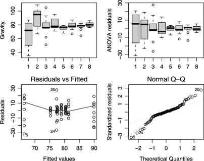
Figure 1: Gravity data and residual plots in Example 1 (sample sizes 8, 11, 9, 8, 8, 11, 13, and 13).

The decompositions by series for $\alpha=1$ and $\alpha=2$ are shown in Table 2. Note that when index $\alpha=2$ is applied, the DISCO decomposition is exactly equal to the ANOVA decomposition, also shown in Table 2. In fact, with our implementation as random permutation test, the $F_{2}$ test is actually a permutation test based on the ANOVA $F$ statistic. In this example 999 permutation replicates were used to estimate the $p$-values.

Table 2: Comparison of DISCO and ANOVA decompositions in Example 1

 

DISCO
  Distance Components: index 1.00
  Source            Df   Sum Dist  Mean Dist    F-ratio    p-value
  Between:
    Series           7  100.62287   14.37470      2.781      0.001
  Within            73  377.27836    5.16820

  Distance Components: index 2.00
  Source            Df   Sum Dist  Mean Dist    F-ratio    p-value
  Between:
    Series           7  2818.62413 402.66059      3.568      0.002
  Within            73  8239.37587 112.86816

ANOVA
  Analysis of Variance Table
  Response: Gravity
            Df Sum Sq Mean Sq F value  Pr(>F)
  Series     7 2818.6  402.7  3.5675 0.002357 [0.002 by perm. test]
  Residuals 73 8239.4  112.9

 

Residual plots from the fitted linear model (ANOVA) are shown in Figure 1, indicating that residuals have non-normal distribution and nonconstant variance. When we decompose residuals by Series using DISCO ($\alpha=1$) as shown in Table 3, the DISCO $F_{1}$ statistic is significant ($p$-value $<0.05$). We can conclude that the residuals do not arise from a common error distribution. (The ANOVA $F$ statistic is zero on residuals.)

Table 3: Distance Components of ANOVA residuals in Example 1

 

Distance Components: index  1.00
Source            Df   Sum Dist  Mean Dist   F-ratio   p-value
Between:
  Series           7   56.66334    8.09476     1.566     0.046
Within            73  377.27836    5.16820

 

The next example illustrates decomposition of residuals for a multivariate response.

Example 2 ((Iris data)).

Fisher’s (or Anderson’s) iris data set records four measurements (sepal length and width, petal length and width) for 50 flowers from each of three species of iris. The species are iris setosa, versicolor, and virginica. The data set is available in R (iris). The model is $Y\sim$ Species, where $Y$ is a four dimensional response corresponding to the four measurements of each iris. The DISCO $F_{1}$ and MANOVA Pillai–Bartlett $F$ test, implemented as permutation tests, each have $p$-value 0.001 based on 999 permutation replicates. The residuals from the fitted linear model are a $150\times 4$ data set.

Results of the multivariate analysis are shown in Table 4. From the DISCO decomposition of the residuals and test for equality of distributions of residuals ($p$-value $<0.04$), it appears that there are differences due to Species that are not explained by the linear component of the model.

Table 4: Analysis of iris data and residuals in Example 2

 

DISCO analysis of multivariate iris data:
    Distance Components: index   1.00
    Source           Df   Sum Dist   Mean Dist   F-ratio   p-value
    Between:
      Species         2  119.23731    59.61865   124.597     0.001
    Within          147   70.33848     0.47849

MANOVA analysis of multivariate iris data:
               Df Pillai approx F num Df den Df    Pr(>F)
   Species      2  1.192   53.466      8    290 < 2.2e-16 ***
   Residuals  147
   [permutation test p = 0.001]

DISCO analysis of residuals of linear model for iris data:
    Distance Components: index   1.00
    Source           Df   Sum Dist   Mean Dist   F-ratio   p-value
    Between:
      Species         2    1.69845     0.84923     1.775     0.039
    Within          147   70.33848     0.47849

 

5.3 Choosing the index $\alpha$

Choice of a test or a parameter for a test is a difficult question. Consider the similar situation one has with the choice of Cramér–von Mises tests, an infinite class of statistics that depend on the choice of weight function. For testing normality, for example, one can use the identity weight function (Cramér–von Mises test) or weight function $F(x)(1-F(x))$ (Anderson–Darling test) and both are good tests with somewhat different properties. Here we have a similar choice.

The simplest and most natural choice is $\alpha=1$ corresponding to Euclidean distance. It is natural because it is at the center of our interval for $\alpha$. Considering implementation for a univariate response, when $\alpha=1$ the Gini means can be linearized, which reduces the computational complexity from $O(N^{2})$ to $O(N\log(N))$.

For heavy-tailed distributions one may want to apply a small $\alpha$, which could be selected based on the data. As an example, consider the Pareto distribution with density $f(x)=k\sigma^{k}/x^{k+1}$, $x>\sigma$. In this case $E[X]$ exists only for $k>1$ and $\operatorname{Var}(X)$ is finite only for $k>2$. Note that $X^{\alpha}$ has a Pareto distribution for $\alpha>0$. If one is comparing claims data, which Pareto models tend to fit well, the tail index $k$ can be estimated by maximum likelihood to find a conservative choice of $\alpha$ such that the second moments of $X^{\alpha}$ exist. Heavy-tailed stable distributions such as Lévy distributions used in financial modeling suggest another situation where $\alpha<1$ may be recommended.

6 Simulation results

In this section we present the results of Monte Carlo studies to assess power of DISCO tests. In our simulations $R=199$ replicates are generated for each DISCO test decision.

Examples 3 and 4 compare DISCO with two parametric MANOVA tests based on Pillai (1955) and Wilks (1932) statistics (see, e.g., Anderson (1984, Chapter 8)). The Pillai–Bartlett test implemented in R is recommended by Hand and Taylor (1987).

Example 3.

The multivariate response is generated in a four group balanced design with common sample size $n=30$. The marginal distributions are independent with Student $t(4)$ distributions. Sample 1 is noncentral $t(4)$ with noncentrality parameter $\delta$. Samples 2–4 each have central $t(4)$ distributions. The index applied in the DISCO test is 1.0.

Results of several simulations are summarized in Figure 2(a) and (b) at significance level $0.10$. In Figure 2(a) the noncentrality parameter is on the horizontal axis and dimension is fixed at $p=10$. In Figure 2(b) the dimension is on the horizontal axis and $\delta=0.2$ is fixed. Each test achieves approximately the nominal significance level of $10\%$ under the null hypothesis [see Figure 2(a) at $\delta=0$]. Standard error of the estimate of power is at most 0.005, based on 10,000 tests.

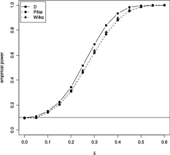
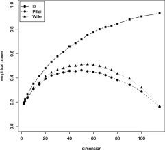
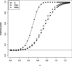
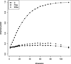
(a)	(b)

Figure 2: Monte Carlo results for Example 3: Empirical power of the DISCO and MANOVA tests against a t(4) alternative, four groups with $n=30$ per group, where (a) dimension $p=10$ and noncentrality parameter $\delta$ varies and (b) $p$ varies and $\delta=0.2$. Standard error of power estimate is at most 0.005.

Results displayed in Figure 2(a) and (b) suggest that the DISCO test is slightly more powerful than MANOVA tests against this alternative when $p=10$. As dimension increases, Figure 2(b) illustrates that the DISCO test is increasingly superior relative to MANOVA tests.

The MANOVA tests apply a transformation to obtain an approximate $F$ statistic. Although the data is non-normal, the MANOVA test statistics appear to be robust to non-normality in this example and exhibit good power when $p=10$. This simulation suggests that the transformation may not be applicable for test decisions when dimension is large relative to number of observations. For comparison with MANOVA tests, dimension is constrained by sample size. Note, however, that the DISCO test is applicable in arbitrary dimension regardless of sample size.

Example 4.

In this example we again consider a balanced design with four groups and $n=30$ observations per group. Groups 2–4 have i.i.d. marginal Gamma(shape${}={}$2, rate${}={}$0.1) distributions. Group 1 is alsoGamma(shape${}={}$2, rate${}={}$0.1), but with multiplicative errors distributed as Lognormal($\mu=0,\sigma$). Thus, the natural logarithm of the group 1 response has an additive normally distributed error with mean 0 and variance $\sigma^{2}$. The index applied is 1.0.

Results for significance level $10\%$ are summarized in Figures 3(a) and (b). Each test achieves approximately the nominal significance level of $10\%$ under the null hypothesis [see Figure 3(a) at $\sigma=0$]. Standard error of the estimate of power is at most 0.005, based on 10,000 tests.

(a)	(b)

Figure 3: Monte Carlo results for Example 4: Empirical power of the DISCO and MANOVA tests against a gamma(shape${}={}$2, rate${}={}$0.1) alternative, four groups with $n=30$ per group, where (a) dimension $p=10$ and $\sigma$ varies (b) $p$ varies and $\sigma=0.4$. Standard error of power estimate is at most 0.005.

In Figure 3(a) the parameter $\sigma$ is on the horizontal axis and dimension is fixed at $p=10$. Each test exhibits empirical power increasing with $\sigma$ in Figure 3(a), but the DISCO test is clearly more powerful than the MANOVA tests against this alternative. In Figure 3(b) the dimension is on the horizontal axis and $\sigma=0.4$ is fixed. This simulation reveals increasingly superior power performance of DISCO as dimension increases.

7 Summary

The distance components decomposition of total dispersion is analogous to the classical decomposition of variance, but generalizes the decomposition to a family of methods indexed by an exponent in $(0,2]$. The ANOVA and MANOVA methods are extended by choosing an index strictly less than 2, for which we obtain a statistically consistent test of the general hypothesis of equal distributions. DISCO tests can be applied in arbitrary dimension, which is not constrained by number of observations. The usual assumption of homogeneity of error variance is not required for DISCO tests, and the distribution of errors need not be specified except for the mild condition of finite variance. Moreover, the DISCO permutation test implementation is nonparametric and does not depend on the distributions of the sampled populations.

Appendix A

A.1 Proof of Proposition 1

The total sum of squared distances can be decomposed as

$$\sum\limits_{m=1}^{n_{2}}\sum\limits_{i=1}^{n_{1}}|a_{i}-b_{m}|^{2} = \sum\limits_{m=1}^{n_{2}}\sum\limits_{i=1}^{n_{1}}|a_{i}-\bar{a}+\bar{a}-b_{m}|^{2}$$

$$= \sum\limits_{m=1}^{n_{2}}[n_{1}\hat{\sigma}_{1}^{2}+n_{1}(\bar{a}-b_{m})^{2}]$$

$$= n_{1}n_{2}\hat{\sigma}_{1}^{2}+n_{1}\sum\limits_{m=1}^{n_{2}}(\bar{a}-\bar{b}+\bar{b}-b_{m})^{2}$$

$$= n_{1}n_{2}[\hat{\sigma}_{1}^{2}+\hat{\sigma}_{2}^{2}+(\bar{a}-\bar{b})^{2}],$$

where $\hat{\sigma}_{1}^{2}=(1/n_{1})\sum_{i=1}^{n_{1}}(a_{i}-\bar{a})^{2}$ and $\hat{\sigma}_{2}^{2}=(1/n_{2})\sum_{i=1}^{n_{2}}(b_{i}-\bar{b})^{2}$. Similarly,

$$\sum\limits_{m=1}^{n_{1}}\sum\limits_{i=1}^{n_{1}}|a_{i}-a_{m}|^{2}=2n_{1}^{2}\hat{\sigma}_{1}^{2}\quad\mbox{and}\quad\sum\limits_{m=1}^{n_{2}}\sum\limits_{i=1}^{n_{2}}|b_{i}-b_{m}|^{2}=2n_{2}^{2}\hat{\sigma}_{2}^{2},$$

so that

$$d_{2}(A,B) = \frac{n_{1}n_{2}}{n_{1}+n_{2}}\bigg{[}\frac{2}{n_{1}n_{2}}n_{1}n_{2}\bigl{(}\hat{\sigma}_{1}^{2}+\hat{\sigma}_{2}^{2}+(\bar{a}-\bar{b})^{2}\bigr{)}-\frac{1}{n_{1}^{2}}n_{1}^{2}\hat{\sigma}_{1}^{2}-\frac{1}{n_{2}^{2}}n_{2}^{2}\hat{\sigma}_{2}^{2}\bigg{]}$$

$$= \frac{2n_{1}n_{2}}{n_{1}+n_{2}}(\bar{a}-\bar{b})^{2}.$$

The well-known identity

$$n_{1}(\bar{a}-\bar{c})^{2}+n_{2}(\bar{b}-\bar{c})^{2}=\frac{n_{1}n_{2}}{n_{1}+n_{2}}(\bar{a}-\bar{b})^{2}$$ (16)

follows from $\bar{a}-\bar{c}=n_{2}(\bar{a}-\bar{b})/(n_{1}+n_{2})$ and $\bar{b}-\bar{c}=n_{1}(\bar{b}-\bar{a})/(n_{1}+n_{2})$. Hence, $d_{2}(A,B)=2n_{1}(\bar{a}-\bar{c})^{2}+2n_{2}(\bar{b}-\bar{c})^{2}=2\mathit{SST}$.

A.2 Proof of Theorem 2

One can obtain the DISCO decomposition by directly computing the difference between the total and within-sample dispersion. Given $p$-dimensional samples $A_{1},\dots,A_{K}$ with respective sample sizes $n_{1},\dots,n_{K}$ and $N=\sum_{j}n_{j}$, let $g_{jk}=g_{\alpha}(A_{j},A_{k})$ given by (3) and $G_{jk}=n_{j}n_{k}g_{jk}$, for $j,k=1,\dots,K$. Then for all $0<\alpha\leq 2$ and $p\geq 1$,

$$T_{\alpha}-W_{\alpha} = \frac{N}{2}g(A,A)-\frac{1}{2}\sum_{j}n_{j}g_{jj}$$

$$= \frac{N}{2}\biggl{(}\sum_{j<k}\frac{2}{N^{2}}G_{jk}+\sum_{j}\frac{1}{N^{2}}G_{jj}\biggr{)}-\frac{1}{2}\sum_{j}\frac{1}{n_{j}}G_{jj}$$

$$= \frac{1}{2N}\biggl{(}\sum_{j<k}2G_{jk}+\sum_{j}G_{jj}\biggr{)}-\frac{1}{2}\sum_{j}\frac{1}{n_{j}}G_{jj}$$

$$= \frac{1}{2N}\biggl{(}\sum_{j<k}n_{j}n_{k}(2g_{jk}-g_{jj}-g_{kk})+\sum_{j<k}n_{j}n_{k}(g_{jj}+g_{kk})\biggr{)}$$

$${}+\frac{1}{2N}\sum_{j}n_{j}^{2}g_{jj}-\frac{1}{2}\sum_{j}n_{j}g_{jj}$$

$$= \sum_{j<k}\frac{n_{j}+n_{k}}{2N}\biggl{(}\frac{n_{j}n_{k}}{n_{j}+n_{k}}\biggr{)}(2g_{jk}-g_{jj}-g_{kk})+\frac{1}{2N}\sum_{j<k}n_{k}(n_{j}g_{jj})$$

$${}+\frac{1}{2N}\sum_{j<k}n_{j}(n_{k}g_{kk})+\frac{1}{2N}\sum_{j}n_{j}^{2}g_{jj}-\frac{1}{2}\sum_{j}n_{j}g_{jj}.$$

After simplification we have

$$T_{\alpha}-W_{\alpha} = \sum_{j<k}\frac{n_{j}+n_{k}}{2N}\biggl{(}\frac{n_{j}n_{k}}{n_{j}+n_{k}}\biggr{)}(2g_{jk}-g_{jj}-g_{kk})$$

$${}+\frac{1}{2N}\sum_{k}\sum_{j}n_{k}(n_{j}g_{jj})-\frac{1}{2}\sum_{j}n_{j}g_{jj}$$

$$= \sum_{j<k}\frac{n_{j}+n_{k}}{2N}\biggl{(}\frac{n_{j}n_{k}}{n_{j}+n_{k}}\biggr{)}(2g_{jk}-g_{jj}-g_{kk})$$

$${}+\frac{N}{2N}\sum_{j}n_{j}g_{jj}-\frac{1}{2}\sum_{j}n_{j}g_{jj}$$

$$= \sum_{j<k}\frac{n_{j}+n_{k}}{2N}\biggl{(}\frac{n_{j}n_{k}}{n_{j}+n_{k}}\biggr{)}(2g_{jk}-g_{jj}-g_{kk})=B_{\alpha}.$$