An electron jet pump: The Venturi effect of a Fermi liquid

Abstract

A three-terminal device based upon a two-dimensional electron system is investigated in the regime of non-equilibrium transport. Excited electrons scatter with the cold Fermi sea and transfer energy and momentum to other electrons. A geometry analogous to a water jet pump is used to create a jet pump for electrons. Because of its phenomenological similarity we name the observed behavior the “electronic Venturi effect”.

I introduction

The Venturi effect in hydrodynamics describes the relation between the pressure of an inviscid fluid and the cross-section of the tubing it flows through, as a reduced cross-section leads to reduced pressure. One of the more famous applications of this phenomenon is the water jet pump indroduced by Bunsen in 1869 Bunsen (1869) in which the decrease of fluid pressure in a constriction is used for evacuating a side port. Beyond the bottleneck, the fluid reaches a wider collector tube and decelerates. Here we present a similar system, an “electron jet pump,” built from a degenerate two-dimensional electron system, a Fermi liquid. “Hydrodynamic” effects in Fermi liquids have been studied theoretically Govorov and Heremans (2004) and experimentallyDyakonov and Shur (1993), however, “hydrodynamic” has been used in different ways. While e. g., Ref. Dyakonov and Shur, 1993 describes a system governed by a set of equations essentially identical to those describing hydrodynamics and Ref. Gardner, 1994 extends these equations to a quantum-mechanical regime, Ref. Govorov and Heremans, 2004 along with the experiments presented here use hydrodynamics as a qualitative analogy since the results are very similar from a phenomenological point of view. The electronic analogy of the Venturi effect has been introduced in Ref. Taubert et al., 2010; other experiments describing related physics but, in part, based upon different effects have been performed since the 1990s.Brill and Heiblum (1994); Kaya and Eberl (2007)

II device and setup

Fig. 1(a)

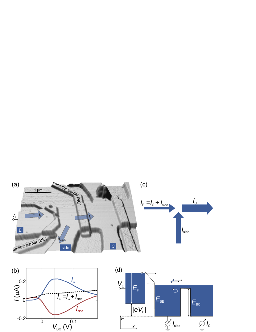
Figure 1: (Color online) (a) Atomic force micrograph of the sample. Elevated areas represent metal gates fabricated on top of a hall bar defined by wet etching. Definition of positive current directions (direction of electron flow) is marked by arrows. (b) Three currents defined in (a) as a function of voltage applied to gate BC for $V_{\text{BE}}=$-0.925\text{\,}\mathrm{V}$$, $V_{\text{E}}=$-155.3\text{\,}\mathrm{mV}$$ (c) Diagram of arrows showing the actual current directions, at position marked in (b) by a vertical line, with the arrow width resembling the magnitude of current, and (d) model of electronic Venturi effect (see main text).

shows an atomic force micrograph of the device used to demonstrate the electronic Venturi effect. It has been fabricated from a GaAs/AlGaAs heterostructure containing a two-dimensional electron system (2DES) $90\text{\,}\mathrm{nm}$ below the surface. The 2DES has a mobility of $\mu=1.4\times 10^{6}\,\text{cm}^{2}/\text{Vs}$ (at $T\approx 1\,\text{K}$) and a Fermi energy of $E_{\text{F}}=9.7\,\text{meV}$ (carrier density $n_{s}=2.7\times 10^{15}\,\text{m}^{-2}$). The elastic mean-free path $l_{\text{m}}\simeq 12\;\mu\text{m}$ is much larger than the sample dimensions. All measurements presented here have been performed in a ³He cryostat at a bath temperature of $260\text{\,}\mathrm{mK}$, but similar results have been obtained in a temperature range of $20\,\text{mK}\leq T_{\text{bath}}\leq 20\,$K in several comparable samples.

A hall-bar-like structure created by wet etching defines the general layout of the device with a central area with several terminals connected to ohmic contacts (not visible). Three of them are used in the experiments shown here, namely the emitter “E”, “side” contact, and collector “C”. Additionally, metallic gates [elevated in Fig. 1(a)] are used to electrostatically define the barriers. A quantum point contact, called the “BE” (emitter barrier), and a broad collector barrier “BC” are used for demonstrating the electronic Venturi effect; the device contains more gates, though. All measurements presented here have been performed with the QPC as emitter, but using a broad barrier as “BE” produces very similar results. The special nature of a QPC is, therefore, not crucial. The terminal in the top right corner of Fig. 1(a) did not carry current, which might be related to the contamination visible in the micrograph.

III electron jet pump

A bias voltage, $V_{\text{E}}$, is applied to the emitter contact while “side” and “C” are grounded via low-noise current amplifiers. At the emitter, a current, $I_{\text{E}}$, flows which we define to be positive if electrons are injected into the device ($V_{\text{E}}<0$). In a network of ohmic resistors, the electrons would be expected to leave the device at the two contacts “side” and “C”; we thus define the resulting currents, $I_{\text{side}}{}$ and $I_{\text{C}}$, to be positive in such an ohmic situation. For the definitions applied here, Kirchhoff’s current law therefore reads, $I_{\text{E}}=I_{\text{C}}+I_{\text{side}}{}$ [also compare arrows in Fig. 1(a)].

Fig. 1(b) shows the simultaneously measured dc currents, $I_{\text{C}}$ and $I_{\text{side}}{}$, along with the derived quantity, $I_{\text{E}}$, as a function of $V_{\text{BC}}$, which is the voltage applied to the collector barrier. In most of the plot, non-ohmic behavior is observed as $I_{\text{C}}$ exceeds $I_{\text{E}}$, equivalent to a negative side current. This behavior is visualized in Fig. 1(c) which shows three arrows resembling the currents for a situation marked in Fig. 1(b) by a vertical line. The width of the arrows stands for the magnitude of the respective currents. As more electrons leave the device at “C” than are injected at “E”, this effect can be viewed as amplification of the injected current. Alternatively, and concurrent with the hydrodynamic analogy, it can be interpreted as jet pump behavior, as electrons are drawn into the device at the side port.

The observed effect can be understood as follows. Due to the voltage drop of $V_{\text{E}}$ across the emitter barrier BE, which is close to pinch-off, electrons are injected into the central region of the device with a kinetic energy of approximately $\left|eV_{\text{E}}+E_{\text{F}}\right|$, which is $163\text{\,}\mathrm{m}\evolt$ in the case of Fig. 1(b). Electrons with such an energy scatter rather efficiently with the cold Fermi sea (the energy dependence of electron-electron scattering will be discussed in section V), and thereby excite electron-hole pairs (in this case, “hole” means a missing electron in the Fermi sea, not a valence band hole). If the collector barrier has a suitable height, as in the center of Fig. 1(b), it will separate excited electrons from the Fermi sea holes. While the electrons pass the barrier, the positively charged holes are trapped between BE and BC. Without a connection to the environment, a positive charge would accumulate hereTaubert et al. (2010), but since the side contact is grounded and therefore provides a reservoir of charge carriers, electrons are drawn from this contact into the device. The jet pump analogy is therefore especially appealing as it incorporates the attractive force exerted on the “fluid“ in the side port.

IV Influence of the collector barrier

IV.1 Calibration of collector barrier height

The collector barrier BC is first and foremost characterized by the applied gate voltage, $V_{\text{BC}}$, but its height, $E_{\text{BC}}$, compared to the Fermi energy would be more useful. We have determined the actual height of a barrier in units of energy (for barriers below the Fermi energy) by measuring the reflection of Landau levels at the barrier in a perpendicular magnetic fieldKomiyama et al. (1989); Haug et al. (1988) as in Refs. Taubert et al., 2010 and Schinner et al., 2009.

In contrast to the experiments described in the rest of the article, these calibration measurements are performed in the linear-response regime using the lock-in technique with $V_{E,\text{rms}}=75\;\mu\text{V}$ at $18.4\text{\,}\mathrm{Hz}$ ($V_{E,\text{rms}}$ is kept small to minimize distortion of the barrier shape due to a voltage drop across the barrier). Fig. 2(a)

Figure 2: (Color online) (a) Pinch-off curves of barrier BC in a perpendicular magnetic field at integer filling factors $\nu$. Reflection of landau levels at BC creates plateaus in the curves (see sketch); crosses mark data points used for the calibration. (b) Points: allocated energies as a function of gate voltages at plateau centers extracted from the set of curves shown in (a) and corresponding energies, “$B=0$” denotes additional calibration for zero field (see text); line: fit of all data points, used for determining conversion between $V_{\text{BC}}$ and $E_{\text{BC}}$.

plots the ac collector current, $I_{\text{C}}$, in a two-terminal measurement (side contact floating) as a function of the voltage, $V_{\text{BC}}$, which controls the barrier height $E_{\text{BC}}$. Pinch-off curves for different magnetic fields with integer bulk filling factors $6\leq\nu\leq 14$ in the undisturbed 2DES are shown.

The inset of Fig. 2(a) demonstrates how the reflection of Landau levels can be used in this setup to extract information about the barrier height (sketch for filling factor $\nu=6$): At the position of the barrier, the number of occupied Landau levels is reduced. The higher the barrier, the more Landau levels are pushed above the Fermi edge and therefore do not contribute to the transmission. As long as the number of Landau levels between the top of the barrier and the Fermi energy does not change, the transmission should stay constant, and a plateau in the current is expected. At the center of the plateau we have $E_{\text{F}}-E_{\text{BC}}=k\;\hbar\omega_{c}$ with $k\in{1,2,\dots,\nu/2}$. The plateau positions in $V_{\text{BC}}$, and the respective value of $k$, can be determined for several bulk filling factors $\nu$ as shown in Fig. 2(b). We estimate the error of the plateau position to be about $5\text{\,}\mathrm{mV}$ [as marked in Fig. 2(b)]. The energy values are much more accurate since their main error source is an inaccuracy in the magnetic field value, e. g., due to ferromagnetic material. Shubnikov-de Haas oscillations periodic in $1/B$ observed in the same measurement run suggest a neglibile error in $B$ and therefore in energy. The pinch-off curve for $B=0$ yields one additional data point, the gate voltage corresponding to $E_{\text{BC}}=E_{\text{F}}$ [marked by “$B=0$“ in Fig. 2(b)] at which current starts to flow across the barrier in a two-terminal setup. A linear fit to all datapoints yields the relation $E_{\text{BC}}=-0.025\;eV_{\text{BC}}-$8.4\text{\,}\mathrm{m}\evolt$$ as our final barrier calibration.

The barriers used in the experiments presented here turned out to be sufficiently stable over a long period of time so that it was enough to perform the calibration once per barrier. The only exception was a sudden dramatic shift of the pinch-off curves of a single barrier (in the order of $300\text{\,}\mathrm{mV}$ toward more positive voltages). Those changes were irreversible, seemingly not caused by external influences, and only happened once per barrier. Since they were easy to detect, they did not consitute a serious problem, only the calibration had to be repeated. The measurements shown in Figs. 1(b), 3, and 4 have been performed after the barrier had changed, hence $V_{\text{BC}}>0$. For this set of data, the calibration relation, $E_{\text{BC}}=-0.026\;eV_{\text{BC}}-$0.35\text{\,}\mathrm{m}\evolt$$ was obtained.

IV.2 Tuning for amplification

Fig. 3(a)–(c)

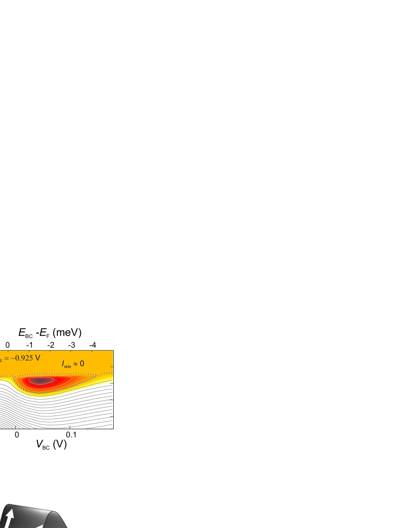
Figure 3: (Color online) Side current as a function of collector barrier voltage $V_{\text{BC}}$ and bias voltage $V_{\text{E}}$. Collector barrier height calculated from $V_{\text{BC}}$ as shown in section IV.1 is depicted on upper axis. Contour lines spaced by $70\text{\,}\mathrm{nA}$ are drawn in black for $I_{\text{side}}{}>0$, in white for $I_{\text{side}}{}<0$, and dashed lines for $I_{\text{side}}{}\approx 0$. Emitter barrier voltage $V_{\text{BE}}$ is (a) $-0.725\text{\,}\mathrm{V}$, (b) $-0.925\text{\,}\mathrm{V}$, and (c) $-1.125\text{\,}\mathrm{V}$; (d) sketch to demonstrate 2D model of barrier height influence (see main text for details).

show measurements of $I_{\text{side}}{}$ as a function of collector barrier height (on the top axis; the corresponding gate voltage $V_{\text{BC}}$ is shown on the bottom axis) and bias voltage $V_{\text{E}}$. In the upper part of the graphs, $I_{\text{side}}{}\approx 0$, since here the emitter is closed. The current starts to flow into the device at a threshold bias, e. g., $V_{\text{E}}^{\text{th}}\approx$-150\text{\,}\mathrm{mV}$$ for Fig. 3(b). Upon crossing the threshold $I_{\text{side}}{}$ immediately becomes negative in the central area of the plots (framed by a dashed line marking $I_{\text{side}}{}=0$), corresponding to amplification. For larger bias voltages, the side current changes sign and quickly increases ($I_{\text{side}}{}<0$). The latter effect is actually related to an increase in the total current flowing through the device and has been discussed in detail in Ref. Taubert et al., 2010.

From Figs. 3(a) to 3(c), $V_{\text{BE}}$ is made more negative, which has several implications. One consequence is a shift in the threshold bias $V_{\text{E}}^{\text{th}}$ to larger energies since the emitter is more closed for more negative $V_{\text{BE}}$. In addition, the area of $I_{\text{side}}{}<0$ and the magnitude of $I_{\text{side}}{}$ depend on $V_{\text{E}}^{\text{th}}(V_{\text{BE}})$, with the largest effect visible in Fig. 3(b). More details, including a discussion of the area showing $I_{\text{side}}{}\approx 0$ at large $V_{\text{E}}$ [Fig. 3(c)], will be given in section V.

IV.3 Model

Fig. 3 demonstrates that the electron jet pump behavior depends strongly upon the collector barrier height. Strikingly, $I_{\text{side}}{}<0$ is exclusively found when BC is below the Fermi energy ($E_{\text{BC}}<E_{\text{F}}$). This excludes heating as the reason of the observed effect since in this case the maximum effect would be expected for $E_{\text{BC}}>E_{\text{F}}$. In a naïve one-dimensional model based on non-equilibrium electron-electron scattering (Sec. III), the BC exactly at the Fermi energy would result in the best charge separation since then all excited electrons (above $E_{\text{F}}$) would pass the barrier while all holes (below $E_{\text{F}}$) would be reflected. Maximal amplification would therefore be expected at $E_{\text{BC}}=E_{\text{F}}$, and the area of $I_{\text{side}}{}<0$ would roughly be centered around this point.

The device studied here is two-dimensional (2D) in nature, and in 2D the very simple model has to be modified. In 1D, it was sufficient to look at the total kinetic energy of an electron to determine whether it will pass the barrier or it will be reflected. In 2D, only the forward momentum component, $p_{\perp}$, perpendicular to the barrier is significant. A charge carrier can only cross the barrier if $p_{\perp}^{2}/2m>E_{\text{BC}}$ is fulfilled, thus passing the barrier is harder for particles not perpendicularly hitting it. A simple classical analogy to this situations is depicted in Fig. 3(d), showing two balls rolling towards a hill with the same velocity but at different angles. The ball hitting the barrier perpendicularly will pass more easily than the one moving at an angle. If one now considers a large amount of charge carriers with a distribution of angles in 2D, less carriers will cross a barrier of the same height as compared to the 1D case. In other words, the barrier has to be lowered, compared to 1D, to reach a comparable amount of passing charge carriers. This explains why the jet pump effect is shifted to lower barrier heights ($E_{\text{BC}}<E_{\text{F}}$) than predicted by the simple 1D model.

V Electron-electron scattering length

In the $I_{\text{side}}{}$ measurements presented up to now, the collector barrier ($V_{\text{BC}}$) was varied while the emitter barrier ($V_{\text{BE}}$) was kept constant. It is also instructive to analyze data for a fixed $V_{\text{BC}}$ while $V_{\text{BE}}$ is varied. An example of such a measurement is shown in Fig. 4(a).

Figure 4: (Color online) (a) $I_{\text{side}}{}$ as a function of $V_{\text{BE}}$ and $V_{\text{E}}$ measured for dissipated powers $\left|V_{\text{E}}\times I_{\text{E}}\right|\leq 700\,$nW. No data exist for higher powers (lower right corner) and for the upper left corner; here the emitter QPC is closed and all currents vanish. (b) Same data as in (a), plotted as a function of injected current, $I_{\text{E}}$; contour lines are spaced by $70\text{\,}\mathrm{nA}$, $I_{\text{side}}{}\approx 0$ is marked by a dashed line. (c) Vertical slice of Fig. 4(a) at $I_{\text{E}}=0.15\;\mu\text{A}$; (d) numerical calculations of electron-electron scattering length, $l_{\text{ee}}$, as a function of excess kinetic energy $|eV_{\text{E}}|\simeq E_{\text{kin}}-E_{\text{F}}$ at $T=0$; the dashed line marks sample dimensions.

The threshold of nonvanishing current through the device is visible along a roughly diagonal line. Above that, in the upper left corner, all currents are zero; therefore, most of this area has not been mapped out in detail. The lower right corner also contains no measured data points, since here, at rather open emitter and large negative bias, the power dissipated in the device would be very high. For the actual measurement, power was therefore limited to $\left|V_{\text{E}}\times I_{\text{E}}\right|\leq 700\,$nW.

In an approximately diagonal stripe tapered at both ends, $I_{\text{side}}{}<0$ is visible (in addition, in the upper right corner a region with $I_{\text{side}}{}<0$ due to ohmic behavior is observed at $V_{\text{E}}>0$). The data show the same general behavior already visible in Figs. 3(a)–3(c). It is far easier to analyze another representation of the data, depicted in Fig. 4(b), which shows $I_{\text{side}}{}$ as a function of $V_{\text{E}}$ and the total current $I_{\text{E}}=I_{\text{C}}+I_{\text{side}}{}$ ($I_{\text{side}}{}$ and $I_{\text{C}}$ were measured). Below the straight solid line the resistance of the emitter is $\left|V_{\text{E}}\right|/I_{\text{E}}>$100\text{\,}\mathrm{k\SIUnitSymbolOhm}$$ (contact resistances are much smaller). The emitter is thus almost pinched off, and we can assume that all electrons contributing to $I_{\text{E}}$ are injected at BE with an energy close to $\left|eV_{\text{E}}\right|$. Vertical (horizontal) slices of Fig. 4(b) therefore show $I_{\text{side}}{}$ as a function of energy (power) at constant $I_{\text{E}}$ (energy per electron) (see Ref. Taubert et al., 2010). Here we concentrate on the energy dependence.

Fig. 4(c) shows a slice of Fig. 4(b) at constant total current, allowing one to analyze the dependence of $I_{\text{side}}{}$ upon excess kinetic energy $\left|eV_{\text{E}}\right|$ right at the maximum of the observed effect (most negative $I_{\text{side}}{}$). For very small $\left|V_{\text{E}}\right|$, $I_{\text{side}}{}$ is positive, then rapidly decreases to reach its minimum value at an energy of $\left|eV_{\text{E}}\right|\approx$150\text{\,}\mathrm{m}\evolt$$. For larger energies $I_{\text{side}}{}$ again increases and takes positive values. However, for $\left|eV_{\text{E}}\right|>$300\text{\,}\mathrm{m}\evolt$$ $I_{\text{side}}{}$ decreases once more, and then vanished in the high-energy limit. The latter phenomenon is also visible in Fig. 4(b) as an extended area of $I_{\text{side}}{}\approx 0$ as well as in Fig. 3(c).

The behavior of $I_{\text{side}}{}$ as a function of $\left|eV_{\text{E}}\right|$ is closely related to the energy dependence of the electron-electron scattering length, $l_{\text{ee}}$. Predictions of $l_{\text{ee}}$ near the linear response regime have been made before,Chaplik (1971); Giuliani and Quinn (1982) but to describe scattering of a single electron with a 2DES, at a kinetic energy greatly exceeding $E_{\text{F}}$, an extension of those earlier models is necessary. We have performed numerical calculations for $T=0$ based on the random phase approximation to determine $l_{\text{ee}}$ as a function of excess kinetic energy for the whole energy range accessible in the experiments presented here. The result is shown in Fig. 4(d). As the kinetic energy $E_{\text{kin}}=\left|eV_{\text{E}}\right|+E_{\text{F}}$ exceeds $E_{\text{F}}$, electron-hole excitations cause a rapid decrease of $l_{\text{ee}}$ as a function of $\left|eV_{\text{E}}\right|$ [$l_{\text{ee}}\propto 1/((p-p_{\text{F}})\ln(\left|p-p_{\text{F}}\right|))$]. The subsequent increase of $l_{\text{ee}}\propto\left|eV_{\text{E}}\right|$ toward high kinetic energies ($E_{\text{kin}}\gg E_{\text{F}}$) is caused by a decreased interaction time in combination with a suppressed plasmon radiation. This result compairs fairly well with its three-dimensional (3D) counterpartPines and Noizières (1966). A major reason for this similarity is that plasmon radiation in 3D is also suppressed below a threshold energy, although with a different origin compared to 2DGiuliani and Quinn (1982).

The behavior of $l_{\text{ee}}$ can be mapped onto the measured energy dependence of $I_{\text{side}}{}$ [Fig. 4(c)] if the sample geometry is taken into account. A dashed horizontal line in Fig. 4(d) marks $840\text{\,}\mathrm{nm}$, the distance between BE and BC. Electrons injected with energies corresponding to a $l_{\text{ee}}$ smaller than this distance have a high probability of scattering between BE and BC, thereby contributing to the jet pump effect by creating electron-hole pairs in the central region. Energies corresponding to a small $l_{\text{ee}}$ and a positive slope of the curve in Fig. 4(d) are even more favorable since hot electrons always lose energy in scattering with the Fermi sea, thus after one scattering event the scattering length can be reduced even further. This is likely to result in multiple scattering processes which produce many electron-hole pairs, leading to a very negative $I_{\text{side}}{}$. As $\left|V_{\text{E}}\right|$ is increased further, $l_{\text{ee}}$ exceeds the sample dimensions, and scattering events tend to happen beyond BC. In an intermediate regime, scattering beyond BC, but still close to the barrier, may lead to scattered electrons traveling back accross BC and into the side contact which causes a positive $I_{\text{side}}{}$, which is visible in Fig. 4(c) as a local maximum at around $320\text{\,}\mathrm{m}\evolt$. At the highest energies studied here, $I_{\text{side}}{}\approx 0$, which is consistent with the very large value of $l_{\text{ee}}$ predicted by our numerics. Here, electrons move ballistically through the sample and scatter only very far away from BC so that no electron-hole separation occurs. No charge carriers reach the side contact, and $I_{\text{side}}{}=0$.

VI Influence of magnetic field

Scattering lengths are expected to change considerably if external parameters are varied. Here the influence of a magnetic field perpendicular to the two-dimensional electron system ist studied. Figures 5(a)–5(c)

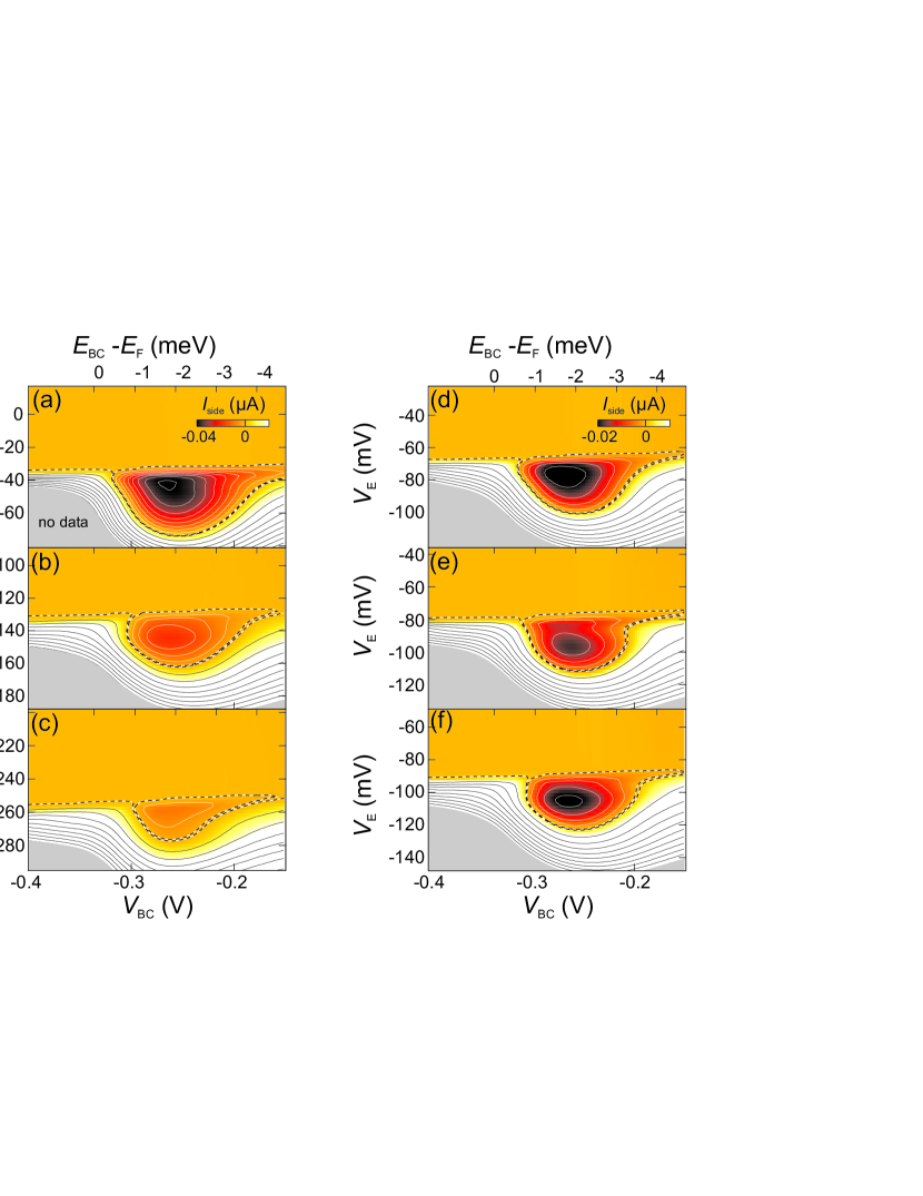
Figure 5: (Color online) Measurements similar to those in Fig. 3 with a magnetic field of $5.2\text{\,}\mathrm{T}$ perpendicularly applied. Contour lines spaced by $5\text{\,}\mathrm{nA}$ for $I_{\text{side}}{}<0$ (white) and $10\text{\,}\mathrm{nA}$ for $I_{\text{side}}{}>0$ (black). Emitter barrier voltage $V_{\text{BE}}=$-0.675\text{\,}\mathrm{V}$$ in (a), $-0.875\text{\,}\mathrm{V}$ in (b), $-1.075\text{\,}\mathrm{V}$ in (c), $-0.750\text{\,}\mathrm{V}$ in (d), $-0.775\text{\,}\mathrm{V}$ in (e), and $-0.800\text{\,}\mathrm{V}$ in (f).

show measurements similar to those presented in Fig. 3(a)–(c), with an additional perpendicular magnetic field of $B=$5.2\text{\,}\mathrm{T}$$. The field direction is ”upwards,” i. e., electrons injected into the central part of the sample are guided to their left, away from the side contact. Data with and without the magnetic field look rather similar. However, the magnitude of the negative side current is smaller by roughly a factor of 5 (note different color scale compared to Fig. 3) while the overall current passing through the device is virtually unchanged. A regime of $I_{\text{side}}{}\approx 0$ has been observed at high energies as in the case of $B=0$, but it is not included in the set of data shown here.

Figures 5(d)–5(f) show a series of measurements at more closely spaced emitter barrier voltages of $V_{\text{BE}}=$-0.750\text{\,}\mathrm{V}$$ in (d), $-0.775\text{\,}\mathrm{V}$ in (e), and $-0.800\text{\,}\mathrm{V}$ in (f). The color scale is different from Fig. 5(a)–5(c) to show the detailed structure of the data. Here a nonmonotonic dependence on $V_{\text{BE}}$ not visible in the overview series shown in Figs. 5(a)–5(c) is observed. Here, $I_{\text{side}}{}$ is less negative in Fig. 5(e) compared to Fig. 5(d) and 5(f), and shows a peculiar structure inside the area of $I_{\text{side}}{}<0$: two minima with a lighter stripe in between. These substructures are related to the emission of optical phonons which lead to a periodic reduction of negative side current as a function of kinetic energy; the period being $36\text{\,}\mathrm{m}\evolt$, which is the energy of optical phonons in GaAsHickmott et al. (1984). Traces of optical phonon emission are already visible in the zero-field data presented in Fig. 4(b) and 4(c) at low energies as oscillations of $I_{\text{side}}{}(V_{\text{E}})$. The emission of optical phonons and its relation to the electron jet pump is discussed in detail in Ref. TODO onlinecite

VII Conclusion

We have studied the electronic Venturi effect in a relatively simple device containing three current-carrying contacts and two barriers. Here the influence of the second, “collector,” barrier has been investigated in detail, since it is vitally important to create an electron jet pump. Such a device might have an application in amplifying small currents or charges down to single electrons.