On the origin of the Type ii spicules - dynamic 3D MHD simulations

Abstract

Recent high temporal and spatial resolution observations of the chromosphere have forced the definition of a new type of spicule, “type ii’s”, that are characterized by rising rapidly, having short lives, and by fading away at the end of their lifetimes. Here, we report on features found in realistic 3D simulations of the outer solar atmosphere that resemble the observed type ii spicules. These features evolve naturally from the simulations as a consequence of the magnetohydrodynamical evolution of the model atmosphere. The simulations span from the upper layer of the convection zone to the lower corona and include the emergence of horizontal magnetic flux. The state-of-art Oslo Staggered Code (OSC) is used to solve the full MHD equations with non-grey and non-LTE radiative transfer and thermal conduction along the magnetic field lines. We describe in detail the physics involved in a process which we consider a possible candidate as a driver mechanism to produce type ii spicules. The modeled spicule is composed of material rapidly ejected from the chromosphere that rises into the corona while being heated. Its source lies in a region with large field gradients and intense electric currents, which lead to a strong Lorentz force that squeezes the chromospheric material, resulting in a vertical pressure gradient that propels the spicule along the magnetic field, as well as Joule heating, which heats the the jet material, forcing it to fade.

1 Introduction

The upper solar chromosphere is filled with highly dynamic jets. These jet phenomena go under several names, depending on the location they are observed at and on their physical characteristics. Examples are dynamic fibrils found in active regions on the disk, mottles found in the quiet sun on the disk, and spicules at the limb (Beckers, 1968; Suematsu et al., 1995; Hansteen et al., 2006; De Pontieu et al., 2007c; Rouppe van der Voort et al., 2007). Spicules at the limb are observed in the H$\alpha$ line and in other chromospheric lines such as the Ca ii H & K lines. With the large improvement in spatio-temporal stability and resolution given by the Hinode satellite (Kosugi et al., 2007), and with the Swedish 1-m Solar Telescope (SST) (Scharmer et al., 2008), it has been discovered that spicules come in at least two clearly identified physical types with different dynamics and timescales (De Pontieu et al., 2007b).

The so-called type i spicules occur on time-scales of 3-10 minutes, develop speeds of 10-30 km s^-1, reach heights of 2-9 Mm (Beckers, 1968; Suematsu et al., 1995), and typically involve upward motion followed by downward motion. Shibata & Suematsu (1982); Shibata et al. (1982) studied in detail the propagating shocks in simplified 1D models where they increased the temperature at specific heights and the velocities are not larger than the sound speed. The position of the top of the spicule follows a parabolic profile in time, which is indicative of an upwardly propagating shock passing through the upper chromosphere and transition region towards the corona as modeled and described by Hansteen et al. (2006), De Pontieu et al. (2007a), Heggland et al. (2007), and in 3D by Martínez-Sykora et al. (2009a). The latter authors described how the spicule-driving shocks can be generated by a variety of processes, such as collapsing granules, overshooting p-modes, dissipation of magnetic energy in the photosphere and lower-chromosphere, or any other sufficiently energetic phenomenon in the upper photosphere or chromosphere. Matsumoto & Shibata (2010) claim that spicules can be driven by resonant Alfvén waves, generated in the photosphere and confined in a cavity between the photosphere and transition region.

Type ii spicules, observed in Ca ii and H$\alpha$, have shorter lifetimes than type i spicules, typically less than 100 seconds, are more violent, with upward velocities of the order of 50-100 km s^-1, and reach somewhat greater heights. They usually exhibit only upward motion (De Pontieu et al., 2007c), followed by a rapid fading in chromospheric lines without any observed downfall. Spicules of type ii seen in the Ca ii band of Hinode show fading on time-scales of the order of a few tens of seconds (De Pontieu et al., 2007b). The disk counterparts to this class of spicules are denominated “Rapid Blue-shifted Events” (RBEs) (Langangen et al., 2008; Rouppe van der Voort et al., 2009). These show strong Doppler blue shifts in lines formed in the middle to upper chromosphere. De Pontieu et al. (2009) linked the RBEs with asymmetries in transition region and coronal spectral line profiles. The increase in line broadening during the lifetime of RBE suggest that they are heated to at least transition region temperatures (De Pontieu et al., 2007b; Rouppe van der Voort et al., 2009). Another intriguing observation is that type ii spicules often also appear in regions that seem unipolar (McIntosh & De Pontieu, 2009).

The latter observation complicates explanations of the type ii phenomena by magnetic reconnection, which seems a likely candidate for other types of coronal jets. For example, the pioneering 2D simulations done by Yokoyama & Shibata (1995, 1996), or more recent simulations done by Nishizuka et al. (2008) shows that emerging magnetic flux reconnects with an open ambient magnetic field forming a large angle to the emerging field. Such reconnection produces strong velocities and a jet, with a large energy release. 3D experiments of jet formation in a horizontally magnetized atmosphere as consequence of a reconnection trigger, where the flux emergence is a prime candidate have been done by Archontis et al. (2005); Galsgaard et al. (2007). Moreno-Insertis et al. (2008) expanded the Yokoyama & Shibata (1995) model to 3D, where the ambient field is open and connects into the corona.

In this paper discussion is confined to type ii spicules, since 3D models of the first type have been described previously by Martínez-Sykora et al. (2009a). We analyze a jet-like feature that we find in a realistic 3D-MHD simulation that shares many of the characteristics of the observed type ii spicules. The simulation includes non-grey and non-LTE radiative transfer with scattering, and thermal conduction along the magnetic field lines. The model spans the upper layers of the convection zone to the lower corona. In § 2 the numerical methods are briefly described, while the initial model and boundary conditions employed are described in § 3. In § 4.1, we describe the structure of the spicule-like jet which is found in the model. We succeed in isolating the mechanism far enough to find the initial configuration in the photosphere that starts the chain of events leading to the jet (see § 4.2). The physics, dynamics, and the detailed evolution of the formation mechanism are described in § 4.3. The fading of the jet from the chromosphere is discussed in § 4.4. In § 4.5 the mass and enthalpy flux associated with the jet is analyzed. Conclusions are presented in § 5.

2 Equations and Numerical Method

The MHD equations are solved in our physical domain using the Oslo Stagger Code (OSC). The numerical methods have been described in detail in Dorch & Nordlund (1998); Mackay & Galsgaard (2001); Martínez-Sykora et al. (2008, 2009b). In short, the code functions as follows: A sixth order accurate method is used for determining the partial spatial derivatives. In instances where variables are needed at positions other than their defined grid positions a fifth order interpolation scheme is used. The equations are stepped forward in time using the explicit third order predictor-corrector procedure described by Hyman et al. (1979), modified for variable length time steps. In order to suppress numerical noise, high-order artificial diffusion is added both in the forms of a viscosity and in the form of a magnetic diffusivity.

The radiative flux divergence from the photosphere and lower chromosphere is obtained by angle and wavelength integration of the transport equation assuming isotropic opacities and emissivities. The transport equation assumes that opacities are in LTE using four group mean opacities to cover the entire spectrum (Nordlund, 1982). This is done by formulating the transfer equation for each of the four bins, calculating a mean source function in each bin. These source functions contain an approximate coherent scattering term and an exact contribution from thermal emissivity. The resulting 3D scattering problems are solved by iteration, based on one-ray approximation in the angle integral for the mean intensity, a method developed by Skartlien (2000).

In the mid and upper chromosphere the OSC code includes non-LTE radiative losses from tabulated hydrogen continua, hydrogen lines, and lines from singly ionized calcium as functions of temperature and column mass. These radiative losses depend of the computed non-LTE escape probability as a function of column mass and are based on a 1D dynamical chromospheric model in which the radiative losses are computed in detail (Carlsson & Stein 1992, 1994, 1997, 2002).

For the upper chromosphere and corona we assume optically thin radiative losses. The optically thin radiative loss function based on the coronal approximation and atomic data collected in the HAO spectral diagnostics package (Judge & Meisner, 1994) is based on the elements hydrogen, helium, carbon, oxygen, neon and iron.

The model includes thermal conduction along the magnetic field. The conductive term is split from the energy equation and is discretized using the Crank-Nicholson method. The resulting operator is implicit and is solved using a multi-grid solver (see Martínez-Sykora et al., 2008).

The energy dissipated by Joule heating is given by $Q_{J}={\bf E\cdot J}$ where the electric field ${\bf E}$ is calculated from the current ${\bf J}$, taking into account high-order artificial resistivity. The resistivity is computed using a hyper-diffusion operator (see for details Martínez-Sykora et al., 2009b). This entails that the Joule heating is set proportional to the current squared times a factor that becomes large (of order 10) when magnetic field gradients are large, and is unity otherwise.

The hyper-diffusion scheme used in the code makes it possible to run the code with a global diffusivity that is at least a factor 10 smaller than without. Unfortunately, the use of hyper-diffusivity also makes it impossible to give a single value of the Reynolds and magnetic Reynolds numbers for a given simulation. Even the effective magnetic Reynolds number is neither uniform nor easy to estimate as we do not have any clear “magnetic boundary layer” in the chromosphere, which is useful in estimate the effective magnetic Reynolds number (see Emonet & Moreno-Insertis, 1998). However, we stress that even if the Reynolds number is small, the simulation does show velocities close to $100$ km s^-1. Another method to estimate the effective Reynolds number is to use our knowledge of the Joule heating ($\eta J^{2}$) from the simulation; we calculate $J$ from the curl of the magnetic field; and we can assume that the typical length is the length of the jet (say 4 Mm) and note that the Alfvén speed in the chromosphere is of order 500 km s^-1. Using these numbers give an effective magnetic Reynolds number of approximately 25. Note that the diffusivity used in this estimate is calculated in the vicinity of the largest Joule heating. In regions where the gradients and therefore dissipation is smaller, the diffusivity is also smaller, roughly a factor 8, and the Reynolds number is of order 200. We also note that the code described here can reproduce events with fast reconnection in 2D at a similar spatial resolution as in this paper, an example of such processes are described in detail by Heggland et al. (2009) where chromospheric reconnection and the resulting jets are modeled.

3 Initial and boundary conditions

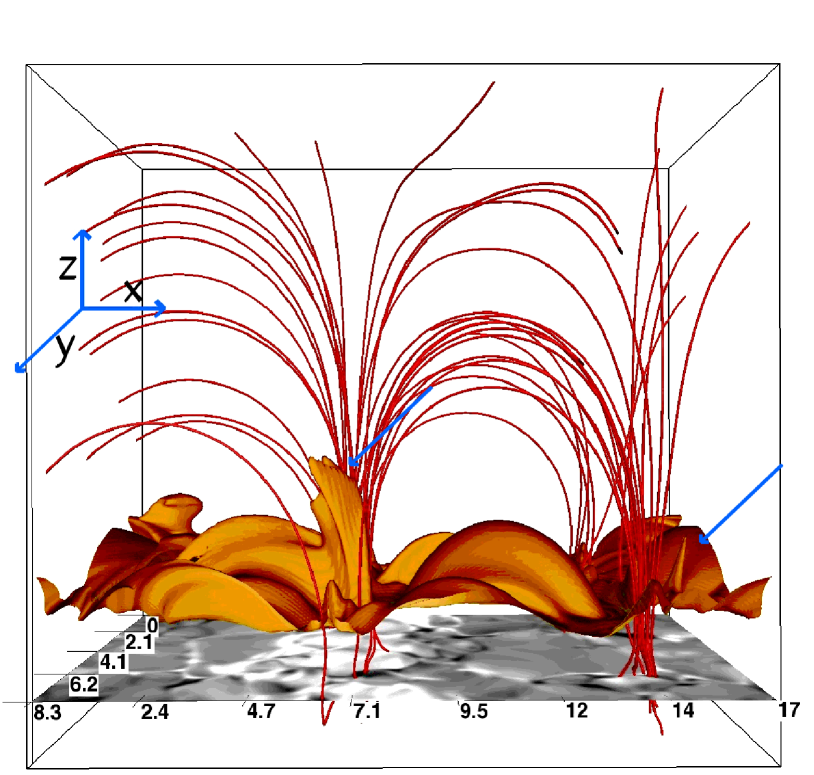
Figure 1: Magnetic field geometry and hydrodynamic configuration for the B1 simulation at $t=1850$ s: Field lines for the ambient pre-existing magnetic field (red), transition region surface at temperature $10^{5}$ K (orange isosurface), $B_{y}$ magnetic field component in the photosphere (grey scale with white $210$ G and black $-210$ G). Note the location of the simulated spicule of type ii in the transition region isosurface (blue arrow at $x\approx 7$ Mm) and the region of flux emergence in the photosphere (where $B_{y}$ is white). An example of a simulated type i is visible to the right (blue arrow at $x\approx 14$ Mm).

The model discussed in this paper is described in detail in Martínez-Sykora et al. (2009a, b), where it is labeled as model “B1”. The computational domain for this model stretches from the upper convection zone to the lower corona and is evaluated on a non-uniform grid of $256\times 128\times 160$ points spanning $16\times 8\times 16$ Mm³. The frame of reference for the model is chosen such that $x$ and $y$ are the horizontal directions, as shown in Fig. 1, which shows a selection of field lines, the $B_{y}$ component of the photospheric magnetic field, and the location of the transition region at time $t=1850$ s. The grid is non-uniform in the vertical direction ($z$-axis) to ensure that the vertical resolution is good enough to resolve the photosphere and the transition region with a grid spacing of 32.5 km, while becoming larger at coronal heights where gradients are smaller and scale heights larger. At this resolution the model has been run for roughly 1 hour solar time.

The initial model is seeded with magnetic field, which rapidly receives sufficient stress from photospheric motions to maintain coronal temperatures ($T>500\,000$ K) in the upper part of the computational domain, in the same manner as first accomplished by Gudiksen & Nordlund (2004). The initial field was obtained by semi-randomly spreading $20-30$ positive and negative patches of vertical field at the bottom boundary some $1.5$ Mm below the photosphere, then calculating and inserting the potential field arising from this distribution in the remainder of the domain. Stresses sufficient to maintain a minimal corona are built up by photospheric motions after roughly $20$ minutes solar time. The model has an average unsigned field in the photosphere of $160$ G and is distributed in the photosphere in two bands of vertical field centered around roughly $x=7$ Mm and $x=13$ Mm. In the corona this results in loop-shaped structures that stretch between these bands and are mainly oriented in the $x$-direction, as can be seen by following the red field lines shown in Fig. 1. Note that the time ($t=1850$ s) shown in the figure was chosen to coincide with the ejection of the spicule of type ii that is the subject of this paper. The jet is clearly visible in the isosurface that outlines the position of the transition region near $x=7$ Mm.

To start the events leading to the jets, we introduce a non-twisted magnetic flux tube into the computational domain through its lower boundary, that lies some $1.5$ Mm below the photosphere, as described in detail by Martínez-Sykora et al. (2008), section 3.2.

Horizontal magnetic flux of strength $10^{3}$ G is injected in a band of $1.5$ Mm of diameter parallel to the $y$-axis and centered at $x=8$ Mm at the bottom boundary. Hence, the injected magnetic field is nearly perpendicular to the orientation of the pre-existing ambient magnetic field outlined by the coronal loops that are seen in Fig. 1. The details of the input parameters of the simulation can be found in Martínez-Sykora et al. (2009b). The simulation has, therefore, on the one hand, a pre-existing field which interacts with granular convection similar to Abbett (2007); Isobe et al. (2008), and on the other hand, it has new emerging magnetic flux which is injected through the bottom boundary (Archontis et al., 2004; Cheung et al., 2007; Martínez-Sykora et al., 2008) and interacts with the granular convection and the pre-existing magnetic field.

4 Results

In the various simulations we have run, and in particular in the simulation discussed here, a large number of spicule-like structures are found. Most of these resemble spicules of type i, as described by Martínez-Sykora et al. (2009a). However, in addition, we also find jet-like structures that resemble spicules of type ii (Martínez-Sykora, 2010). These differ markedly in their physical characteristics from the pervasive type i.

Simulation B1 produced on the order of 100 spicules of type i. These spicules were found to result from upwardly propagating shocks passing through the upper chromosphere and into the transition region and corona. The shock-driven jets show up as narrow linear structures reaching some few Mm above the ambient chromosphere, rising and falling with velocities of order 30 km s^-1, and having lifetimes of order 3-5 minutes. An example of this type of jet is seen on the right-hand side of Fig. 1, (blue arrow near $x=14$ Mm) which appears like a narrow spike in the transition region. On the other hand, the simulation produced two jets that resemble spicules of type ii, but only two of them; one of these is shown in Fig. 1 as a prominent feature in the transition region (blue arrow near $x=7$ Mm). In this latter type of jet, chromospheric material is ejected far into the corona at very high velocity and heated, reaching velocities up to 95 km s^-1; the jet appears to fade without falling back towards the solar surface.

4.1 Structure

Both of the candidate spicules of type ii are located near the footpoints of coronal loops. Therefore, the field lines along which the jet is ejected are either open or, at least, penetrate far into the corona. Moreover, both jets appear near $x=7$ Mm (see blue arrow in Fig 1), close to locations where flux emergence is vigorous. In fact, we note that both jets first appear after the rising flux tube injected at the bottom boundary has emerged to and, in part, has crossed the photosphere.

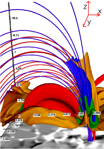
Figure 2: The structure of the type ii spicule and the related hot loop at $t=1850$ s, in terms of the temperature at $1.3\,10^{6}$ K (red isosurface), the transition region at $10^{5}$ K (orange isosurface), upflowing velocity along the field lines at $45$ km s^-1 (blue isosurface), and Joule heating at $1$ W/m³ (green isosurface). The field lines are drawn on opposite sides of the magnetic discontinuity in red and purple. $B_{y}$ at the photosphere is shown with a grey-scale map with a range of $[-210,210]$ G. Except in the spicule itself the transition region is on average some 2 Mm above the photosphere.

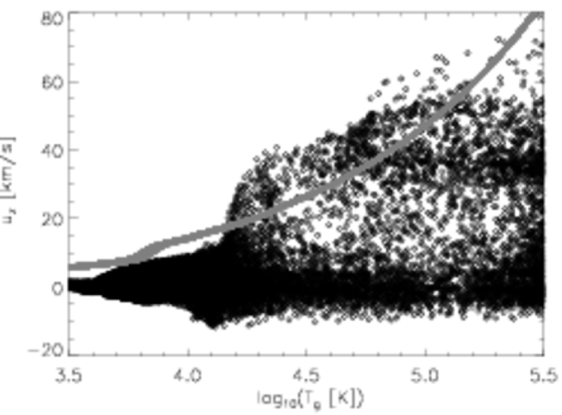
Figure 3: Distribution of vertical velocity $u_{z}$ as function of temperature $\log(T)$ in the vicinity of the spicule at time $t=1930$ s. Also shown with grey markers is the distribution of the speed of sound $c_{s}=\sqrt{{\gamma P/\rho}}$ at the same time. The spicule plasma is supersonic and has temperatures in the range from $15\,000$ K to some few $10^{5}$ K at this time in the evolution of the spicule.

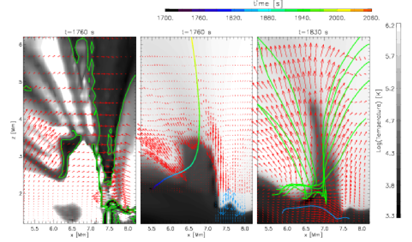
Figure 5: The spicule is formed as it is squeezed by the Lorentz force and material is ejected by the resulting pressure gradient. The ratio of Lorentz force to pressure gradient $|{\bf j}\times{\bf B}|/|\nabla P|]$ (grey scale left panel, black where the gas pressure gradient dominates), the green line shows where the ratio is equal to $1$. The temperature on a logarithmic scale at time $1760$ s, (grey scale middle and right panel) before the spicule ejection and at time $1830$ s (right panel). All panels are shown at the plane $y=6.02$ Mm. In the left panel the vectors show $({\bf j}\times{\bf B}/\rho)$ (red), in the middle panel $(\nabla P/\rho)_{||}$ (red and blue, the scale of the red vectors is half the value of the blue) and in the right panel the velocity field (red). Particle trajectories are shown in green (upflow) and blue (downflow) in the right panel. The particle trajectory shown as a function of time with the color-scheme in the middle panel is analyzed in detail in Fig. 6.

In Fig. 2, details of the type ii spicule structure are shown for the jet that is active at time $t=1850$ s in the B1 simulation: in the figure, isosurfaces for the upflow velocity (blue), temperature (orange: transition region; red: hot corona), and Joule heating per particle (green) are shown. The greyscale map towards the bottom of the figure corresponds to the horizontal magnetic field strength in the photosphere which clearly shows where flux emergence is vigorous. In addition, the figure shows magnetic field lines close to the jet structure. The jet is formed as chromospheric material is ejected into the corona and heated, with velocities reaching up to $95$ km s^-1. It is composed of many elements that together comprise a complicated phenomenon. In this paper, the spicule is identified with ejected material of chromospheric density and temperature, i.e. the jet-like structure seen in the orange temperature isosurface that appears next to the prominent spike seen in the blue velocity isosurface. The width of the jet is roughly $500$ km and its maximal length is around $4$ Mm, measured from the initial position of the transition region. The velocity of the ejected material in the jet is aligned (or very close to it) with the magnetic field and hence nearly vertical. The vertical component of the velocity along a vertical axis passing through the jet shows a vertically bipolar structure with center in the middle-chromosphere; i.e. above $z=1.5$ Mm upflow velocities are found while below this height material is downflowing (for details see section 4.3 and Fig. 5). The maximum downflow velocity is of order $10$ km s^-1. The upflowing ejected material has a distribution of velocities and temperatures: at its core it is cool, $15\,000$ K, and reaches velocities of $40$ km s^-1, but the blue velocity isosurface of Fig. 2 shows that there is warmer, faster upflow surrounding parts of the cool core with temperatures of a few $100\,000$ K, where the upflow velocity is higher than in the core, up to $95$ km s^-1. These numbers fits fairly well with the statistics of the RBE’s done by (Rouppe van der Voort et al., 2009). Further insight into the velocity structure can be found in Fig. 3 which shows the range of vertical velocities in the volume surrounding and including the jet as a function of temperature, along with the speed of sound ($c_{s}=\sqrt{{\gamma P/\rho}}$). The velocities comprising the jet are largely supersonic, with Mach numbers of order two for the lowest temperature gas.

Close to the base of the jet we find a region where the Joule heating per particle is large, as shown with the green isosurface in Fig. 2. Joule heating occurs along the entire length of the jet, but is strongest in the first few megameters near the base. As a result of Joule heating, the nearby corona is heated, and hot loops with temperatures up to 1.6 MK are produced with temperature much greater than that found in the ambient corona. These hot loops are apparent through the red temperature isosurface. Note that the hot loops have one footpoint near the base of the jet. The hot loops consist of low-density material, and are associated with, but separate from, the jet proper.

It is interesting to note that the magnetic field is unipolar in the region around the modeled jet; this is also the case for many observed spicules of type ii (McIntosh & De Pontieu, 2009). Even so, we find several regions with large gradients in the magnetic field in the chromosphere near the jet. More specifically, these discontinuities are found to be located inside a volume $2\times 2\times 3$ Mm³ at $[x,y,z]=[3:7,5:7,1.5:4.5]$ Mm. The region of magnetic discontinuities (i.e large magnetic field gradients or current sheets) is aligned with the $x$-axis. These gradients show a magnetic field topology that is similar to rotational discontinuities, with small inclinations between the field lines on either side of the gradient. These gradients produce the strong Joule heating at the footpoints shown with the green isosurface in Fig 2. The magnetic field configuration close to the jet is complex, and contains many locations with strong magnetic gradients. The jet is therefore not solely associated with a simple discontinuity, but rather with several locations of large electric currents.

It is important to note that the velocities in the upper part of the jet ($z>1.5$ Mm) are directed upward during the entire evolution. No downflows are found in the jet at any point in time, in contrast to the simulated spicules of type i, in which both up and downflows are found. The rapid fading of the jet at the end of its evolution is described in detail in section 4.4. A movie of the jet evolution is provided as on-line material accompanying this paper.

4.2 The photospheric precursor of the jet

A detailed description of the setup and evolution of the flux emergence in this simulation have been given in detail by Martínez-Sykora et al. (2008, 2009b). Martínez-Sykora et al. (2009b) demonstrated that flux emergence causes the magnetic field to expand into the corona, and that this expansion produces discontinuities in the coronal field. We believe that this also applies to the regions of large magnetic field gradient obtained in the present paper. These discontinuities are the source of the Joule heating which produces the hot loops, and have the indirect consequence of producing the jet upflow, as described below.

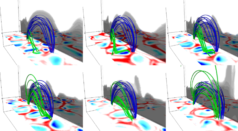
Figure 4: Horizontal magnetic field emerges through the photosphere in granules and accumulates in the intergranular lanes. The red-blue surface at the photosphere shows the vertical velocity (red is downflow and blue is upflow with range [-2,2] km s^-1). The grey-scale surface shows the temperature in logarithmic scale in the $xz$-plane at $y=6$ Mm. The green magnetic field lines follows the bulk of plasma that emerges from the photosphere and expands into the corona. The blue field lines are taken at the same region in all timesteps near the upper chromosphere. The time series is t=[850,1050,1200,1300,1550,1900] s from left to right and top to bottom.

We have located emergence events in individual granules at the photosphere that are likely precursors of the jet described in the other sections. The sequence of images shown in Fig. 4 shows one such event. In the six panels comprising the figure we illustrate the emergence and gradual blending of a set of field lines (green lines) with a set of field lines representing the pre-existing field in the vicinity of the jet (blue lines). Also shown is the velocity field in the photosphere, i.e. at height $z=0$ Mm, and the logarithm of the temperature in an $x-z$ plane placed at $y=6$ Mm (this is the same plane used to describe the jet in Fig. 5). In the upper left panel, at $t=850$ s, the emerging field within a granule (see the horizontal component in the photosphere of the green lines) shows one footpoint connected to the convection zone, while the other footpoint is linked somewhere below the photosphere to field lines that expand into the chromosphere, forming loops that are oriented at an angle to the pre-existing field. In the top center panel, at $t=1050$ s, these field lines are seen to connect to newly emerged horizontal field oriented in the $y$-direction with footpoints near the pre-existing field foot points. As the emerging field continues to rise into the chromosphere, shown in the top right and bottom left panels at $t=1200$ s and $t=1300$ s respectively, the strong hairpin curve in the emerging field is seen to become shallower as the field straightens and the field lines begin to blend with the pre-existing field lines. In the bottom center panel, at $t=1550$ s, the hairpin has largely disappeared and at the same time we see the first evidence of the jet in the temperature plot to the right and above the displayed field lines. The bottom right panel, at $t=1900$ s, shows the emerging field lines expanding and interacting with the pre-existing field and that cool gas has been ejected into the corona to the right of the system of field lines shown.

The evolution of the field lines shows they presumably have suffered reconnection before appearing at the surface: while in the granule interior, emerging field lines seem to have reconnected with the pre-existing field resulting in the hairpin configuration of the emerging field lines. Hybrid field lines (drawn in green in Fig. 4) result, linking the emerging system in the granule interior with the pre-existing ambient coronal field, and with the high-curvature stretch near the location where the reconnection is likely to have occurred. The high-curvature portion of these field lines has a sharp hairpin shape which is difficult to reconcile with having resulted from processes other than reconnection, such as e.g., the deformation caused by the granular flows. This early reconnection may take place at different heights in the granule interior but in any case in high plasma-$\beta$ ($1$ Mm below the photosphere) and it therefore does not have the spectacular consequences often associated with low plasma-$\beta$ reconnection; ie. no jets or flows. This kind of process might occur not only in the quiet sun, network or internetwork, but also in plage, where the field is mostly unipolar. Since our primary interest is to understand the consequences of these severely deformed field lines as they emerge into the chromosphere, we will not study the sub-surface reconnection in detail, only mention that this (or similar processes) can produce complex magnetic field configurations in the high plasma-$\beta$ part of the atmosphere that can survive emergence into the chromosphere.

Photospheric footpoint motions and high curvature lead to large magnetic field gradients and eventually a reorientation of the field in the chromospheric and coronal layers which is the ultimate source of the jet described in detail in section 4.3. As mentioned above, the emerged field lines and the pre-existing field form an angle to each other and a geometry similar to a rotational discontinuity, but the change in the orientation is small. Though we see Joule heating, such a small inclination may not be large enough to produce dynamically significant reconnection in the chromosphere.

In the simulation, only a few granules show field configurations of sufficient complexity to lead to discontinuities in the overlying chromosphere. Hence, only a few jets of the type discussed here are formed and launched during the entire numerical experiment.

4.3 Source and connectivity

The large magnetic field gradients in the chromosphere described in section 4.1 do not produce an upflow jet, but rather horizontal flow, and the acceleration associated with the discontinuity is small. How then can jets that pull chromospheric material up to $7$ Mm above the photosphere at velocities $>60$ km s^-1 be produced? In Fig. 5 and 6 we show various aspects of the force balance in the vicinity of the jet that occurs near $t=1850$ s. The arrows in Fig. 5 correspond to the Lorentz acceleration (left panel), the pressure gradient acceleration along the field lines before the jet is launched (middle panel) and the velocity field when the jet is launched (right panel). The grey scale map in the left panel compares the absolute value of the Lorentz force and the pressure gradient, just before the jet is formed at $t=1760$ s (white means that the Lorentz force is larger than the gradient of pressure). The temperature is shown with the grey-scale map in the middle panel at $t=1760$ s and in the right panel at $t=1830$ s, when the jet has evolved. These plots imply that the chromospheric material actually is thrown into the corona by a gas pressure gradient, after being initially accelerated horizontally by the Lorentz force.

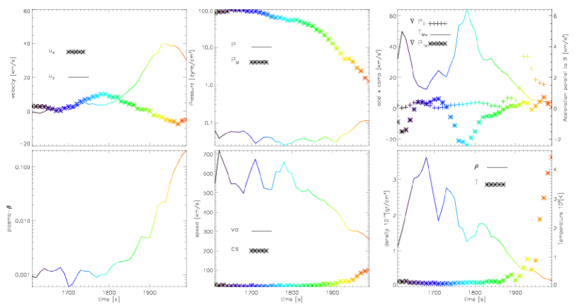
Figure 6: Different quantities evolution as a function of time of the particle which path is shown in the middle panel of Fig. 5. The vertical (solid line) and $x$-component (asterisk symbols) of the velocity are shown in the top-left panel. Plasma-$\beta$ is shown in the bottom-left panel. The gas pressure (solid line) and magnetic pressure (asterisk symbols) are shown in the top-middle panel. Alfvén (solid line) and sound speed (asterisk symbols) are shown in the bottom panel. The acceleration in the $x$-direction due to the magnetic tension ($(B\nabla)B/(2\rho\mu)$, solid line, left vertical axis), due to the gradient of the magnetic pressure (asterisk symbols, left vertical axis), and due to the pressure gradient along the field of lines (plus symbols, right vertical axis) are shown in the top-right panel. Density (solid line) and temperature (asterisk symbols) are shown in the bottom-right panel. The color scheme corresponds to the time and is the same as in Fig. 5.

That the cold material found at great heights is indeed the result of an ejection from the chromosphere can be seen by studying the particle trajectories of material composing the jet, shown as green, blue, and multicolored lines in the middle and right panels of Fig. 5. Particles clearly start in the chromosphere before being ejected to coronal heights. The velocity field after the jet is formed, at $t=1830$ s, is shown in the right panel of Fig. 5. The velocity has a positive horizontal gradient in the chromosphere on the left side of the cold jet that has formed. The horizontal $x$-component of the velocity also increases with time at chromospheric heights in locations near the jet. Figure 6 shows the vertical and $x$-component of the velocity for the trajectory shown in the middle panel of Fig. 5. The particle horizontal velocity increases with time, in the interval from 1700 (purple) to 1800 s (blueish). Then, the particle is deflected and $u_{z}$ increases considerably, up to 40 km s^-1. The particle evolves under chromospheric conditions during this time material and the temperature remains below $10^{5}$ K (see right-bottom panel) until $t=1930$ s. Note that Fig. 3 shows that there are many particles ejected with velocities of the order of 40 km s^-1 and temperature of the order $10^{4}$ K, as well as particles with 60 km s^-1 and temperature of the order of $10^{5}$ K. Observe that plasma-$\beta$ (left-bottom panel) is below $10^{-2}$ when the particle is accelerated along the $x$-direction, after which plasma-$\beta$ increases to $0.1$. We can also see the large difference between the magnetic pressure and the gas pressure in the middle-top panel. Therefore, the Alfvén speed is of the order of 500 km s^-1 and the sound speed around 20 km s^-1 (see middle-bottom panel), i.e. the plasma is highly magnetized and the horizontal force balance roughly perpendicular to the field is completely dominated by the Lorentz force.

In order to find out what drives to the plasma to be squeezed in and later ejected from the chromosphere, examine the left panel of Fig 5: there are two regions where the Lorentz acceleration is larger than the pressure gradient, one inside the cold jet material and the other one $0.5$ Mm further to the right ($x>7.7$ Mm). The plasma is squeezed between these two regions. The Lorentz force located to the left side and inside the jet ($x<7.5$ Mm) is produced by the strong magnetic field gradients, where the field lines show a small jump in the magnetic field line orientation. This type of gradient produces a current that flows in the $y$-direction. The magnetic field is mainly vertical, oriented along $z$, and thus a strong Lorentz force results that points horizontally in the $x$-direction as shown by the red vectors inside the white area delineating the jet in the left panel of Fig. 5. Making a decomposition between the magnetic tension and the gradient of magnetic pressure along the $x$-direction, we can see in the top-right panel of Fig. 6 that the particle suffers a strong magnetic tension in the $x$-direction. This panel shows the time evolution the magnetic tension and the total (gas and magnetic) pressure gradient in the horizontal direction for a specific particle (see the trajectory in the middle panel of Fig. 5), This magnetic tension, which comes from the expansion of the emerging field lines, is the force which pulls the plasma to the right and squeezes it.

Thus, the magnetic tension component of the Lorentz force is the active agent that moves the plasma from left to right in the $x$-direction. The Lorentz acceleration is by far the most important component in the region where the particles move horizontally, to the left of, and inside the jet. Clearly, the magnetic tension is the force that squeezes the plasma and increases the pressure. We want to clarify that the agent of the magnetic tension in the chromosphere is due to the expansion of the emerging field lines. We could not find any clear reconnection, nor tangential discontinuities, i.e. the largest inclination between the emergent magnetic field and the ambient magnetic field lines are smaller than 10 degrees. Therefore, any subsequent reconnection with such variation in the angles between the field lines can hardly be the source of the strong magnetic tension.

Considering only the Lorentz acceleration, and integrating along the particle path for a particle moving along its trajectory until it reaches the region where it is ejected upward gives a velocity that is supersonic. The resulting particle trajectory is horizontal and the particles moves a distance on the order of $2$ Mm, as shown with the green lines in the right panel of Fig. 5. In the actual modeled case we find that the cool jet plasma is moving horizontally with nearly the speed of sound before it is deflected in the vertical direction as shown in the upper left panel of Fig. 6.

It is interesting to note that the Lorentz force squeezes the cold chromospheric plasma into a rather narrow structure. The flow above a specific vertical height is upward while the velocity is directed downward below this height (see right panel of Fig. 5). However, what force deflects the flow in a vertical direction and pushes the plasma into the corona? The top right panel of Fig. 6 also shows the gas pressure gradient parallel (almost vertical) to the magnetic field, where there is no Lorentz force. Initially, the particle is accelerated horizontally by the Lorentz force and the horizontal velocity becomes nearly supersonic. However, when the particle gets closer to the region where the plasma is being squeezed, both the gas pressure gradient and the magnetic pressure gradient act against this flow. The gas pressure gradient becomes large along the field lines, with no resistance to motion other than the gravity. In some places the pressure gradient acceleration reaches values nearly 10 times larger. For the particular particle track shown in Fig 6 we find that the vertical velocity increases by 20 km s^-1 between $t=1850$ s and $t=1910$ s, while in the same period the temperature is remains below $30\,000$ K. Integrating ${(\nabla P)_{\parallel}/\rho}-g$ over the same period gives 16 km s^-1: most or all of the vertical velocity increase is due the pressure gradient along the field and we conclude that while the horizontal force balance is dominated by the Lorentz force; the gas pressure gradient plays an important role in turning the horizontal gas flow and especially in accelerating the jet vertically. The jet has a complex 3D structure, and the different forces, velocities, heating and accelerations are not located in the same position, it is therefore quite difficult to follow in only one particle all the processes which happen in the spicules, but we note that already at time 1820 s the gradient of pressure is more than five times larger than gravity.

On the right side of the jet, at the boundary between the cool chromospheric material of the jet and coronal temperatures, the horizontal flow reaches a “wall” where the pressure gradient takes over, and the material is accelerated vertically (see dark region in the right side of the jet in the left panel of Fig. 5). This pressure gradient is large enough to push the flow up to heights 7 Mm above the photosphere. The wall on the right side of the jet that forces an increase in the pressure is due to the Lorentz force (see vectors at the right side of the jet in the left panel of Fig. 5). This wall is not of the same nature as the Lorentz force on the left and inner side of the jet, as there is no horizontal flow nor large magnetic field gradients associated with it, but the hot plasma there is magnetically dominated ($\beta<<1$) and the vertical magnetic field has a much larger energy density than that contained in the plasma that is colliding with the magnetic field forming the wall. The wall concentrates the plasma on the right side of the jet and thus increases the pressure, producing a deflection of the flow. The jet slowly moves to the right with time (see middle and right panel of the Fig. 5), along with the wall itself and the region where the plasma is squeezed and forced to move vertically.

That the horizontal flow of the jet is deflected by the pressure gradient is also illustrated with the vectors drawn in the middle panel of Fig. 5. These vectors are over-plotted on an image of the temperature structure in the vicinity of the jet just before the ejection. The vectors show that there are mainly two regions where the flow is strongly deflected by the pressure gradient; centered near $[x,z]=[6.0,2.9]$ Mm and near $[x,z]=[7.3,1.5]$ Mm, both aligned with the magnetic field. The leftmost of these regions is located above the transition region where, later in time, a hot loop will appear. The other region lies to the right, and it is from this latter region the cool jet rises. Observe that the region of large pressure gradient is not concentrated in one small spot but stretches a long distance along the jet and the hot loop. The plasma flow in the earlier stages (left and middle panels of Fig. 5) of the event is more concentrated towards the right-hand side of the boundary between the chromospheric and coronal material than it is in later stages (right panel) which shows strong upflows in regions closer to the left side of the jet. It is important to understand that even though the plasma-$\beta$ is low, the pressure gradient is aligned with the magnetic field lines and thus dominates the dynamic along the field. Therefore, as mention above, the pressure gradient is free to accelerate the plasma into the corona. We find that the magnetic tension squeezing of the plasma increases the pressure in some regions by as much a factor 10, as seen in the middle upper panel of Fig 6. Subsequently, note that the cool jet plasma is far from following the elementary adiabatic law $P\propto T^{\gamma/(\gamma-1)}$: helium is ionized at some $10\,000$ K, increasing the number of particles, on the other hand the ionization process costs energy and the temperature remains fairly constant until ionization is complete. Only when the gas is fully ionized does the temperature increase as rapidly as predicted in the elementary adiabatic case. While the gas pressure increase is of the order of 10 times in the chromosphere the temperature increase is no more than a factor 1.4 during the most vigorous part of the compression. The combination of large horizontal inflow velocities, ionization/recombination processes and magnetic squeezing results in a greater vertical velocity than would otherwise be predicted (Shibata et al., 1982; Shibata & Suematsu, 1982).

The tension force that drives the horizontal motions is a consequence of the magnetic field that penetrates into the chromosphere. This field is a result of the reconfiguration in the photosphere due to previous reconnection and emergence. As described earlier strongly bent field lines expand into the chromosphere and butt against the previously existing field. Note that, in the chromosphere the difference in orientation between the emerging field and the pre-existing field is small (less than 30 degrees). The emerging field lines are not in equilibrium and penetrate high into the upper chromosphere (see Fig. 4). The magnetic tension that squeezes the plasma and drives the jet results from this expansion of field lines that are not well aligned with the previously existing ambient field. The current sheets that form between these flux systems are also the sites of enhanced Joule heating and potentially of reconnection. However, we have not found any clear evidence of reconnection at the chromospheric level, and since the relative angle between the magnetic field systems is small, it seems unlikely that eventual hidden reconnection dominates the jet dynamics.

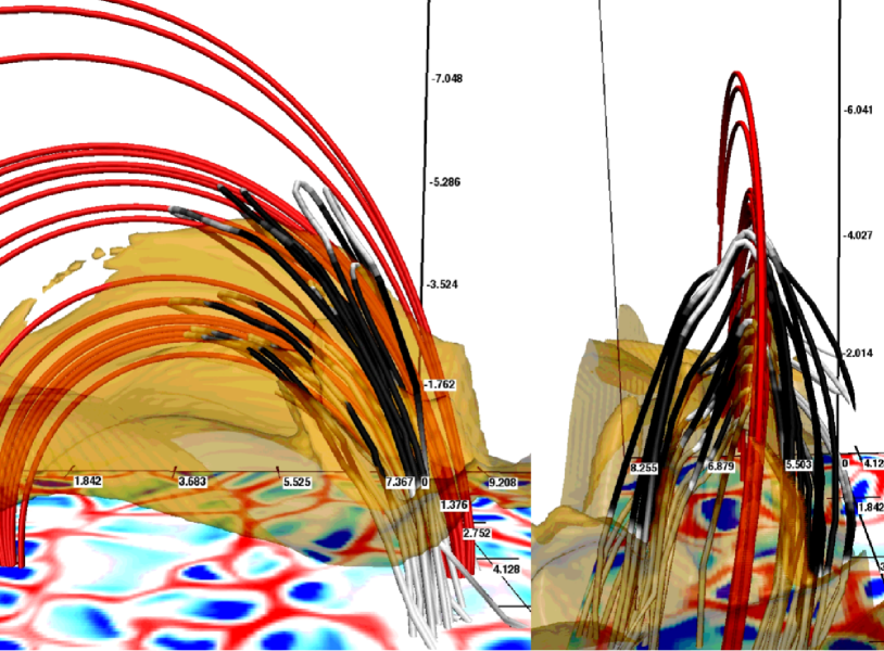
Figure 7: The structure and properties of the modeled spicule and its vicinity are connected with the configuration of the electric current and magnetic field. The field lines of the electric current are drawn with black-white colors, where black and white indicate low and high Joule heating respectively. The magnetic field are drawn with red lines. The transition region ($10\,^{5}$ K) is indicated using an orange semitransparent isosurface. The photospheric vertical velocity is shown in a blue-red colored map with range $[-2,2]$ km s^-1.

How do all these different structures; the upflows, the hot loop and the ejected chromospheric material, connect from the photosphere up to the corona? Is there any clear link between them? and why are they formed next to each other? The link between them lies with the orientation of the electric current as compared to that of the magnetic field lines, as shown in Fig. 7. The magnetic field configuration in combination with the current field distributed spatially in the surroundings of the jet is complex and difficult to visualize. In the vicinity of the footpoints of the ejected chromospheric material we find a region of large Joule heating per particle (white colored region of the current lines near $(x,y,z)=(7,5:8,1.7)$ Mm). The current lines in this region are mainly parallel to the magnetic field lines, this is where the gradient shows a topology of the field lines similar to a rotational discontinuity with a small relative angle. Following the current field lines higher up in the structure the heating per particle is reduced (black region of the current lines, around $(x,y,z)=(6,5:8,2.3)$ Mm), where the current lines are still parallel to the field lines. Following the current field lines even further, the Lorentz force becomes important where ${\bf J}$ forms a large angle to ${\bf B}$, which is seen to occur near the apex of the rendered current lines, where the current changes direction and becomes perpendicular relative to the magnetic field. Here the ${\bf J}$ is nearly perpendicular the current is large again (white small region at the top of the current field lines, around $(x,y,z)=(5,6.9,3.5)$ Mm). Therefore, regions of large Lorentz force and regions of large Joule heating per particle lie next to each other, but do not overlap.

4.4 Fading away

Roughly one minute after the jet is ejected into the corona the cold material contained in it starts to disappear. This material does not fall down again, instead it expands into the corona where it is heated to coronal temperatures. This process takes only a few tens of seconds.

The heating associated with the jet is concentrated mostly in a region close to the footpoint of the cold jet. The different heating and cooling contributions are shown in Fig. 8 as a function of time. We calculated the mean value in a volume of roughly $1$ Mm³ for each heating contribution. The volume is centered at the footpoint of the jet. The only component that contributes to the heating is the $Q_{J}$, since the compression heating ($P\nabla{\bf u}$) contributes mainly under expansion, i.e. it is cooling. Therefore, the important heating mechanism that heats the chromospheric material up to coronal temperature is the Joule heating. The Joule heating in this volume is large enough to heat all the mass that is injected into the corona ($4.9\,10^{7}$ kg, see section 4.5) up to temperatures of the order $10^{6}$ K. Assuming that we heat the gas in a cubic volume that spans $x=[6.3,7.2],y=[5.8,6.7]$ and $z=[3.54,2.54]$ Mm from chromospheric to coronal temperatures ($T\approx 10^{6}$ K and $\rho\approx 2\,10^{-14}$ gr cm^-3) we estimate that this requires $(3/2)k_{b}(\rho/m)T\approx 2.5\,10^{24}$ ergs. Comparing this to an average Joule heating in the same volume measured to be $2.6\,10^{22}$ erg s^-1, we find that Joule heating contributes $2.6\,10^{24}$ ergs during the 100 s of the jet lifetime. The heating comes from the patches of Joule heating (see Fig. 2) that both produce the hot loop and heat the adjacent chromospheric material as it ascends. This injected energy also propagates along the field lines through conduction, once the plasma has reached sufficient temperature to make thermal conduction efficient, raising the temperature even in upflowing material far from the heating site.

In the earlier stages of the ejection the density is high and the Joule heating per particle is low. However, as the density of the cool chromospheric material decreases during expansion, the heating rate per particle increases rapidly and the temperature of the material rises. The volume where Joule heating is large grows with the jet and is present until the discontinuities in the magnetic field are relaxed and the current becomes insignificant.

As mentioned previously the acceleration along the magnetic field lines is due to the gas pressure gradient. This increase in pressure is due to squeezing of the chromospheric plasma rather than by Joule heating. We have checked that the entropy increase in the plasma being accelerated is comparatively small: the largest entropy increase is located to the sides of the ejected chromospheric material. It is there, rather than in the jet itself, that the Joule heating per particle is largest.

4.5 Mass and enthalpy flux associated with the jet

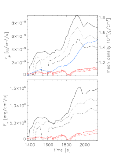
Figure 9: Chromospheric material is injected into the corona. Mass flux (top panel) and energy flux (bottom panel) for the chromospheric material of the jet structure (black lines) and in the corona (red lines) as a function of time, shown at $z=[3.4,4.1,5]$ Mm above the photosphere (solid, dotted, and dash-dotted lines respectively). The mean density in the corona ($T>10^{5}$ K) is shown in blue in the top panel.

Spicules inject mass, momentum, and energy into the corona. The mass flux at fixed heights ($z=[3.4,4.1,5]$ Mm) is shown in the top panel of Fig. 9. Red lines correspond to the total flux in regions with coronal temperatures (more precisely: $T>10^{5}$ K) and black lines correspond to the chromospheric material of the jet (i.e., points with $T<10^{5}$ K and restricted to the vicinity of the jet). The flux per unit of area is calculated as follows:

$$F_{\rho}=\frac{\int_{S}(\rho\,u_{z})ds}{\int_{S}ds}\;,$$ (1)

$$F_{e}=\frac{\int_{S}(u_{z}\,e)ds}{\int_{S}ds}\;,$$ (2)

where $\rho$ is the density, $u_{z}$ is the vertical velocity, and $e$ is the internal energy per unit volume. During the $700$ s displayed, the mass flux is always positive. Most of it is due to the injection and heating of chromospheric material from the jet(s). We see two phases in the figure, coinciding with two jet ejections: one starting at around $t=1400$ s, and the other, which has been the focus of this paper, starting at time $1750$ s. The mass flux per unit area in the jet (black lines) reaches a value more than 4 times greater than the average inflow through high temperature points (red lines). The mass injected into the corona by the jet along its $100$ s lifetime is on the order of $4.9\,10^{7}$ kg.

In addition to mass, a large amount of thermal energy is also injected into the corona. The enthalpy flux is shown in the bottom-panel of Fig. 9 which follows the same color and line-type scheme as the top panel. The largest thermal energy inflow by the jet starts at time $1750$ s and is at least $3$ times greater than that entering the rest of the corona; the total thermal energy injection by the jet is about $8\,10^{24}$ erg during its lifetime (De Pontieu et al., 2011).

The mean density in the corona is shown in blue in the top-panel of Fig. 9. The mean density is calculated to be the total coronal mass divided by the coronal volume, defined as the volume in which the temperature is greater than $10^{5}$ K. The mean density in the corona increases considerably as the jet supplies mass into the high temperature regions of the upper atmosphere.

5 Discussion and conclusions

We have studied the physics and dynamics of a plausible candidate for a type ii spicule model found in realistic 3D simulations. This candidate evolved naturally as a consequence of the dynamics of the model. The mechanism is complex: chromospheric material is ejected into the corona as plasma is pushed horizontally by a strong Lorentz force towards a “wall” of strong vertical magnetic field where plasma-$\beta<1$. The wall causes a large increase in the pressure and thus deflects the plasma and forces it to flow vertically along the magnetic field, most rapidly towards the low densities of the corona. The compression does not follow the elementary adiabatic process, because, mostly, helium is ionized and the temperature remains fairly constant during the process. The Lorentz force which pushes the plasma results from large gradients in the field orientation that have accumulated in the upper chromosphere. These large gradients possess a current that is both horizontal and perpendicular to the magnetic field depending the spatial position and time.

This mechanism cannot be identified with previous mechanisms described in the literature; it is different from the surges caused by propagating shocks (Shibata & Suematsu, 1982; Shibata et al., 1982) or the spicules described by Hansteen et al. (2006); Heggland et al. (2007); Martínez-Sykora et al. (2009a) among others. Such phenomena come from a shock which is formed in or crosses the chromosphere and pushes the transition region upwards. The mechanism discussed here is also different from the cases of collision of emerging plasma with a preexisting ambient magnetic field in the corona that lead to a large magnetic field discontinuity (Yokoyama & Shibata, 1996; Archontis et al., 2005; Galsgaard et al., 2007; Moreno-Insertis et al., 2008; Nishizuka et al., 2008, among others). Such simulations show that reconnection can produce a strong jet when the outflows from the reconnection site impinge upon the neighboring medium with subsequent squeezing of the plasma and acceleration along the field lines. At first sight the phenomena described in this paper could seem to have common features with that mechanism. However, in our simulation the reconnection, the collision and the plasma squeezing take place in quite different layers, from the convection zone to the chromosphere. The primary cause of the modeled type ii spicule in our model is not reconnection in the chromosphere, but rather the squeezing caused by the straightening and expansion of field lines rising from the photosphere.

The ultimate source of the strong magnetic field gradients in the upper chromosphere is the local emergence of magnetic flux that injects strongly stressed magnetic fields into the photosphere just below the site of the ejected jet. The main effect is the interaction between the flux emerging in the granules and the intergranular ambient field: the former suffer a reorientation while the lines connected to the intergranules do not. As they rise into the upper layers of the atmosphere the former field lines show strong magnetic tension. These two system of field lines are the source of large gradients of the magnetic field orientation that arise higher in the upper chromosphere with large current along the field of lines and Joule heating.

Joule heating near the footpoints of the ejected spicule initially produces a hot loop to the side of the ejection, where the heat is spread throughout the loop by thermal conduction. Later in time, this same heating also raises the temperature of the cool spicule material to coronal values, in fact on a fairly short time scale (on the order of a few tens of seconds) once the chromospheric material has expanded into the corona.

Such processes have considerable effects on the modeled corona which potentially could be important. For instance, we observed a large injection of chromospheric material into the corona and an accompanying thermal energy flux sufficient to significantly contribute to heat the corona. In addition, large upflow velocities are introduced into the lower corona that carry a substantial kinetic energy flux.

It is worth mentioning that the large magnetic field gradients needed to create the conditions necessary to accelerate the spicules discussed in this paper could alternately be produced by other sources than flux emergence; for example one could imagine that chromospheric dynamics in the high plasma-$\beta$ region of the atmosphere potentially could stress the magnetic field sufficiently. However, in the model analyzed here we could only find candidate type ii spicules that were related with flux emergence. This might be because the initial field configuration is severely simplified in the model compared to topologies found in the actual sun and/or that the chromospheric model presented here could be improved, through better spatial resolution or by adding other relevant physics beyond MHD. Thus, one important avenue of research is to analyze which magnetic field topologies are most likely to produce spicules of type ii: the quiet sun, plage, or active regions. Alternatively, one could determine what other sources could lead to the development of large magnetic field gradients in the chromosphere. Another avenue is to consider how the resolution in the chromosphere and corona limits the width of possible spicule and the violence of dynamics at small scales. Other physical process that might affect the dynamics is the inclusion of a generalized Ohm’s law. A necessary prerequisite in this case is to treat the ionization of hydrogen in a time dependent manner, which in and of itself will also have profound effects on chromospheric dynamics as discussed in detail by (Carlsson, 2009; Leenaarts, 2010; Martínez-Sykora, 2010).

Nevertheless, we have demonstrated here that the combination of strong Lorentz forces in particular magnetic field geometries in the upper chromosphere can produce high velocity jets of cool material along the magnetic field into the corona that share several characteristics with observed spicules of type ii.

6 Acknowledgments

This research has been supported by a Marie Curie Early Stage Research Training Fellowship of the European Community’s Sixth Framework Programme under contract number MEST-CT-2005-020395: The USO-SP International School for Solar Physics. Financial support by the European Commission through the SOLAIRE Network (MTRN-CT-2006-035484) and by the Spanish Ministry of Research and Innovation through projects AYA2007-66502 and CSD2007-0050 are gratefully acknowledged. Supported through grants SMD-07-0434, SMD-08-0743, SMD- 09-1128, SMD-09-1336, and SMD-10-1622 from the High End Computing (HEC) division of NASA.

The 3D simulations have been run with the Njord and Stallo cluster from the Notur project. We thankfully acknowledge the computer and supercomputer resources by Research Council of Norway through grant 170935/V30 and through grants of computing time from the Programme for Supercomputing. This work was made possible by NASA s High-End Computing Program. In addition, the simulation presented in this paper was carried out on the Columbia cluster at the Ames Research Center. We thank the Advanced Supercomputing Division staff for their technical support.

To analyze the data we have used IDL and Vapor (http://www.vapor.ucar.edu).

We would like to thank to the referee, whose comments helped us to improve the manuscript considerably. We also thank Bart de Pontieu for the nice discussions on the topic of this paper.

Figure 8: Energy balance is shown as a function of time at the footpoint of the spicule. Mean value around the footpoint (centered at $(x,y,z)=(6.8,6.2,3)$ Mm and the mean is calculated within a volume of $1$ Mm³) of the spicule of the advection of energy ($\nabla e{\bf u}$, dashed line), radiative loss ($Q_{r}$, dot-dot-dot-dashed line), Joule heating ($Q_{J}$, dot-dashed line) and compression heating ($P\nabla\bf{u}$, solid line, note that this term is negative, energy lost) are shown as a function of time. The plasma at the footpoint of the spicule is heated by Joule heating.

References

- Abbett (2007) Abbett W. P., 2007, ApJ, 665, 1469
- Archontis et al. (2004) Archontis A., Moreno-Insertis F., Galsgaard K., Hood A., O’Shea E., 2004, A&A, 426, 1047
- Archontis et al. (2005) Archontis V., Moreno-Insertis F., Galsgaard K., Hood A. W., 2005, ApJ, 635, 1299
- Beckers (1968) Beckers J. M., 1968, Sol. Phys., 3, 367, Solar Spicules (Invited Review Paper)
- Carlsson (2009) Carlsson M., 2009, Memorie della Societa Astronomica Italiana, 80, 606
- Carlsson & Stein (1992) Carlsson M., Stein R. F., 1992, ApJ, 397, L59
- Carlsson & Stein (1994) Carlsson M., Stein R. F., 1994, en Carlsson M. (ed.), Chromospheric Dynamics, p. 47
- Carlsson & Stein (1997) Carlsson M., Stein R. F., 1997, ApJ, 481, 500
- Carlsson & Stein (2002) Carlsson M., Stein R. F., 2002, ApJ, 572, 626
- Cheung et al. (2007) Cheung M. C. M., Schüssler M., Moreno-Insertis F., 2007, A&A, 467, 703,
- De Pontieu et al. (2007a) De Pontieu B., Hansteen V. H., Rouppe van der Voort L., van Noort M., Carlsson M., 2007a, ApJ, 655, 624
- De Pontieu et al. (2007b) De Pontieu B., McIntosh S., Hansteen V. H., et al., 2007b, PASJ, 59, 655
- De Pontieu et al. (2011) De Pontieu B., McIntosh S. W., Carlsson M., et al., 2011, Science, 331, 55
- De Pontieu et al. (2007c) De Pontieu B., McIntosh S. W., Hansteen V., Carlsson M. P., 2007c, AGU Fall Meeting Abstracts, C8, Hinode and the Corona’s Lower Boundary: Spicules and Alfvén Waves
- De Pontieu et al. (2009) De Pontieu B., McIntosh S. W., Hansteen V. H., Schrijver C. J., 2009, ApJ, 701, L1
- Dorch & Nordlund (1998) Dorch S. B. F., Nordlund A., 1998, A&A, 338, 329
- Emonet & Moreno-Insertis (1998) Emonet T., Moreno-Insertis F., 1998, ApJ, 492, 804,
- Galsgaard et al. (2007) Galsgaard K., Archontis V., Moreno-Insertis F., Hood A. W., 2007, ApJ, 666, 516
- Gudiksen & Nordlund (2004) Gudiksen B. V., Nordlund Å., 2004, An Ab Initio Approach to the Solar Coronal Heating Problem, en IAU Symposium, Vol. 219, Dupree A. K., Benz A. O. (eds.), Stars as Suns : Activity, Evolution and Planets, p. 488
- Hansteen et al. (2006) Hansteen V. H., De Pontieu B., Rouppe van der Voort L., van Noort M., Carlsson M., 2006, Apj, 647, L73
- Heggland et al. (2007) Heggland L., De Pontieu B., Hansteen V. H., 2007, ApJ, 666, 1277
- Heggland et al. (2009) Heggland L., De Pontieu B., Hansteen V. H., 2009, ApJ, 702, 1
- Hyman et al. (1979) Hyman J., Vichnevtsky R., Stepleman R., 1979, Adv. in Comp. Meth, PDE’s-III, 313
- Isobe et al. (2008) Isobe H., Proctor M. R. E., Weiss N. O., 2008, ApJ, 679, L57
- Judge & Meisner (1994) Judge P. G., Meisner R. W., 1994, The ‘HAO spectral diagnostics package’ (HAOS-Diaper), en ESA Special Publication, Vol. 373, Hunt J. J. (ed.), Solar Dynamic Phenomena and Solar Wind Consequences, the Third SOHO Workshop, p. 67
- Kosugi et al. (2007) Kosugi T., Matsuzaki K., Sakao T., et al., 2007, Sol. Phys., 243, 3, The Hinode (Solar-B) Mission: An Overview
- Langangen et al. (2008) Langangen O., De Pontieu B., Carlsson M., et al., 2008, ApJ, 679, L167
- Leenaarts (2010) Leenaarts J., 2010,Mem. Soc. Astron. Italiana, 81, 576
- Mackay & Galsgaard (2001) Mackay D. H., Galsgaard K., 2001, Sol. Phys., 198, 289
- Martínez-Sykora (2010) Martínez-Sykora J., 2010, ArXiv e-prints, 2 types of spicules ”observed” in 3D realistic models
- Martínez-Sykora et al. (2008) Martínez-Sykora J., Hansteen V., Carlsson M., 2008, ApJ, 679, 871
- Martínez-Sykora et al. (2009b) Martínez-Sykora J., Hansteen V., Carlsson M., 2009, ApJ, 702, 129
- Martínez-Sykora et al. (2009a) Martínez-Sykora J., Hansteen V., DePontieu B., Carlsson M., 2009, ApJ, 701, 1569
- Matsumoto & Shibata (2010) Matsumoto T., Shibata K., 2010, ApJ, 710, 1857
- McIntosh & De Pontieu (2009) McIntosh S. W., De Pontieu B., 2009, ApJ, 706, L80
- Moreno-Insertis et al. (2008) Moreno-Insertis F., Galsgaard K., Ugarte-Urra I., 2008, ApJ, 673, L211
- Nishizuka et al. (2008) Nishizuka N., Shimizu M., Nakamura T., et al., 2008, ApJ, 683, L83
- Nordlund (1982) Nordlund Å., 1982, Aap, 107, 1
- Rouppe van der Voort et al. (2009) Rouppe van der Voort L., Leenaarts J., de Pontieu B., Carlsson M., Vissers G., 2009, ApJ, 705, 272
- Rouppe van der Voort et al. (2007) Rouppe van der Voort L. H. M., De Pontieu B., Hansteen V. H., Carlsson M., van Noort M., 2007, ApJ, 660, L169
- Scharmer et al. (2008) Scharmer G. B., Narayan G., Hillberg T., et al., 2008, ApJ, 689, L69
- Shibata et al. (1982) Shibata K., Nishikawa T., Kitai R., Suematsu Y., 1982, Sol. Phys., 77, 121
- Shibata & Suematsu (1982) Shibata K., Suematsu Y., 1982, Sol. Phys., 78, 333
- Skartlien (2000) Skartlien R., 2000, ApJ, 536, 465
- Suematsu et al. (1995) Suematsu Y., Wang H., Zirin H., 1995, ApJ, 450, 411
- Yokoyama & Shibata (1995) Yokoyama T., Shibata K., 1995, Nature, 375, 42
- Yokoyama & Shibata (1996) Yokoyama T., Shibata K., 1996, PASJ, 48, 353