Numerical Approximation of the Inviscid 3D Primitive Equations in a Limited Domain

Abstract

A new set of nonlocal boundary conditions are proposed for the higher modes of the 3D inviscid primitive equations. Numerical schemes using the splitting–up method are proposed for these modes. Numerical simulations of the full nonlinear primitive equations are performed on a nested set of domains, and the results are discussed.

1 Introduction

When the viscosity is present, the primitive equations have been the object of much attention, on the mathematical side. See the original articles [12, 13], and the review articles about the mathematical theory of the PEs with viscosity appearing in [27] and in an updated form in [20]; see also the articles [1, 10, 11]. For the physical background on primitive equations, see e.g. [19] or [30]. In the absence of viscosity, little progress has been made on the analysis of the primitive equations since the negative result of Oliger and Sundström [18] showing that these equations are not well-posed for any set of local boundary conditions. However, the determination of suitable boundary conditions for the primitive equations is a very important problem for limited area models; see e.g. a discussion in [29].

In the broader context of limited-area numerical weather prediction modeling, the issue concerning the boundary conditions on the artificial boundaries has been the focus of much research effort for decades. Since the boundaries are artificial, the boundary conditions are expected to be of a transparent, or at least, non-reflecting type. It has been pointed out in the reference [18] cited above, and also in [6], that for many hyperbolic systems, truely non-reflecting boundary conditions will have to be non-local, i.e. involving states of the whole or part of the time period and/or the spatial domain. Generally speaking, non-local boundary conditions are difficult to implement in numerical simulations. Many authors have therefore proposed approximately non-reflecting boundary conditions. See, for example, [6], [7], [9], [16], and the references therein. These boundary conditions are also called absorbing boundary conditions, because they are designed to absorb the incident waves. Another approach that has been undertaken by some authors (see e.g. [17] and the references therein) is to introduce an absorbing layer, notably the perfectly matched layer (PML), surrounding the limited area. In this layer, the governing equations are modified to absorb any spurious reflections. Our approach differs from those mentioned above in that we seek the truly non-reflecting boundary condtions, which are suitable for the governing equations in the sense of well-posedness, and are of a transparent type. As we have mentioned earlier, this type of boundary conditions will necessarily be non-local. They are valuable only if they can be shown to be practical for implementations in limited-area simulations. This is the main task of the current work.

Following [26], two of the present authors (RT and JT) and A. Rousseau have investigated the inviscid primitive equations in space dimension two, and an infinite set of boundary conditions has been proposed. Well-posedness of the corresponding linearized equations has been established in [21] and numerical simulations have been performed in [22] for the linearized equations and for the full nonlinear equations. Note that the nonoccurrence of blow-up in the latter case supports the (yet unproved) conjecture that the proposed nonlocal boundary conditions are also suitable for the nonlinear PEs.

Pursuing this approach, three of the present authors (QC, RT and JT), J. Laminie, and A. Rousseau considered a 2.5D model, with three orthogonal finite elements in the $y$-direction, of the equations. The well–posedness result for the linearized equations was established in [2], and the numerical simulations of the nonlinear equations on a nested set of domains were discussed in [4].

The present article is related to the more theoretical ones [23] and [3]. In the first one [23], the authors obtained an infinite set of nonlocal boundary conditions for the 3D inviscid primitive equations by studying the stationary problem associated with the linearized equations. In the second one [3], the authors gave due treatment of the special zero (barotropic) mode of the primitive equations and established the well–posedness of the corresponding linearized problem using the linear semi–group theory. Various numerical schemes through the projection method were also proposed, and the stability issue was studied for all of them.

In the present work we intend to discuss the numerical simulations of the 3D nonlinear inviscid primitive equations on a nested set of domains. After performing the normal mode expansions of the unknowns, we are presented with an infinite set of 2D equations. For the zero mode we use one of the schemes proposed in [3], which is semi–implicit, and is derived by the pressure–correction method. For the higher modes, i.e. the subcritical and supercritical modes, we use the splitting–up method for the discretizations and advance the unknowns along the $x$– and $y$–directions in separate sub-steps. It then seems natural to impose boundary conditions by characteristics along the $x$– and $y$–directions separately. In the course of the article we recall the normal mode expansion leading to the infinite system of 2D equations (two spatial dimensions and time). Then we show how to discretize it in a form suitable for the implementation of the boundary conditions.

Two simulations are performed. An initial simulation is carried out on a large domain with homogeneous boundary conditions. Using the data from the initial simulation as boundary conditions, we perform a second simulation of the same equations on a small interior domain. Then we compare these two results over the interior domain.

Here the goals are twofold. On the one hand we want to numerically verify whether the boundary conditions, proven suitable for the linearized equations, are also suitable for the nonlinear equations. On the other hand, we want to numerically verify the transparency property of the proposed boundary conditions. Both goals are satisfactorily achieved.

The article is organized as follows. In Section 2 we recall the 3D equations and their normal mode expansion. The issues of boundary conditions and well–posedness are also discussed. The numerical schemes are presented in Section 3. The settings for the numerical simulations, and the results of the simulations are discussed in Section 4.

2 The model

The 3D primitive equations, linearized around a uniformly stratified flow (see [21], [22], [2] and [4]), read

(2.1) $$\begin{cases}u_{t}+\bar{U}_{0}u_{x}+\phi_{x}-fv+B(u,v,w;u)=0,\\ v_{t}+\bar{U}_{0}v_{x}+\phi_{y}+fu+B(u,v,w;v)+f\bar{U}_{0}=0,\\ \psi_{t}+\bar{U}_{0}\psi_{x}+N^{2}w+B(u,v,w;\psi)=0,\\ u_{x}+v_{y}+w_{z}=0,\\ \phi_{z}=\psi.\end{cases}$$

where $u$, $v$ and $w$ are the perturbation variables of the three velocity components, $\phi$ is the perturbation variable of the pressure, $\psi$ is the perturbation variable of the temperature; $f$ is the Coriolis force parameter, $N$ is the Brunt–Väisälä (buoyancy) frequency, assumed to be constant in the current study; $B(u,v,w;\theta)=u\theta_{x}+v\theta_{y}+w\theta_{z}$ for $\theta=u,v$, or $\psi$.
We will consider these equations in the domain $\mathcal{M}=\mathcal{M}^{\prime}\times(-H,0),\,\\ \mathcal{M}^{\prime}=(0,L_{1})\times(0,L_{2}),\,L_{1},\,L_{2},\,L_{3}=H$ positive constants. Assuming flat bottom and the rigid lid hypothesis, we have

(2.2) $$w=0\text{ at }z=0,\,-H.$$

The boundary conditions for the other variables will be recalled and discussed below.

2.1 Normal modes expansion

Following [18] and [26], we consider the normal mode expansion of the solutions of the system (2.1). That is, we look for the solutions written in the following form:

(2.3) $$\left\{\begin{aligned} &(u,v,\phi)=\sum_{n\geq 0}\mathcal{U}_{n}(z)(u_{n},v_{n},\phi_{n})(x,y,t),\\ &(w,\psi)=\sum_{n\geq 1}\mathcal{W}_{n}(z)(w_{n},\psi_{n})(x,y,t).\end{aligned}\right.$$

Here $\mathcal{U}_{n}$ and $\mathcal{W}_{n}$ are solutions of the Sturm-Liouville boundary value problem

$$\dfrac{d^{2}u}{dz^{2}}=-\lambda^{2}u(z),\quad z\in(-H,0),$$

respectively associated with the Neumann and Dirichlet boundary conditions. Therefore, we write the corresponding eigenfunctions as follows :

(2.4) $$\left\{\begin{aligned} &\lambda_{n}=\dfrac{n\pi}{H},\\ &\mathcal{W}_{n}(z)=\sqrt{\dfrac{2}{H}}\sin{(\lambda_{n}z)},\mathcal{U}_{n}(z)=\sqrt{\dfrac{2}{H}}\cos{(\lambda_{n}z)},n\geq 1,\\ &\mathcal{U}_{0}(z)=\dfrac{1}{\sqrt{H}}.\end{aligned}\right.$$

We then substitute the expressions (LABEL:e1.2) into (2.1), multiply each equation by $\mathcal{U}_{n}$ (or $\mathcal{W}_{n}$ for the 3rd and 5th equations), and integrate in $z$ over the interval $(-H,0)$. We obtain the following systems:

For $n=0$,

(2.5) $$\left\{\begin{aligned} &\dfrac{\partial u_{0}}{\partial t}+\bar{U}_{0}\dfrac{\partial u_{0}}{\partial x}+\dfrac{\partial\phi_{0}}{\partial x}-fv_{0}+\int_{-H}^{0}B(u,v,w;u)\,\mathcal{U}_{0}(z)\,dz=0,\\ &\dfrac{\partial v_{0}}{\partial t}+\bar{U}_{0}\dfrac{\partial v_{0}}{\partial x}+\dfrac{\partial\phi_{0}}{\partial y}+fu_{0}+\int_{-H}^{0}B(u,v,w;v)\,\mathcal{U}_{0}(z)\,dz+f\bar{U}_{0}\sqrt{H}=0,\\ &\dfrac{\partial u_{0}}{\partial x}+\dfrac{\partial v_{0}}{\partial y}=0,\\ &\psi_{0}=w_{0}=0,\end{aligned}\right.$$

For $n\geq 1$,

(2.6) $$\left\{\begin{aligned} &\dfrac{\partial u_{n}}{\partial t}+\bar{U}_{0}\dfrac{\partial u_{n}}{\partial x}+\dfrac{\partial\phi_{n}}{\partial x}-fv_{n}+\int_{-H}^{0}B(u,v,w;u)\,\mathcal{U}_{n}(z)\,dz=0,\\ &\dfrac{\partial v_{n}}{\partial t}+\bar{U}_{0}\dfrac{\partial v_{n}}{\partial x}+\dfrac{\partial\phi_{n}}{\partial y}+fu_{n}+\int_{-H}^{0}B(u,v,w;v)\,\mathcal{U}_{n}(z)\,dz=0,\\ &\dfrac{\partial\psi_{n}}{\partial t}+\bar{U}_{0}\dfrac{\partial\psi_{n}}{\partial x}-\dfrac{N^{2}}{\lambda_{n}}(\dfrac{\partial u_{n}}{\partial x}+\dfrac{\partial v_{n}}{\partial y})+\int_{-H}^{0}B(u,v,w;\psi)\,\mathcal{W}_{n}(z)\,dz=0.\end{aligned}\right.$$

The diagnostic unknowns $\phi_{n}$ and $w_{n}$ are given by

(2.7) $$\phi_{n}=-\dfrac{1}{\lambda_{n}}\psi_{n},$$

and

(2.8) $$w_{n}=-\dfrac{1}{\lambda_{n}}(u_{nx}+v_{ny}).$$

2.2 Boundary conditions and well–posedness issues

With the notation $\boldsymbol{v}=(u_{0},\,v_{0})^{T}$, the nonlinear equations of the zero mode can be written as

(2.9) $$\left\{\begin{aligned} &\boldsymbol{v}_{t}+\bar{U}_{0}\boldsymbol{v}_{x}+f\boldsymbol{\mathrm{k}}\times\boldsymbol{v}+\triangledown\phi_{0}+G_{0}=0,\\ &\mathrm{div}\boldsymbol{v}=0.\end{aligned}\right.$$

Here

(2.10) $$G_{0}=\left(\begin{array}[]{c}\int_{-H}^{0}B(u,v,w;u)\,\mathcal{U}_{0}(z)\,dz\\ \int_{-H}^{0}B(u,v,w;v)\,\mathcal{U}_{0}(z)\,dz+f\bar{U}_{0}\sqrt{H}\\ \end{array}\right),$$

and $\triangledown$ and $\mathrm{div}$ are the 2D gradient and divergence operators, respectively. Without considering other modes, the nonlinear equations of the zero mode become

(2.11) $$\left\{\begin{aligned} &\boldsymbol{v}_{t}+\bar{U}_{0}\boldsymbol{v}_{x}+f\boldsymbol{\mathrm{k}}\times\boldsymbol{v}+\triangledown\varphi+\dfrac{1}{\sqrt{H}}(\boldsymbol{v}\cdot\triangledown)\boldsymbol{v}=0,\\ &\mathrm{div}\boldsymbol{v}=0.\end{aligned}\right.$$

where $\varphi=\phi_{0}+f\bar{U}_{0}\sqrt{H}y$.
We supplement the system (2.11) with the following boundary conditions:

(2.12) $$\begin{cases}u_{0}=0,\quad\text{ at }x=0,\,L_{1},\\ v_{0}=0,\quad\text{ at }x=0,\textrm{ and }y=0,\,L_{2}.\end{cases}$$

The well–posedness of the linearized system associated with (2.9), (2.12) has been studied in [3]. It is a standing conjecture that the boundary conditions (2.12) are also suitable for the nonlinear system (2.9), at least for a certain period of time.

For the modes $n\geq 1$, we rewrite equation (2.6) in the matrix form as follows :

(2.13) $$\dfrac{\partial U_{n}}{\partial t}+E_{n}\dfrac{\partial U_{n}}{\partial x}+F_{n}\dfrac{\partial U_{n}}{\partial y}+G_{n}=0.$$

Here

(2.14) $$U_{n}=\left(\begin{array}[]{c}u_{n}\\ v_{n}\\ \psi_{n}\\ \end{array}\right),E_{n}=\left(\begin{array}[]{ccc}\bar{U}_{0}&0&\dfrac{-1}{\lambda_{n}}\\ 0&\bar{U}_{0}&0\\ \dfrac{-N^{2}}{\lambda_{n}}&0&\bar{U}_{0}\\ \end{array}\right),F_{n}=\left(\begin{array}[]{ccc}0&0&0\\ 0&0&\dfrac{-1}{\lambda_{n}}\\ 0&\dfrac{-N^{2}}{\lambda_{n}}&0\\ \end{array}\right),$$

and

(2.15) $$G_{n}=\left(\begin{array}[]{c}-fv_{n}+\int_{-H}^{0}B(u,v,w;u)\mathcal{U}_{n}(z)dz\\ fu_{n}+\int_{-H}^{0}B(u,v,w;v)\mathcal{U}_{n}(z)dz\\ \int_{-H}^{0}B(u,v,w;\psi)\mathcal{W}_{n}(z)dz\\ \end{array}\right),$$

We write

(2.16) $$\left(\begin{array}[]{c}\xi_{n}\\ v_{n}\\ \eta_{n}\\ \end{array}\right)=\left(\begin{array}[]{c}u_{n}-\dfrac{\psi_{n}}{N}\\ v_{n}\\ u_{n}+\dfrac{\psi_{n}}{N}\\ \end{array}\right).$$

and

(2.17) $$\left(\begin{array}[]{c}u_{n}\\ \alpha_{n}\\ \beta_{n}\\ \end{array}\right)=\left(\begin{array}[]{c}u_{n}\\ v_{n}+\dfrac{\psi_{n}}{N}\\ v_{n}-\dfrac{\psi_{n}}{N}\\ \end{array}\right).$$

We define $n_{c}$ as the positive integer satisfying the following relations:

$$\dfrac{n_{c}\pi}{H}<\dfrac{N}{\bar{U}_{0}}<\dfrac{(n_{c}+1)\pi}{H}.$$

We will not study the non generic case where $HN/\pi\bar{U}_{0}$ is an integer. We introduce the subcritical modes corresponding to $1\leq n<n_{c}$, and the supercritical modes corresponding to $n>n_{c}$.
For the subcritical modes ($n<n_{c}$) we prescribe the following boundary conditions:

(2.18) $$\left\{\begin{aligned} \xi_{n}(0,y,t)=0,\\ v_{n}(0,y,t)=0,\\ \eta_{n}(L_{1},y,t)=0.\end{aligned}\right.$$

(2.19) $$\left\{\begin{aligned} \alpha_{n}(x,L_{2},t)=0,\\ \beta_{n}(x,0,t)=0.\end{aligned}\right.$$

And for the supercritical modes ($n>n_{c}$) we prescribe a slightly different set of boundary conditions:

(2.20) $$\left\{\begin{aligned} \xi_{n}(0,y,t)=0,\\ v_{n}(0,y,t)=0,\\ \eta_{n}(0,y,t)=0.\end{aligned}\right.$$

(2.21) $$\left\{\begin{aligned} \alpha_{n}(x,L_{2},t)=0,\\ \beta_{n}(x,0,t)=0.\end{aligned}\right.$$

The well-posedness of the linearized system associated with (2.6) has been studied in [23] (see also [24]). The boundary conditions (2.18)–(2.21) are different from those proposed in [23] and [24]. We believe that the well-posedness of the linearized system corresponding to (2.6) and supplemented with the foregoing boundary conditions (2.18)–(2.21) can be established in the same way as in [23] and [24]; this problem will be studied elsewhere. We remark here that there are several sets of boundary conditions which make the linearized system well-posed.
It is also a conjecture that the boundary conditions of [23] or [24] or the conditions (2.18)-(2.21) are suitable for the nonlinear equations for a certain time at least.

3 The numerical schemes

3.1 Numerical scheme for the zero mode

Due to its resemblance with the classical Navier–Stokes equations and Euler equations, we discretize (2.9) by the pressure–correction method, which is a modified form of the classical projection method [15],[28],[8]. This modified form of the projection method is known to provide a better approximation of the pressure in the case of the Navier–Stokes equations and we choose to use it here, instead of the initial form of the projection method [5], [25]. The boundary conditions (2.12) are different from those for either the Navier–Stokes equations or the usual Euler equations; the pressure–correction method has to be adapted to the system (2.9).

We let $\Delta t=T/K$, $\boldsymbol{v}^{k}\approx\boldsymbol{v}(x,\,y,\,k\Delta t)$, and $\boldsymbol{v}^{k+\frac{1}{2}}$ represents an intermediate value between $\boldsymbol{v}^{k}$ and $\boldsymbol{v}^{k+1}$, etc. At each step, the system is advanced in two substeps:

(3.1) $$\left\{\begin{aligned} &\dfrac{\boldsymbol{v}^{k+\frac{1}{2}}-\boldsymbol{v}^{k}}{\Delta t}+\bar{U}_{0}\boldsymbol{v}_{x}^{k+\frac{1}{2}}+f\mathbf{k}\times\boldsymbol{v}^{k}+\nabla\phi_{0}^{k}+G^{k}_{0}=0,\\ &\boldsymbol{v}^{k+\frac{1}{2}}|_{x=0}=0,\end{aligned}\right.$$

Here

(3.2) $$G^{k}_{0}=\left(\begin{array}[]{c}\int_{-H}^{0}B(u^{k},v^{k},w^{k};u^{k})\,\mathcal{U}_{0}(z)\,dz\\ \int_{-H}^{0}B(u^{k},v^{k},w^{k};v^{k})\,\mathcal{U}_{0}(z)\,dz+f\bar{U}_{0}\sqrt{H}\\ \end{array}\right),$$

and

(3.3) $$\left\{\begin{aligned} &\dfrac{\boldsymbol{v}^{k+1}-\boldsymbol{v}^{k+\frac{1}{2}}}{\Delta t}+\nabla(\phi_{0}^{k+1}-\phi_{0}^{k})=0,\\ &\nabla\cdot{\boldsymbol{v}^{k+1}}=0,\\ &\boldsymbol{v}^{k+1}\cdot\mathbf{n}=0.\end{aligned}\right.$$

where $\mathbf{n}$ is the outer normal vector on $\partial\mathcal{M}^{\prime}$.

It has been shown in [3] that if $\Delta t$, $\Delta x$ and $\Delta y$ satisfy the following conditions:

(3.4) $$\dfrac{\Delta t}{(\Delta x^{2}+\Delta y^{2})^{2}}\leq\dfrac{1}{c_{1}^{2}K_{4}},\qquad\Delta t\leq\dfrac{1}{8},$$

where $c_{1}$ and $K_{4}$ are constants independent of $\Delta t$, $\Delta x$ and $\Delta y$, then the partially implicit scheme (3.1)–(3.3) is stable. For the details of the proof, and for the discussion of other related schemes, we refer the reader to [3].

3.2 Numerical scheme for the subcritical modes

In this subsection we use the splitting method [14],[31],[25] to discretize (2.13), in the case of the subcritical modes. The supercritical case will be discussed in the next subsection.

We have seen that the domain under consideration is $(0,L_{1})\times(0,L_{2})\times(0,T)$. We let $I,J$ and $K$ denote the numbers of grid pints in the $x$–direction, the $y$–direction and in time, and let $\Delta x=L_{1}/I,\Delta y=L_{2}/J$, and $\Delta t=T/K$, denote the corresponding mesh. We denote the discrete grid points by $(x_{i},\,y_{j},\,t_{k})=(i\Delta x,\,j\Delta y,\,k\Delta t)$. We let $U_{n}^{k}$ be the semi–discrete approximate value of $U_{n}$ at time $t_{k}$, and $U^{k}_{n,i,j}$ the fully discrete approximate value of $U_{n}$ at $(x_{i},\,y_{j},\,t_{k})$.

For each time step, two substeps are involved. The first substep is meant to advance the unknowns using only the advective terms in the $x-$direction and the zero order terms (the Coriolis force), that is, to solve the following semi-discrete equation:

(3.5) $$\dfrac{U_{n}^{k+\frac{1}{2}}-U_{n}^{k}}{\Delta t}+E_{n}\dfrac{\partial U_{n}^{k+\frac{1}{2}}}{\partial x}+G_{n}=0.$$

The second substep is meant to advance the unknowns using only the advective terms in the $y-$direction, that is, to solve the following semi–discrete equation:

(3.6) $$\dfrac{U_{n}^{k+1}-U_{n}^{k+\frac{1}{2}}}{\Delta t}+F_{n}\dfrac{\partial U_{n}^{k+1}}{\partial y}=0.$$

We now discuss the full discretization of the equations (3.5) and (3.6). We first apply the change of variables (2.16) to (3.5), and obtain

(3.7) $$\left\{\begin{aligned} \dfrac{\xi_{n}^{k+\frac{1}{2}}-\xi_{n}^{k}}{\Delta t}+(\bar{U}_{0}+\dfrac{N}{\lambda_{n}})\dfrac{\partial\xi_{n}^{k+\frac{1}{2}}}{\partial x}=fv_{n}^{k}-\int_{-H}^{0}B(u^{k},v^{k},w^{k};u^{k})\mathcal{U}_{n}(z)dz&\\ +\dfrac{1}{N}\int_{-H}^{0}B(u^{k},v^{k},w^{k};\psi^{k})\mathcal{W}_{n}(z)dz,&\\ \dfrac{v_{n}^{k+\frac{1}{2}}-v_{n}^{k}}{\Delta t}+\bar{U}_{0}\dfrac{\partial v_{n}^{k+\frac{1}{2}}}{\partial x}=-f\dfrac{\eta_{n}^{k}+\xi_{n}^{k}}{2}-\int_{-H}^{0}B(u^{k},v^{k},w^{k};v^{k})\mathcal{U}_{n}(z)dz,&\\ \dfrac{\eta_{n}^{k+\frac{1}{2}}-\eta_{n}^{k}}{\Delta t}+(\bar{U}_{0}-\dfrac{N}{\lambda_{n}})\dfrac{\partial\eta_{n}^{k+\frac{1}{2}}}{\partial x}=fv_{n}^{k}-\int_{-H}^{0}B(u^{k},v^{k},w^{k};u^{k})\mathcal{U}_{n}(z)dz&\\ -\dfrac{1}{N}\int_{-H}^{0}B(u^{k},v^{k},w^{k};\psi^{k})\mathcal{W}_{n}(z)dz,&\end{aligned}\right.$$

We recall that, for the subcritical modes, $\bar{U}_{0}-N/\lambda_{n}<0$. The up-wind method applied to (3.7) yields the following fully discrete scheme:

(3.8) $$\begin{cases}\dfrac{\xi_{n,i,j}^{k+\frac{1}{2}}-\xi_{n,i,j}^{k}}{\Delta t}+(\bar{U}_{0}+\dfrac{N}{\lambda_{n}})\dfrac{\xi_{n,i,j}^{k+\frac{1}{2}}-\xi_{n,i-1,j}^{k+\frac{1}{2}}}{\Delta x}=S_{n,i,j}^{k,1},i=2,\cdots,I+1,\\ \dfrac{v_{n,i,j}^{k+\frac{1}{2}}-v_{n,i,j}^{k}}{\Delta t}+\bar{U}_{0}\dfrac{v_{n,i,j}^{k+\frac{1}{2}}-v_{n,i-1,j}^{k+\frac{1}{2}}}{\Delta x}=S_{n,i,j}^{k,2},i=2,\cdots,I+1,\\ \dfrac{\eta_{n,i,j}^{k+\frac{1}{2}}-\eta_{n,i,j}^{k}}{\Delta t}+(\bar{U}_{0}-\dfrac{N}{\lambda_{n}})\dfrac{\eta_{n,i+1,j}^{k+\frac{1}{2}}-\eta_{n,i,j}^{k+\frac{1}{2}}}{\Delta x}=S_{n,i,j}^{k,3},i=1,\cdots,I,\\ \hskip 142.26378pt\text{ and }j=1,\cdots,J+1\text{ in all cases},\end{cases}$$

where

(3.9) $$\left\{\begin{aligned} S_{n,i,j}^{k,1}=\xi_{n,i,j}^{k}+fv_{n,i,j}^{k}-\int_{-H}^{0}B(u_{i,j}^{k},v_{i,j}^{k},w_{i,j}^{k};u_{i,j}^{k})\mathcal{U}_{n}(z)dz&\\ +\dfrac{1}{N}\int_{-H}^{0}B(u_{i,j}^{k},v_{i,j}^{k},w_{i,j}^{k};\psi_{i,j}^{k})\mathcal{W}_{n}(z)dz,&\\ S_{n,i,j}^{k,2}=v_{n,i,j}^{k}-f\dfrac{\eta_{n,i,j}^{k}+\xi_{n,i,j}^{k}}{2}-\int_{-H}^{0}B(u_{i,j}^{k},v_{i,j}^{k},w_{i,j}^{k};v_{i,j}^{k})\mathcal{U}_{n}(z)dz,\\ S_{n,i,j}^{k,3}=\eta_{n,i,j}^{k}+fv_{n,i,j}^{k}-\int_{-H}^{0}B(u_{i,j}^{k},v_{i,j}^{k},w_{i,j}^{k};u_{i,j}^{k})\mathcal{U}_{n}(z)dz&\\ -\dfrac{1}{N}\int_{-H}^{0}B(u_{i,j}^{k},v_{i,j}^{k},w_{i,j}^{k};\psi_{i,j}^{k})\mathcal{W}_{n}(z)dz,&\end{aligned}\right.$$

The boundary conditions for $\xi_{n}^{k+\frac{1}{2}}$, $v_{n}^{k+\frac{1}{2}}$ and $\eta_{n}^{k+\frac{1}{2}}$ are, for $0\leq j\leq J$,

(3.10) $$\xi^{k+\frac{1}{2}}_{n,0,j}=0,\quad v^{k+\frac{1}{2}}_{n,0,j}=0,\quad\eta^{k+\frac{1}{2}}_{n,I,j}=0.$$

We then apply the change of variables (2.17) to (3.6) and obtain

(3.11) $$\left\{\begin{aligned} &\dfrac{u_{n}^{k+1}-u_{n}^{k+\frac{1}{2}}}{\Delta t}=0,\\ &\dfrac{\alpha_{n}^{k+1}-\alpha_{n}^{k+\frac{1}{2}}}{\Delta t}-\dfrac{N}{\lambda_{n}}\dfrac{\partial\alpha_{n}^{k+1}}{\partial y}=0,\\ &\dfrac{\beta_{n}^{k+1}-\beta_{n}^{k+\frac{1}{2}}}{\Delta t}+\dfrac{N}{\lambda_{n}}\dfrac{\partial\beta_{n}^{k+1}}{\partial y}=0.\end{aligned}\right.$$

Applying the up–wind method to the system (3.11) yields

(3.12) $$\left\{\begin{aligned} &\dfrac{u_{n,i,j}^{k+1}-u_{n,i,j}^{k+\frac{1}{2}}}{\Delta t}=0,\\ &\dfrac{\alpha_{n,i,j}^{k+1}-\alpha_{n,i,j}^{k+\frac{1}{2}}}{\Delta t}-\dfrac{N}{\lambda_{n}}\dfrac{\alpha_{n,i,j+1}^{k+1}-\alpha_{n,i,j}^{k+1}}{\Delta y}=0,\\ &\dfrac{\beta_{n,i,j}^{k+1}-\beta_{n,i,j}^{k+\frac{1}{2}}}{\Delta t}+\dfrac{N}{\lambda_{n}}\dfrac{\beta_{n,i,j}^{k+1}-\beta_{n,i,j-1}^{k+1}}{\Delta y}=0\end{aligned}\right.$$

The boundary conditions for $\alpha_{n}^{k+1}$, $\beta_{n}^{k+1}$ are

(3.13) $$\left\{\begin{aligned} \alpha^{k+1}_{n,I,j}=0,\qquad\textrm{ for }0\leq j\leq J,\\ \beta^{k+1}_{n,i,0}=0,\qquad\textrm{ for }0\leq i\leq I.\end{aligned}\right.$$

We remark here that $u_{n}^{k+1}$ does not need any boundary conditions.

3.3 Numerical scheme for the supercritical modes

The fully discrete numerical schemes for the supercritical modes can be derived by the same approach presented in the previous subsection. The results for the supercritical modes are similar to those for the subcritical modes, and are simpler because all the eigenvalues of the coefficient matrix $E_{n}$ are positive. We shall omit the intermediate details, and present the numerical schemes directly. Only the differences with those for the subcritical modes will be pointed out.

As for the subcritical modes, the numerical schemes for the supercritical modes also involve two substeps. The first substep consists of the following scheme:

(3.14) $$\begin{cases}\dfrac{\xi_{n,i,j}^{k+\frac{1}{2}}-\xi_{n,i,j}^{k}}{\Delta t}+(\bar{U}_{0}+\dfrac{N}{\lambda_{n}})\dfrac{\xi_{n,i,j}^{k+\frac{1}{2}}-\xi_{n,i-1,j}^{k+\frac{1}{2}}}{\Delta x}=S_{n,i,j}^{k,1},i=2,\cdots,I+1,\\ \dfrac{v_{n,i,j}^{k+\frac{1}{2}}-v_{n,i,j}^{k}}{\Delta t}+\bar{U}_{0}\dfrac{v_{n,i,j}^{k+\frac{1}{2}}-v_{n,i-1,j}^{k+\frac{1}{2}}}{\Delta x}=S_{n,i,j}^{k,2},i=2,\cdots,I+1,\\ \dfrac{\eta_{n,i,j}^{k+\frac{1}{2}}-\eta_{n,i,j}^{k}}{\Delta t}+(\bar{U}_{0}-\dfrac{N}{\lambda_{n}})\dfrac{\eta_{n,i,j}^{k+\frac{1}{2}}-\eta_{n,i-1,j}^{k+\frac{1}{2}}}{\Delta x}=S_{n,i,j}^{k,3},i=1,\cdots,I,\\ \hskip 142.26378pt\text{ and }i=1,\cdots,J+1\text{ in all cases },\end{cases}$$

Here, $S_{n,i,j}^{k,1},\,S_{n,i,j}^{k,2},$ and $S_{n,i,j}^{k,3}$ are defined in 3.9. We note here that $\partial\eta_{n}^{k+\frac{1}{2}}/\partial x$ is discretized differently in $\eqref{e4.6}$ and in (3.14), due to the fact that $\bar{U}_{0}-1/\lambda_{n}$ has different signs in the sub– and super–critical modes. The boundary conditions for $\xi_{n}^{k+\frac{1}{2}}$, $v_{n}^{k+\frac{1}{2}}$ and $\eta_{n}^{k+\frac{1}{2}}$ are, for $0\leq j\leq J$,

(3.15) $$\xi^{k+\frac{1}{2}}_{n,0,j}=0,\quad v^{k+\frac{1}{2}}_{n,0,j}=0,\quad\eta^{k+\frac{1}{2}}_{n,0,j}=0.$$

The second substep consists of the following scheme:

(3.16) $$\left\{\begin{aligned} &\dfrac{u_{n,i,j}^{k+1}-u_{n,i,j}^{k+\frac{1}{2}}}{\Delta t}=0,\\ &\dfrac{\alpha_{n,i,j}^{k+1}-\alpha_{n,i,j}^{k+\frac{1}{2}}}{\Delta t}-\dfrac{N}{\lambda_{n}}\dfrac{\alpha_{n,i,j+1}^{k+1}-\alpha_{n,i,j}^{k+1}}{\Delta y}=0,\\ &\dfrac{\beta_{n,i,j}^{k+1}-\beta_{n,i,j}^{k+\frac{1}{2}}}{\Delta t}+\dfrac{N}{\lambda_{n}}\dfrac{\beta_{n,i,j}^{k+1}-\beta_{n,i,j-1}^{k+1}}{\Delta y}=0\end{aligned}\right.$$

The boundary conditions for $\alpha_{n}^{k+1}$, $\beta_{n}^{k+1}$ are

(3.17) $$\left\{\begin{aligned} \alpha^{k+1}_{n,I,j}=0,\qquad\textrm{ for }0\leq j\leq J,\\ \beta^{k+1}_{n,i,0}=0,\qquad\textrm{ for }0\leq i\leq I.\end{aligned}\right.$$

3.4 Treatment of the integral of the nonlinear term

In this section, we will deal with the integral of the nonlinear term. There are five kinds of integrals to be considered. We have the following lemma.

Lemma 3.1

Assume that $u,v,\phi,w$, and $\psi$ have the expressions (LABEL:e1.2) and $\mathcal{U}_{n}$ and $\mathcal{W}_{n}$ for $n\geq 0$ are as defined in (2.4). Then

(3.18) $$\int_{-H}^{0}B(u,v,w;u)\mathcal{U}_{0}(z)dz=\dfrac{1}{\sqrt{H}}\sum_{m\geq 0}(u_{m}\dfrac{\partial u_{m}}{\partial x}+v_{m}\dfrac{\partial u_{m}}{\partial y})-\dfrac{1}{\sqrt{H}}\sum_{m\geq 1}\lambda_{m}w_{m}u_{m}.$$

(3.19) $$\int_{-H}^{0}B(u,v,w;v)\mathcal{U}_{0}(z)dz=\dfrac{1}{\sqrt{H}}\sum_{m\geq 0}(u_{m}\dfrac{\partial v_{m}}{\partial x}+v_{m}\dfrac{\partial v_{m}}{\partial y})-\dfrac{1}{\sqrt{H}}\sum_{m\geq 1}\lambda_{m}w_{m}v_{m}.$$

(3.20) $$\int_{-H}^{0}B(u,v,w;u)\mathcal{U}_{n}(z)dz=\dfrac{1}{\sqrt{2H}}\sum_{m\geq 0}^{n}(u_{n-m}\dfrac{\partial u_{m}}{\partial x}+v_{n-m}\dfrac{\partial u_{m}}{\partial y})$$

$$\dfrac{1}{\sqrt{2H}}\sum_{m=n}^{\infty}(u_{m-n}\dfrac{\partial u_{m}}{\partial x}+v_{m-n}\dfrac{\partial u_{m}}{\partial y})+\dfrac{1}{\sqrt{2H}}\sum_{m\geq 0}^{\infty}(u_{m+n}\dfrac{\partial u_{m}}{\partial x}+v_{m+n}\dfrac{\partial u_{m}}{\partial y})$$

$$-\dfrac{1}{\sqrt{2H}}\sum_{m\geq n+1}^{\infty}\lambda_{m}w_{m-n}u_{m}-\dfrac{1}{\sqrt{2H}}\sum_{m\geq 1}^{\infty}\lambda_{m}w_{m+n}u_{m}+\dfrac{1}{\sqrt{2H}}\sum_{m\geq 1}^{n}\lambda_{m}w_{n-m}u_{m}$$

(3.21) $$\int_{-H}^{0}B(u,v,w;v)\mathcal{U}_{n}(z)dz=\dfrac{1}{\sqrt{2H}}\sum_{m\geq 0}^{n}(u_{n-m}\dfrac{\partial v_{m}}{\partial x}+v_{n-m}\dfrac{\partial v_{m}}{\partial y})$$

$$\dfrac{1}{\sqrt{2H}}\sum_{m=n}^{\infty}(u_{m-n}\dfrac{\partial v_{m}}{\partial x}+v_{m-n}\dfrac{\partial v_{m}}{\partial y})+\dfrac{1}{\sqrt{2H}}\sum_{m\geq 0}^{\infty}(u_{m+n}\dfrac{\partial v_{m}}{\partial x}+v_{m+n}\dfrac{\partial v_{m}}{\partial y})$$

$$-\dfrac{1}{\sqrt{2H}}\sum_{m\geq n+1}^{\infty}\lambda_{m}w_{m-n}v_{m}-\dfrac{1}{\sqrt{2H}}\sum_{m\geq 1}^{\infty}\lambda_{m}w_{m+n}v_{m}+\dfrac{1}{\sqrt{2H}}\sum_{m\geq 1}^{n}\lambda_{m}w_{n-m}v_{m}$$

(3.22) $$\int_{-H}^{0}B(u,v,w;\psi)\mathcal{W}_{n}(z)dz=\dfrac{1}{\sqrt{2H}}\sum_{m=n}^{\infty}(u_{m-n}\dfrac{\partial{\psi}_{m}}{\partial x}+v_{m-n}\dfrac{\partial{\psi}_{m}}{\partial y})$$

$$+\dfrac{1}{\sqrt{2H}}\sum_{m=1}^{n}(u_{n-m}\dfrac{\partial{\psi}_{m}}{\partial x}+v_{n-m}\dfrac{\partial{\psi}_{m}}{\partial y})-\dfrac{1}{\sqrt{2H}}\sum_{m=1}^{\infty}(u_{n+m}\dfrac{\partial{\psi}_{m}}{\partial x}+v_{n+m}\dfrac{\partial{\psi}_{m}}{\partial y})$$

$$-\dfrac{1}{\sqrt{2H}}\sum_{m\geq 1}^{n}\lambda_{m}w_{n-m}\psi_{m}-\dfrac{1}{\sqrt{2H}}\sum_{m\geq 1}^{\infty}\lambda_{m}w_{n+m}\psi_{m}+\dfrac{1}{\sqrt{2H}}\sum_{m\geq n}^{\infty}\lambda_{m}w_{m-n}\psi_{m}$$

Lemma 3.1 can be verified by direct calculations.

Remark 3.2

In large-scale GFD simulations, in which a large number of modes are involved, the preceding convolution products would be too costly in terms of CPU time to be appropriate. To avoid them, it is then necessary to transform the Fourier coefficients $u_{n},$ etc., back into the physical space, compute the nonlinear products in the physical space, and calculate the integrals on the left side of (3.18)-(3.22). In our study, only a small number ($\leq 10$) of modes are considered, and thus the formulas (3.18)-(3.22) are appropriate and sufficient.

4 Numerical simulations in a nested environment

Two different simulations are performed. The first one is carried out on the larger domain $\mathcal{M}=(0,L_{1})\times(0,L_{2})\times(-H,0)$ (see Figure 1), and a set of homogeneous boundary conditions prescribed at $(x,y)\in\partial\,\mathcal{M}^{\prime}$, where $\mathcal{M}^{\prime}=(0,L_{1})\times(0,L_{2})$. The simulations will be described and the results will be presented in details in Section 4.1. The data obtained through this simulation will provide the nonhomogeneous boundary conditions for the second simulation on the middle half domain, denoted by $\mathcal{M}_{1}=(L_{1}/4,3L_{1}/4)\times(L_{2}/4,3L_{2}/4)\times(-H,0)$(see also Figure 1), of $\mathcal{M}$. This simulation will be described and the numerical results will be presented in detail in Section 4.2.

In Section 4.3, the numerical results from these two simulations are then compared, and the coincidence of the numerical results demonstrates the transparent properties of the proposed boundary conditions, and supports the conjecture of their suitability for the nonlinear equations.

The physical parameters that we used in the simulations are the following ones: $L_{1}=1000$km, $L_{2}=500$km, $H=10$km. We take the constant reference velocity $\bar{U}_{0}=20$ m/s, the Coriolis parameter $f=10^{-4}$, and the Brunt-Väisälä (buoyancy) frequency $N=10^{-2}$. The final time for the simulations is $T=5\times 10^{4}$s, and we take 1600 time steps. In the vertical direction we take 40 segments. In the computations, we will deal with $N_{\text{max}}=5$ (the number of modes), which is sufficient from the physical point of view.

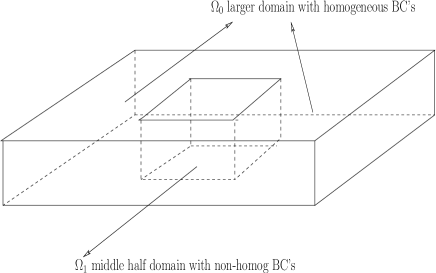
Figure 1: The larger domain $\mathcal{M}$ and the middle half domain $\mathcal{M}_{1}$

4.1 Simulation on the larger domain

In the simulation, the initial conditions are given for these scalar functions:

(4.1) $$\begin{cases}u(x,y,z,0)=\dfrac{x}{L_{1}}\dfrac{2\pi}{L_{2}}\sin{(\dfrac{2\pi x}{L_{1}})}\cos{(\dfrac{2\pi y}{L_{2}})}+\sin{(\dfrac{4\pi x}{L_{1}})}\cos{(\dfrac{4\pi y}{L_{2}})}\cos{(\dfrac{\pi z}{H})},\\ v(x,y,z,0)=\dfrac{-1}{L_{1}}\left(\sin{(\dfrac{2\pi x}{L_{1}})}+\dfrac{2\pi x}{L_{1}}\cos{(\dfrac{2\pi x}{L_{1}})}\right)\sin{(\dfrac{2\pi y}{L_{2}})}\\ \hskip 59.75095pt+\dfrac{L_{2}}{L_{1}}\left(\sin^{2}{(\dfrac{4\pi x}{L_{1}})}+\sin{(\dfrac{4\pi x}{L_{1}})}\sin{(\dfrac{4\pi y}{L_{2}})}\cos{(\dfrac{\pi z}{H})}\right),\\ w(x,y,z,0)=\dfrac{-4H}{L_{1}}(\sin{(\dfrac{4\pi x}{L_{1}})}+\cos{(\dfrac{4\pi x}{L_{1}})})\cos{(\dfrac{4\pi y}{L_{2}})}\sin{(\dfrac{\pi z}{H})},\\ \phi(x,y,z,0)=\bar{U}_{0}\sin{(\dfrac{2\pi x}{L_{1}})}\sin{(\dfrac{2\pi y}{L_{2}})}(\cos{(\dfrac{\pi z}{H})}-\cos{(\dfrac{2\pi z}{H})}),\\ \psi(x,y,z,0)=\dfrac{\pi\bar{U}_{0}}{H}\sin{(\dfrac{2\pi x}{L_{1}})}\sin{(\dfrac{2\pi y}{L_{2}})}(2\sin{(\dfrac{2\pi z}{H})}-\sin{(\dfrac{\pi z}{H})}).\end{cases}$$

We note here that these initial functions $u,v,w,\phi$, and $\psi$ satisfy the homogeneous boundary conditions for each mode $n\geq 0$. Specifically, for the zeroth mode, i.e. when $n=0$,

(4.2) $$\begin{cases}u_{0}(0,y,t)=0,\quad u_{0}(L_{1},y,t)=0,\\ v_{0}(0,y,t)=0,\quad v_{0}(x,0,t)=0,\quad v_{0}(x,L_{2},t)=0;\end{cases}$$

for the subcritical modes, i.e. when $1\leq n<n_{c}$,

(4.3) $$\begin{cases}\xi_{n}(0,y,t)=0,\quad v_{n}(0,y,t)=0,\quad\eta_{n}(L_{1},y,t)=0,\\ \alpha_{n}(x,L_{2},t)=0,\quad\beta_{n}(x,0,t)=0;\end{cases}$$

and for the supercritical modes, i.e. when $n>n_{c}$,

(4.4) $$\begin{cases}\xi_{n}(0,y,t)=0,\quad v_{n}(0,y,t)=0,\quad\eta_{n}(0,y,t)=0,\\ \alpha_{n}(x,L_{2},t)=0,\quad\beta_{n}(x,0,t)=0.\end{cases}$$

In this simulation, we take 400 segments in the $x$-direction, and 200 segments in the $y$ direction. When restricted to the middle half domain, the functions (4.1) also provide the initial conditions for the simulations on the middle half domain.

The simulation results over the larger domain $\mathcal{M}$ are plotted in Figures 2 to 17. Figure 2 is the cone plot with isosurface of the initial state of the velocity field, and Figures 3 and 4 are the slice–plane plots of the initial state of $\phi$ and $\psi$. Figures 5 to 9 are the contour plots of $u$, $v$, $w$, $\psi$ and $\phi$, respectively, on the plane $z=-2,500m$, at $t=0$.

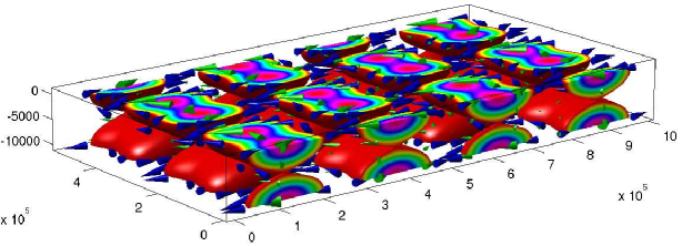
Figure 2: The initial state of velocity field in the larger domain $\mathcal{M}$

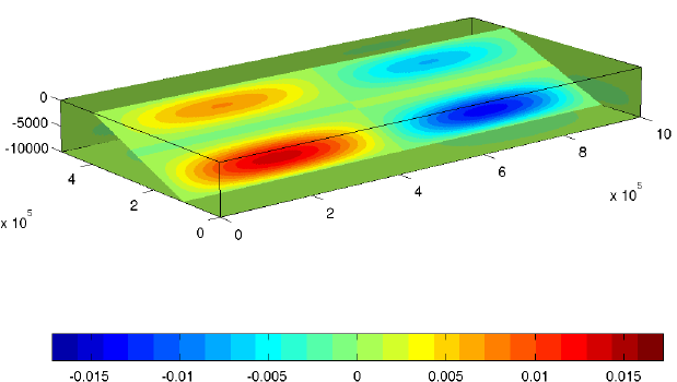
Figure 3: The initial state of $\psi$ in the larger domain $\mathcal{M}$

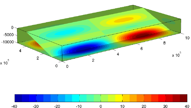
Figure 4: The initial state of $\phi$ in the larger domain $\mathcal{M}$

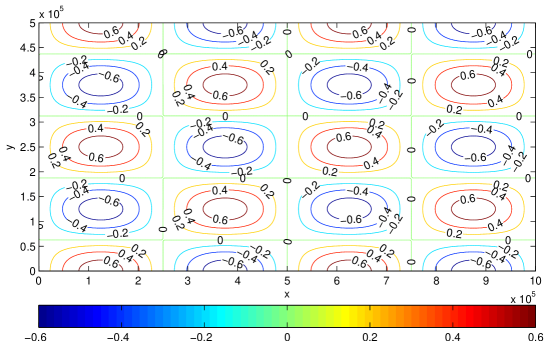
Figure 5: Contour plot of $u$ at $z=-2500m$, at $t=0$.

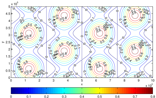
Figure 6: Contour plot of $v$ at $z=-2500m$, at $t=0$.

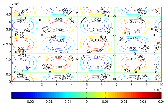
Figure 7: Contour plot of $w$ at $z=-2500m$, at $t=0$.

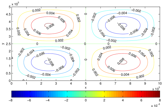
Figure 8: Contour plot of $\psi$ at $z=-2500m$, at $t=0$.

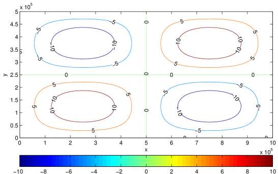
Figure 9: Contour plot of $\phi$ at $z=-2500m$, at $t=0$.

Figure 10 is the cone plot with isosurface of the velocity field at the final time $t=T$, and Figures 11 and 12 are the slice–plane plots of the state of $\phi$ and $\psi$ at the final time $t=T$. Figures 13 to 17 are the contour plots of $u$, $v$, $w$, $\psi$ and $\phi$, respectively, on the plane $z=-2,500m$, at $t=T$.

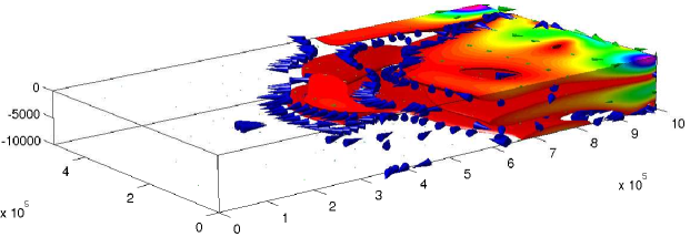
Figure 10: The velocity field with cone plot in the larger domain $\mathcal{M}$ at $t=T$

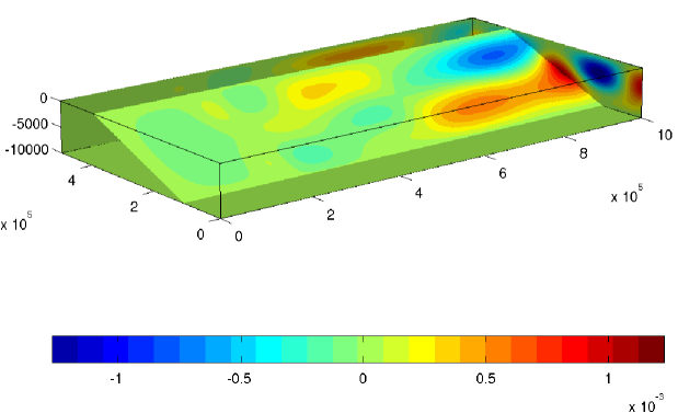
Figure 11: The state of $\psi$ in the larger domain $\mathcal{M}$ at $t=T$.

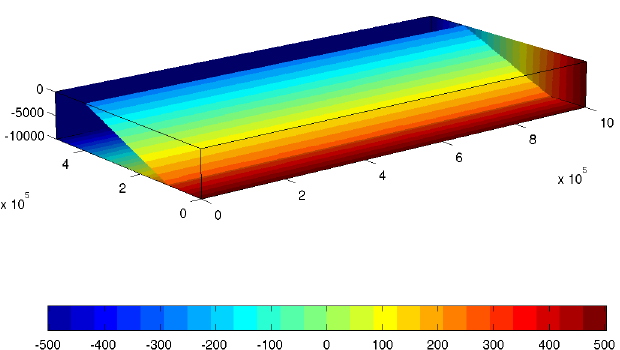
Figure 12: The state of $\phi$ in the larger domain $\mathcal{M}$ at $t=T$.

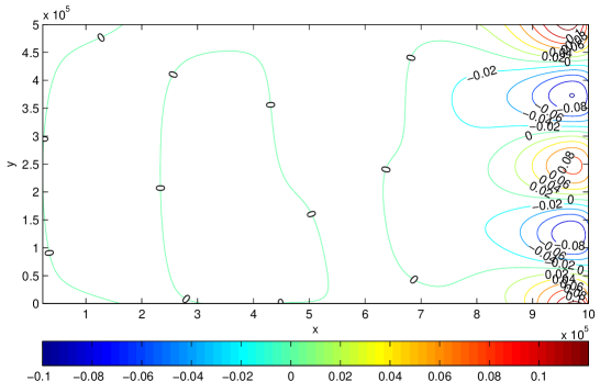
Figure 13: Contour plot of $u$ at $z=-2500m$, at $t=T$.

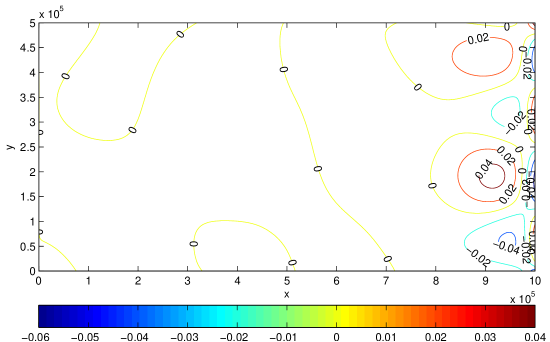
Figure 14: Contour plot of $v$ at $z=-2500m$, at $t=T$.

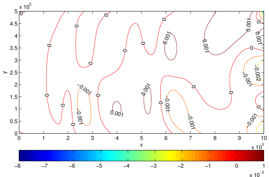
Figure 15: Contour plot of $w$ at $z=-2500m$, at $t=T$.

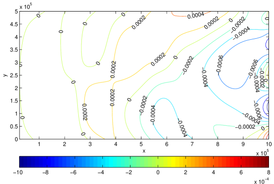
Figure 16: Contour plot of $\psi$ at $z=-2500m$, at $t=T$.

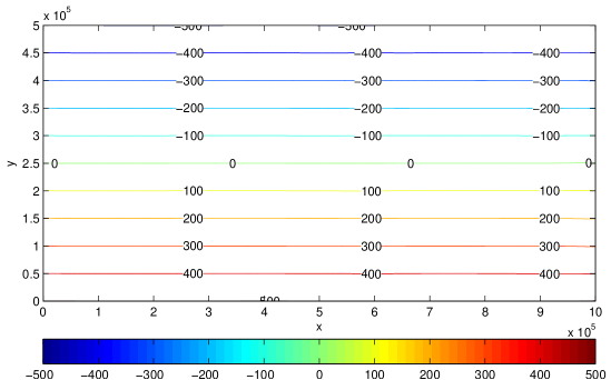
Figure 17: Contour plot of $\phi$ at $z=-2500m$, at $t=T$.

4.2 Simulation in the middle-half domain

As explained in the Introduction, we next do simulations on the middle half domain $\mathcal{M}_{1}$ of $\mathcal{M}$, $\mathcal{M}_{1}=\mathcal{M}_{1}^{\prime}\times(-H,0)$, $\mathcal{M}_{1}^{\prime}=(\frac{L_{1}}{4},\frac{3\,L_{1}}{4})\times(\frac{L_{2}}{4},\frac{3\,L_{2}}{4}).$ The boundary values of the unknown functions $u,\,v,\,w,\,\phi,$ and $\psi$ are inferred from the previous simulation. More specifically, the boundary conditions are, for the zeroth mode ($n=0$),

(4.5) $$\begin{cases}u_{0}(L_{1}/4,y_{j},t_{k})=u^{l}_{0}(L_{1}/4,y_{j},t_{k}),\\ u_{0}(3L_{1}/4,y_{j},t_{k})=u^{l}_{0}(3L_{1}/4,y_{j},t_{k}),\\ v_{0}(L_{1}/4,y_{j},t_{k})=v^{l}_{0}(L_{1}/4,y_{j},t_{k}),\\ v_{0}(x_{i},L_{2}/4,t_{k})=v^{l}_{0}(x_{i},L_{2}/4,t_{k}),\\ v_{0}(x_{i},3L_{2}/4,t_{k})=v^{l}_{0}(x_{i},3L_{2}/4,t_{k}).\end{cases}$$

For the subcritical modes ($1\leq n\leq n_{c}$),

(4.6) $$\begin{cases}\xi_{n}(L_{1}/4,y_{j},t_{k})=\xi^{l}_{n}(L_{1}/4,y_{j},t_{k}),\\ v_{n}(L_{1}/4,y_{j},t_{k})=v^{l}_{n}(L_{1}/4,y_{j},t_{k}),\\ \eta_{n}(3L_{1}/4,y_{j},t_{k})=\eta^{l}_{n}(3L_{1}/4,y_{j},t_{k}),\\ \alpha_{n}(x_{i},3L_{2}/4,t_{k})=\alpha^{l}_{n}(x_{i},3L_{2}/4,t_{k}),\\ \beta_{n}(x_{i},L_{2}/4,t_{k})=\beta^{l}_{n}(x_{i},L_{2}/4,t_{k}),\end{cases}$$

and for the supercritical modes ($n>n_{c}$),

(4.7) $$\begin{cases}\xi_{n}(L_{1}/4,y_{j},t_{k})=\xi^{l}_{n}(L_{1}/4,y_{j},t_{k}),\\ v_{n}(L_{1}/4,y_{j},t_{k})=v^{l}_{n}(L_{1}/4,y_{j},t_{k}),\\ \eta_{n}(L_{1}/4,y_{j},t_{k})=\eta^{l}_{n}(L_{1}/4,y_{j},t_{k}),\\ \alpha_{n}(x_{i},3L_{2}/4,t_{k})=\alpha^{l}_{n}(x_{i},3L_{2}/4,t_{k}),\\ \beta_{n}(x_{i},L_{2}/4,t_{k})=\beta^{l}_{n}(x_{i},L_{2}/4,t_{k}).\end{cases}$$

In the above, $x_{i}$, $y_{j}$ and $t_{k}$ denote the discrete grid points in space and time. The superscript $l$ denotes the previous simulation in the larger domain $\mathcal{M}$. In this simulation, we take 200 segments in the $x$-direction, and 100 segments in the $y$ direction.

The simulation results over the middle half domain $\mathcal{M}_{1}$ are plotted in Figures 18 to 25. Figure 18 is the cone plot with isosurface of the velocity field in the middle half domain $\mathcal{M}_{1}$ at the final time $t=T$, and Figures 19 and 20 are the slice–plane plots of the state of $\phi$ and $\psi$ in the middle half domain $\mathcal{M}_{1}$ at the final time $t=T$. Figures 21 and 25 are the contour plots of $u$, $v$, $w$, $\psi$ and $\phi$, respectively, on the plane $z=-2,500m$ restricted to the middle half domain $\mathcal{M}_{1}$, at $t=T$.

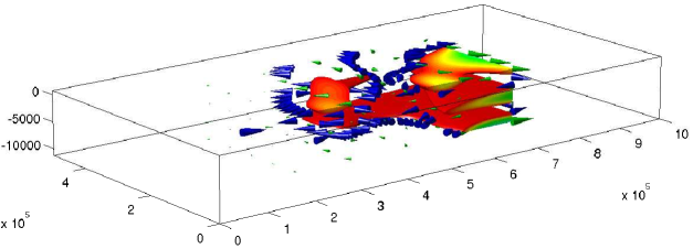
Figure 18: The velocity field with cone plot in the middle half domain $\mathcal{M}_{1}$ at $t=T$

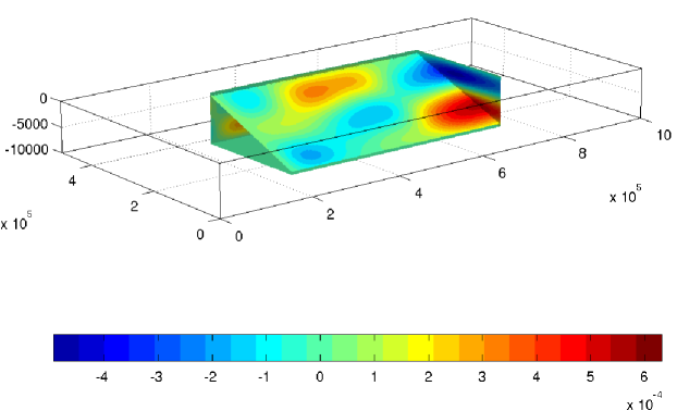
Figure 19: The state of $\psi$ in the middle half domain $\mathcal{M}_{1}$ at $t=T$.

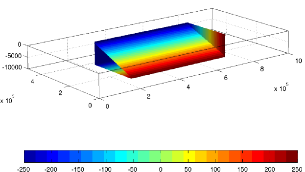
Figure 20: The state of $\phi$ in the middle half domain $\mathcal{M}_{1}$ at $t=T$.

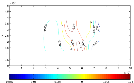
Figure 21: Contour plot of $u$ at $z=-2500m$, at $t=T$.

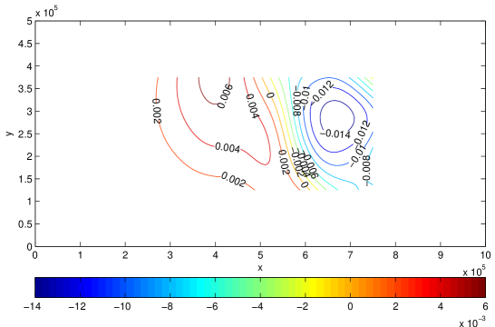
Figure 22: Contour plot of $v$ at $z=-2500m$, at $t=T$.

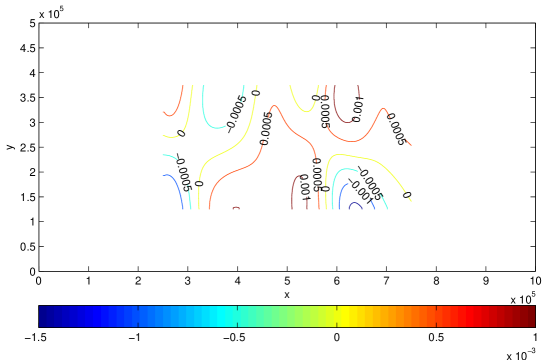
Figure 23: Contour plot of $w$ at $z=-2500m$, at $t=T$.

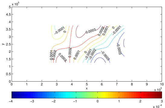
Figure 24: Contour plot of $\psi$ at $z=-2500m$, at $t=T$.

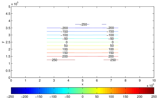
Figure 25: Contour plot of $\phi$ at $z=-2500m$, at $t=T$.

4.3 Comparison

In this subsection, we compare these two distinct simulations namely the results of the simulations on the larger domain $\mathcal{M}$ restricted to the middle half domain $\mathcal{M}_{1}$ and the results of the simulations on the middle half domain $\mathcal{M}_{1}$, as obtained by the second simulation above.

Let $u^{ext},\,v^{ext},\,w^{ext},\,\phi^{ext}$ and $\psi^{ext}$ be the numerical approximations of the variables $u,\,v,\,w,\,\phi$, and $\psi$ on the larger domain $\mathcal{M}$, respectively, and $u^{int},\,v^{int},\,w^{int},\,\phi^{int}$ and $\psi^{int}$ be the numerical approximations of the variables $u,\,v,\,w,\,\phi$, and $\psi$ on the middle half domain $\mathcal{M}_{1}$, respectively. In Figures 26-30, we plot the evolution of the unknowns, and of their relative errors (see below), in both the $L^{2}$ and $L^{\infty}$ norms. The relative errors are defined as $\dfrac{||u^{int}-u^{ext}|_{\mathcal{M}_{1}}||_{L^{p}}}{||u^{ext}||_{L^{p}}}$, etc. where $p=2,\infty$.

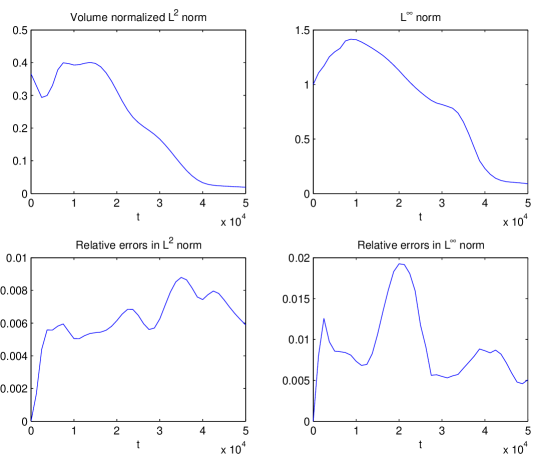
Figure 26: Top row: evolution of the solution $u$ in $L^{2}$ and $L^{\infty}$ norms. Bottom row: evolution of the relative errors for $u$ in $L^{2}$ and $L^{\infty}$ norms.

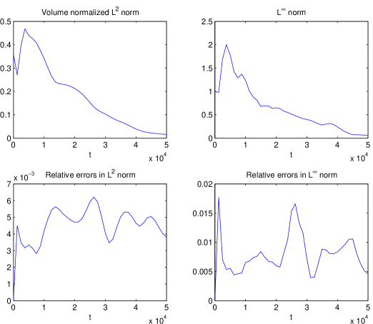
Figure 27: Top row: evolution of the solution $v$ in $L^{2}$ and $L^{\infty}$ norms. Bottom row: evolution of the relative errors for $v$ in $L^{2}$ and $L^{\infty}$ norms.

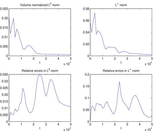
Figure 28: Top row: evolution of the solution $w$ in $L^{2}$ and $L^{\infty}$ norms. Bottom row: evolution of the relative errors for $w$ in $L^{2}$ and $L^{\infty}$ norms.

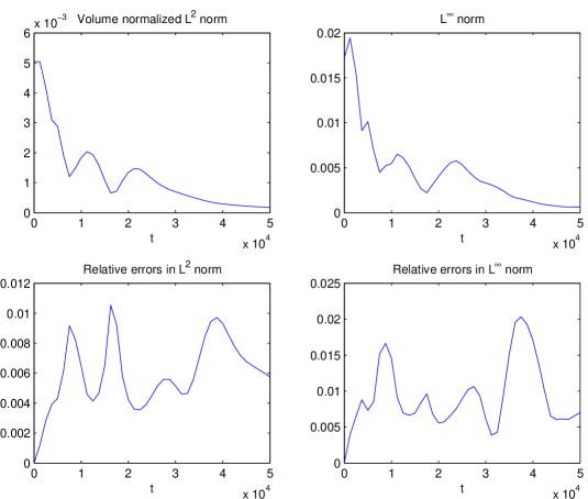
Figure 29: Top row: evolution of the solution $\psi$ in $L^{2}$ and $L^{\infty}$ norms. Bottom row: evolution of the relative errors for $\psi$ in $L^{2}$ and $L^{\infty}$ norms.

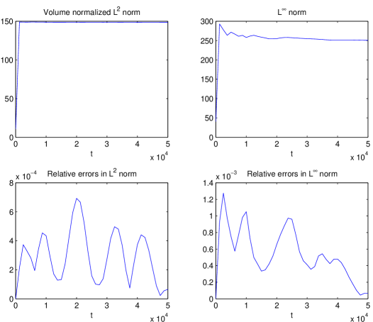
Figure 30: Top row: evolution of the solution $\phi$ in $L^{2}$ and $L^{\infty}$ norms. Bottom row: evolution of the relative errors for $\phi$ in $L^{2}$ and $L^{\infty}$ norms.

We observe that both the $L^{2}$ and the $L^{\infty}$ norms of the prognostic variables $u$, $v$ and $\psi$ are diminishing in time. This can be explained by the homogeneous boundary conditions imposed on the boundary of the larger domain $\mathcal{M}$ and by the fact that the velocity field is flowing out of the domain to the right, with a constant velocity $U_{0}$. The relative errors of the prognostic variables, in both the $L^{2}$ and the $L^{\infty}$ norms, are of the magnitude $O(10^{-2})$ or smaller, which means that results on the larger domain $\mathcal{M}$ and the results on the middle half domain $\mathcal{M}_{1}^{\prime}$ match very well.

For the diagnostic variables, the $L^{2}$ and the $L^{\infty}$ norms of $w$ are also diminishing in time, as for the prognostic variables; the relative errors for $w$ are large $\left(O(10^{-1})\right)$ as compared to those for the prognostic variables, but they are still well controlled. The bizarre behavior of the $L^{2}$ and the $L^{\infty}$ norms of $\phi$ can be explained by the absence of an evolution equation for $\phi$ and the lack of natural boundary conditions for $\phi_{0}$ in (3.3). The relative errors for $\phi$ are however very well controlled. Note that the relative errors for $u$, $v$, and $\psi$, in both the $L^{2}$ and $L^{\infty}$ norms, are of the order of $O(10^{-2})$, and the relative errors for $w$ are of the order of $O(10^{-1})$.

A graph of the absolute divergence averaged over the guest integration area is presented in Figure 31 for three cases: larger domain, the middle-half domain from direct computation, and the middle-half domain using the data from the larger domain. We observe that the mean absolute divergence for three cases are small and diminishing in time. This can be explained by the divergence free condition employed on the proposed numerical schemes. Furthermore, Figure 31 shows that the behaviors of the mean absolute divergence match well on the middle-half domain $\mathcal{M}_{1}$.

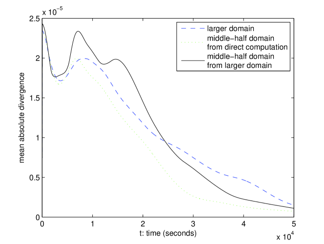
Figure 31: Evolution of the mean absolute divergence for three cases.

5 Conclusions

In conclusion, the absence of blowing up demonstrates that the boundary conditions proposed in Section 2.2 are suitable for the problem, and the numerical scheme proposed in Section 3 is stable. The fact that the numerical results match very well on the middle half domain $\mathcal{M}_{1}$ demonstrates the transparency property of the boundary conditions.

From the results of this idealized model it is straightforward to outline the algorithmic path to be taken in the application of this method to the full primitive equations. The simplest approach would be first to re-write the model equations so that they are formally equivalent to the system (2.1). This involves specifying a reasonable, local mean stratification $N^{2}$, and mean zonal wind, $\bar{U}_{0}$.

Next a vertical mode decomposition is performed to identify the subcritical/supercritical mode division. Next, the appropriate lateral boundary conditions are applied. Lastly the modal decomposition is summed to reconstruct the boundary values of the field variables. As necessary, the local mean stratification and zonal wind can be adjusted.

This would be superior to methods that absorb wave energy through nudging since the artificial damping also inevitably causes the interior solution to decay and the sponge layer, itself, induces wave reflection.

References

- [1] C. Cao and E. S. Titi, Global well-posedness of the three-dimensional viscous primitive equations of large scale ocean and atmosphere dynamics, Ann. of Math. (2), 166 (2007), pp. 245–267.
- [2] Q. Chen, J. Laminie, A. Rousseau, R. Temam, and J. Tribbia, A 2.5D model for the equations of the ocean and the atmosphere, Anal. Appl. (Singap.), 5 (2007), pp. 199–229.
- [3] Q. Chen, M.-C. Shiue, and R. Temam, The barotropic mode for the primitive equations, Journal of Scientific Computing, 45 (2010), pp. 167–199.
- [4] Q. Chen, R. Temam, and J. J. Tribbia, Simulations of the 2.5D inviscid primitive equations in a limited domain, J. Comput. Phys., 227 (2008), pp. 9865–9884.
- [5] A. Chorin, Numerical solution of the Navier-Stokes equations, Math. Comp., 22 (1968), pp. 745–762.
- [6] B. Engquist and A. Majda, Absorbing boundary conditions for the numerical simulation of waves, Math. Comp., 31 (1977), pp. 629–651.
- [7] D. Givoli and B. Neta, High-order nonreflecting boundary conditions for the dispersive shallow water equations, J. Comput. Appl. Math., 158 (2003), pp. 49–60. Selected papers from the Conference on Computational and Mathematical Methods for Science and Engineering (Alicante, 2002).
- [8] J. Guermond, P. Minev, and J. Shen, An overview of projection methods for incompressible flow, Comput. Methods Appl. Mech. Engrg, Vol. 195 (2006), pp. 6011–6045.
- [9] R. L. Higdon, Absorbing boundary conditions for difference approximations to the multidimensional wave equation, Math. Comp., 47 (1986), pp. 437–459.
- [10] G. Kobelkov, Existence of a solution ‘in the large’ for the 3D large-scale ocean dynamics equations, C. R. Math. Acad. Sci. Paris, 343 (2006), pp. 283–286.
- [11] G. M. Kobelkov, Existence of a solution “in the large” for ocean dynamics equations, J. Math. Fluid Mech., 9 (2007), pp. 588–610.
- [12] J. Lions, R. Temam, and S. Wang, New formulations of the primitive equations of atmosphere and applications, Nonlinearity, 5 (1992), pp. 237–288.
- [13] , On the equations of the large-scale ocean, Nonlinearity, 5 (1992), pp. 1007–1053.
- [14] G. Marchuk, Methods and problems of computational mathematics, Actes du Congres International des Mathematiciens(Nice, 1970), 1 (1971), pp. 151–161.
- [15] M. Marion and R. Temam, Navier-Stokes equations: theory and approximation, in Handbook of numerical analysis, Vol. VI, Handb. Numer. Anal., VI, North-Holland, Amsterdam, 1998, pp. 503–688.
- [16] A. McDonald, Transparent boundary conditions for the shallow water equations: testing in a nested environment, Mon. Wea. Rev., 131 (2003), pp. 698–705.
- [17] I. M. Navon, B. Neta, and M. Y. Hussaini, A perfectly matched layer approach to the linearized shallow water equations models, Monthly Weather Review, 132 (2004), pp. 1369–1378.
- [18] J. Oliger and A. Sundström, Theoretical and practical aspects of some initial boundary value problems in fluid dynamics, SIAM J. Appl. Math., 35 (1978), pp. 419–446.
- [19] J. Pedlosky, Geophysical fluid dynamics, 2nd edition, Springer, 1987.
- [20] M. Petcu, R. Temam, and M. Ziane, Mathematical problems for the primitive equations with viscosity, in Handbook of Numerical Analysis. Special Issue on Some Mathematical Problems in Geophysical Fluid Dynamics, R. T. P.G. Ciarlet EDs and J. T. G. Eds, eds., Handb. Numer. Anal., Elsevier, New York, 2008.
- [21] A. Rousseau, R. Temam, and J. Tribbia, Boundary conditions for the 2D linearized PEs of the ocean in the absence of viscosity, Discrete Contin. Dyn. Syst., 13 (2005), pp. 1257–1276.
- [22] , Numerical simulations of the inviscid primitive equations in a limited domain, in Analysis and Simulation of Fluid Dynamics, Advances in Mathematical Fluid Mechanics, Caterina Calgaro and Jean-François Coulombel and Thierry Goudon, 2007.
- [23] , The 3D primitive equations in the absence of viscosity: boundary conditions and well-posedness in the linearized case, J. Math. Pures Appl. (9), 89 (2008), pp. 297–319.
- [24] A. Rousseau, R. Temam, and J. Tribbia, Boundary value problems for the inviscid primitive equations in limited domains, in Computational Methods for the Oceans and the Atmosphere, Special Volume of the Handbook of Numerical Analysis, P. G. Ciarlet, Ed, R. Temam and J. Tribbia, Guest Eds, Elesevier, Amsterdam, (2009).
- [25] R. Temam, Sur l’approximation de la solution des équations de Navier-Stokes par la méthode des pas frationnaires (ii), Arch. Rational Mech. Anal., 33 (1969), pp. 377–385.
- [26] R. Temam and J. Tribbia, Open boundary conditions for the primitive and Boussinesq equations, J. Atmospheric Sci., 60 (2003), pp. 2647–2660.
- [27] R. Temam and M. Ziane, Some mathematical problems in geophysical fluid dynamics, in Handbook of mathematical fluid dynamics, S. Friedlander and D. Serre, eds., North-Holland, 2004.
- [28] J. van Kan, A second-order accurate pressure-correction scheme for viscous incompressible flow, SIAM J. Sci. Statist. Comput., 7 (1986), pp. 870–891.
- [29] T. Warner, R. Peterson, and R. Treadon, A tutorial on lateral boundary conditions as a basic and potentially serious limitation to regional numerical weather prediction, Bull. Amer. Meteor. Soc., 78 (1997), pp. 2599–2617.
- [30] W. Washington and C. Parkinson, An introduction to three-dimensional climate modelling, Univ. Sci. Books, Sausalito, CA, 2nd ed., 2005.
- [31] N. Yanenko, The method of fractional steps. The solution of problems of mathematical physics in several variables, Springer-Verlag, 1971. English translation.