SCUBA-2 Data Processing

Abstract

SCUBA-2 is the largest submillimetre array camera in the world and was commissioned on the James Clerk Maxwell Telescope (JCMT) with two arrays towards the end of 2009. A period of shared-risks observing was then completed and the full planned complement of 8 arrays, 4 at 850 $\mu$m and 4 at 450 $\mu$m, are now installed and ready to be commissioned. SCUBA-2 has 10,240 bolometers, corresponding to a data rate of 8 MB/s when sampled at the nominal rate of 200 Hz. The pipeline produces useful maps in near real time at the telescope and often publication quality maps in the JCMT Science Archive (JSA) hosted at the Canadian Astronomy Data Centre (CADC).

1 SMURF Iterative Map-Maker

The Sub-Millimetre Common-User Bolometer Array 2 (SCUBA-2) (Craig et al. (2010); Holland et al. (2006)) is a direct-detection bolometer array and so measures the temperature variation of the sky as well as the astronomical signal. Data are taken by scanning the telescope over the source using a pattern designed such that the time taken to return to the same place on the sky is not a fixed interval. The telescope software has been modified to use a number of different patterns called “pong”, “lissajous” and “daisy” that have this property (Kackley et al. (2010)). This allows the map-maker to separate time-varying signals from those that are fixed in a particular location on the sky. We have developed the SMURF software package (Sub-Millimetre User Reduction Facility; Chapin et al. (2010)) to process SCUBA-2 data. The SMURF map-maker works by iteratively fitting a collection of models to the time stream in turn, and subtracting them, leaving the astronomical signal. All model components are refined at each iteration, resulting in improved astronomical image estimates. However, before the iterations may begin, we must repair several problems with the bolometer time series. For example, the SQUID readout electronics can introduce steps which need to be fixed. We have developed a robust algorithm for correcting these problems and an example is shown in Fig. 1.

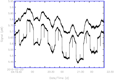
Figure 1.: The lower curve shows some flatfielded data containing many steps along with some spikes. The upper curve is the same data with the steps and spikes removed (including an offset of 0.15 pW to make this easier to see).

1.1 Data Models

After glitch repair, the time series data in Fig. 1 still have a periodic structure that is dominated by a 25 second oscillation in the fridge along with low-frequency variations due to changes in the sky power and instrument drifts. These signals are common to all the bolometers and so can be removed, albeit with a loss of sensitivity to signals larger than the array footprint. We reject any bolometers that do not exhibit this strong common-mode signal. In addition, the relative amplitudes of the common-mode in different bolometers may be used to refine the flatfield.

Other models include a Fourier filter to remove low and high frequencies from the data based on the scan speed of the telescope and the wavelength, correction for atmospheric extinction, and an alternative to the Fourier filter that removes a median value from a rolling box.

At the end of each iteration, once the low-frequency noise and astronomical signal components have been estimated and removed, the residual signal is considerably flatter making it easy to identify smaller spikes. We have also implemented a map-based despiker that identifies outliers in the data that land in each map pixel. This procedure is repeated until the RMS of the residuals do not change appreciably. Fig. 2 shows an example of some models for a source in the Orion Molecular Cloud and Fig. 3 shows a commissioning observation compared with some commissioning data from the first SCUBA taken in 1997.

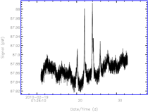
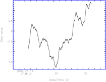
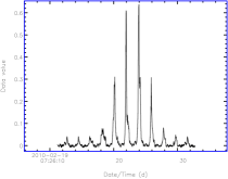
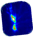
Figure 2.: Top left shows some raw flatfielded time-series data from a single bolometer for a 20 second observation of a source in Orion. Top right is the common-mode signal and the bottom left is the astronomical signal determined from the time series after removing all the models. The final map is shown bottom right and covers an area of about 4 arcmin $\times$ 4 arcmin.

2 Pipeline and the JCMT Science Archive

At the telescope and at the JSA (hosted at CADC) we use the ORAC-DR data reduction pipeline (Cavanagh et al. (2008)) to run the SMURF map-maker and to perform mosaicking, pointing corrections and data analysis. PiCARD (Jenness et al. (2008)) is used for off-line data analysis.

At the summit there are two pipelines, one for each wavelength, for Quick Look, and two pipelines for science processing all running on dedicated machines. The Quick Look pipeline (Gibb et al. (2005)) processes single observations as quickly as possible to provide instant feedback to the observer and also to reduce pointing and focus observations. The science pipelines have a little more time to process the data and can demonstrate observation progress by waiting for more data to accumulate and mosaicking multiple observations.

In the JSA time is not an issue, so the pipeline can run on the CADC grid processing cloud (Economou et al. (2011)) using more complex models and many more iterations. It is also possible to run the pipeline in the new CANFAR cloud computing infrastructure (Gaudet et al. (2011)).

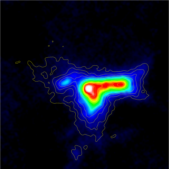
Figure 3.: Commissioning image of IRAS 18592+0108 at 450 $\mu$m taken on 2009 October 25th with contours from an 850 $\mu$m SCUBA scan map commissioning observation from 1997 August 19th (see also Gear et al. (1996)).

References

- Cavanagh et al. (2008) Cavanagh, B., Jenness, T., Economou, F., & Currie, M. J. 2008, Astronomische Nachrichten, 329, 295
- Chapin et al. (2010) Chapin, E., Gibb, A. G., Jenness, T., Berry, D. S., & Scott, D. 2010, Starlink User Note 258, Joint Astronomy Centre
- Craig et al. (2010) Craig, S. C., et al. 2010, in Society of Photo-Optical Instrumentation Engineers (SPIE) Conference Series, vol. 7741
- Economou et al. (2011) Economou, F., et al. 2011, in ADASS XX, edited by I. N. Evans, A. Accomazzi, D. J. Mink, & A. H. Rots (San Francisco: ASP), vol. TBD of ASP Conf. Ser., TBD
- Gaudet et al. (2011) Gaudet, S., et al. 2011, in ADASS XX, edited by I. N. Evans, A. Accomazzi, D. J. Mink, & A. H. Rots (San Francisco: ASP), vol. TBD of ASP Conf. Ser., TBD
- Gear et al. (1996) Gear, W. K., Holland, W. S., Cunningham, C. R., & Lightfoot, J. F. 1996, in Submillimetre and Far-Infrared Space Instrumentation, edited by E. J. Rolfe & G. Pilbratt, vol. 388 of ESA Special Publication, 135
- Gibb et al. (2005) Gibb, A. G., Scott, D., Jenness, T., Economou, F., Kelly, B. D., & Holland, W. S. 2005, in Astronomical Data Analysis Software and Systems XIV, edited by P. Shopbell, M. Britton, & R. Ebert, vol. 347 of Astronomical Society of the Pacific Conference Series, 585
- Holland et al. (2006) Holland, W., et al. 2006, in Society of Photo-Optical Instrumentation Engineers (SPIE) Conference Series, vol. 6275
- Jenness et al. (2008) Jenness, T., Cavanagh, B., Economou, F., & Berry, D. S. 2008, in Astronomical Data Analysis Software and Systems XVII, edited by R. W. Argyle, P. S. Bunclark, & J. R. Lewis, vol. 394 of Astronomical Society of the Pacific Conference Series, 565
- Kackley et al. (2010) Kackley, R., Scott, D., Chapin, E., & Friberg, P. 2010, in Society of Photo-Optical Instrumentation Engineers (SPIE) Conference Series, vol. 7740