TIFR/TH/10-34

Axions as Quintessence in String Theory

Sudhakar Panda¹, Yoske Sumitomo², and Sandip P. Trivedi²

¹ Harish-Chandra Research Institute, Allahabad 211019, India

² Tata Institute of Fundamental Research, Mumbai 400005, India

Email: panda@mri.ernet.in, sumitomo@theory.tifr.res.in, trivedi.sp@gmail.com

1 Introduction

Observational evidence shows that the universe is accelerating and therefore must be dominated, at cosmological scales, by a mysterious form of energy called Dark Energy. Understanding its nature is a central challenge that faces us today. The leading candidate for dark energy is the cosmological constant. It is consistent with observations. Theoretically, we now know that a positive cosmological constant can arise from a consistent theory of quantum gravity like string theory and this gives us greater confidence in the idea being correct.

Another possibility for dark energy is quintessence, see [2, 3, 4, 5, 6] for reviews. In this case the vacuum energy is not a constant but instead slowly relaxes due to the evolution of a scalar field. This makes the resulting equation of state for dark energy time dependent. Observations in the coming decade will attempt to determine the equation of state of dark energy and, hopefully will allow us to decide between these possibilities.

In this paper we will construct a model of quintessence in string theory. One can view this as a sort of “theoretical test” of this idea. If the idea fits in with string theory one would have greater confidence in it, just as for the cosmological constant. One can also hope that such constructions might ultimately lead to some interesting constraints which can then be tested observationally.

The idea behind quintessence is quite similar to that in inflation. However, an important difference, which makes the construction of models of quintessence considerably more challenging, is that the energy scale for quintessence is of order

$$\Lambda\sim 10^{-3}\,{\rm eV}$$ (1.1)

and therefore is much smaller than the scale of supersymmetry breaking. This leads to two important issues which any model of quintessence must confront. The first is to ensure that the potential for the quintessence field has a scale of order $\Lambda$ and not of order the SUSY breaking scale; this issue is related to the cosmological constant problem. The second is to have a potential for the quintessence field which meets the slow-roll conditions despite the relatively high scale of supersymmetry breaking. In particular this requires that the mass of the quintessence field is of order the Hubble constant today, $H\sim 10^{-33}\,{\rm eV}$, and therefore is much smaller than the SUSY breaking scale, which must be at least $M_{SB}\sim 1-10\,{\rm TeV}$ and typically is much higher . Now, it is a famous fact, responsible for the hierarchy problem in the standard model, that scalar fields tend to have their mass driven up to the SUSY breaking scale. Ensuring that the quintessence field has a mass $m\sim H$ so that the ratio ${m/M_{SB}}$ is at least $10^{-45}$ if not smaller is therefore not easy.

In this paper we will, to begin, ignore the first question, related to the cosmological constant question, and focus on the construction of a model which meets the second challenge of ensuring that the slow-roll conditions are met despite the high scale of SUSY breaking. We will return to a discussion of the cosmological constant question in §6. Within the context of a model of the type we construct, we will argue that anthropic considerations could well result in the energy density in dark energy being shared between the cosmological constant and the quintessence field in a reasonably equitable fashion. As a result an evolving equation of state might well be more natural from the point of view of anthropic considerations in such a model.

Before proceeding it is useful to phrase the requirement for a small mass for the quintessence field in terms of restrictions on higher dimensional operators in the low-energy effective field theory. Taking $M_{SB}\sim 1\,{\rm TeV}$, and the mass $m\sim H$, one finds that for the current value of $H\sim 10^{-33}\,{\rm eV},$

$$m^{2}\sim H^{2}\sim{M_{SB}^{8}\over M_{Pl}^{6}}.$$ (1.2)

This shows that upto dimension $10$ operators which could contribute to the mass have to be suppressed to construct a satisfactory model. For a higher scale of SUSY breaking the suppression would have to be even more severe. The requirements of slow-roll are therefore indeed quite restrictive . This estimate also illustrates why the construction of a quintessence model is sensitive to Planck scale physics and can therefore be sensibly carried out only within a UV complete theory of gravity such as string theory. In fact in the model we construct the canonically normalized quintessence field typically undergoes an excursion of order the Planck scale in the course of its evolution and the potential needs to be flat for this whole range in field space. Needless to say, ensuring this while working only in an effective field theory would be extremely difficult.

Qualitatively, there are two possibilities within string theory for a quintessence field [7]. It could be a modulus like the dilaton or the overall volume which runs off to infinity in field space. In such a situation the coupling constants of the standard model, like the fine structure constant or the four dim. gravitational constant, would also vary with time and one would also need to ensure that this variation is small enough. Such models would be observationally very interesting but are quite challenging to construct. Instead, we will opt here for a second possibility which seems easier to implement. In our case the field will be an axion, which is a sort of Goldstone boson, that runs to a finite point in field space where its potential is minimized. We will take this finite point to be at the origin.

It is well known that axion fields often arise in string compactifications. In our construction, which is in IIB string theory, the axion of interest will arise from the RR sector. A general argument then ensures that there is a shift symmetry, under which the axion shifts by a constant, which is unbroken to all orders in the quantum loop expansion. This feature will be very helpful in ensuring that the resulting potential is varying slowly enough and can be isolated from the effects of supersymmetry breaking.

The shift symmetry will have to be broken of course, at some level, to generate a potential for the axion. A natural possibility to consider is that the breaking arises from non-perturbative effects like instantons. It turns out though that this does not lead to an acceptable model for quintessence . In this case the resulting potential is a periodic function of the axion. The slow-roll conditions then require the axion to have a decay constant of order the Planck scale or higher whereas requiring the energy density in the axion to be of the right magnitude gives an axion decay constant about two orders of magnitude smaller than the Planck scale [9, 8].

One therefore needs to explore other ways to break the shift symmetry. It turns out that the shift symmetry can also be broken in the presence of branes . By placing these branes in highly warped regions of the compactification one can make this breaking small . This idea is referred to as “axion monodromy”, and was developed in [10, 1, 11] to construct a model of chaotic inflation. The resulting potential one gets in this case is no longer periodic, in fact it is approximately linear in the axion . As a result, we will find that the slow-roll conditions and other requirements for quintessence can be met even with an axion whose decay constant is smaller than the Planck scale.

Following [1] (see also [11]), we will add a pair of NS5-brane and $\overline{\rm NS5}$-brane in highly warped regions of the compactification to break the axion shift symmetry. The axion, which is the zero mode of the RR two-form $C_{2}$ that arises due to a non-trivial two-cycle $\Sigma$, induces a D3-brane charge on the 5-brane which wraps the two-cycle $\Sigma$. It also induces $\overline{\mathrm{D}3}$-brane charge on the anti 5-brane . This results in additional 3-brane tension being induced on both the 5 and anti 5-branes which depends on the axion. The resulting potential turns out to be linear in the axion, for large enough values of this field.

To examine the effects of SUSY breaking and moduli stabilization on the axion potential we will consider the model of KKLT [12]. We will find that an additional important contribution to the axion potential does arise from these effects. The axion affects the warp factor of the geometry and this in turn changes the volume of the internal space. Once the volume is stabilized this gives rise to an extra potential for the axion. The leading contribution of this type would in fact be unacceptably big, but this can cancel exactly between the 5-brane and the anti 5-brane which induce opposite 3-brane charge, provided the two throats where they are located are related by a ${\mathbb{Z}}_{2}$ symmetry.

The subleading correction to the axion potential which survives cannot be calculated exactly, given our present understanding of flux compactifications, but an estimate which is adequate for the purposes of our discussion can be made following the discussion in [13, 14, 15]. This estimate tells us that the subleading effect is still important enough to be the dominant contribution to the axion potential, but it too is suppressed by the warp factor at the bottom of the throats where the 5-branes are located . By making this warp factor small enough one then finds that a satisfactory model of quintessence can indeed be constructed.

The bottom-line then is that a workable model for quintessence in string theory, based on the idea of axion monodromy, can be constructed by placing a 5-brane and anti 5-brane pair in highly warped throats in the presence of an axion. When the canonically normalized axion field has a expectation value which is of order the Planck scale, the slow-roll conditions are met, and the quintessence field evolves with an equation of state which can deviate significantly from that for the cosmological constant.

This paper is structured as follows. Some general considerations for models based on a non-perturbative potential and a linear potential are discussed in §2. The quintessence model we construct is then discussed in greater detail in §3. Additional terms which can arise once the dynamics of moduli stabilization is included are discussed in §4. §5 contains a more complete look at the final model including all important terms in the potential, and discusses the resulting energy scales in more detail. Some general features of the model are discussed in §6. These include the many very light particles which arise due to the highly warped throats in which the 5-branes are placed, the absence of tracker behavior and its relation to the cosmological constant issue, and a potentially interesting signal due to the rotation of the E mode of the CMB into the B mode. We end with conclusions in §7.

Let us end this introduction by commenting on some additional papers of relevance. A model of quintessence based on a linear potential was considered in [16], and was explored further in [17, 18] . The idea that quintessence might arise from many axion due to the effects of flux induced mixing was explored in [19]. The possibility of many light axions and the constraints that can be placed on them was discussed in [20, 21]. Finally [22], which appeared recently, discusses how additional fields can lead to flattened potentials.

2 Axions: General Considerations

The possibility of using an axion in string theory as the quintessence field, with the shift symmetry being broken by non-perturbative effects, has been considered in the past and has some well known difficulties. We begin by reviewing this case first.

Consider a canonically normalized axion field $\phi$ with action,

$$S=\int d^{4}x\sqrt{-g}\left[-{1\over 2}(\partial\phi)^{2}+V\left(\phi\over f_{a}\right)\right].$$ (2.1)

The axion potential in this case is a periodic function with a period of order $f_{a}$ - the axion decay constant. For example, a typical form for the potential is

$$V=\mu^{4}\cos\left({\phi\over f_{a}}\right),$$ (2.2)

where the scale $\mu^{4}$ goes like,

$$\mu^{4}\propto e^{-c\,S_{\rm inst}},$$ (2.3)

with $S_{\rm inst}$ being the action of the instanton which gives rise to the potential, and $c$ being a constant of order unity.

For the axion field to play the role of quintessence its potential must be slowly varying on cosmological scales and therefore should meet the well-known slow roll conditions. This gives rise to the requirements that

$${V^{\prime\prime}\over V}M_{Pl}^{2}\lesssim 1,\\ \left({V^{\prime}\over V}\right)^{2}M_{Pl}^{2}\lesssim 1.$$ (2.4)

For a periodic potential, e.g., of form eq.(2.2), it is easy to see that $V^{\prime\prime}/V\sim({V^{\prime}/V})^{2}\sim 1/f_{a}^{2}$. So the slow-roll conditions give the constraint

$$f_{a}\gtrsim M_{Pl}.$$ (2.5)

Now axions which arise in string theory typically satisfy the condition, [23, 24, 9, 8],

$$f_{a}\leq{M_{Pl}\over S_{\rm inst}},$$ (2.6)

where $S_{\rm inst}$ is the action of the instanton which gives rise to the axion potential.

For the axion potential $V$ in eq.(2.2), with eq.(2.3), to be of order $\Lambda^{4}$, eq.(1.1), requires an action, [8],

$$S_{\rm inst}\sim 200-300.$$ (2.7)

Thus we see that string constructions lead to an axion decay constant $f_{a}$, eq.(2.6), which is about two orders of magnitude smaller than the value required by the slow-roll conditions eq.(2.5).

With $N$ axions evolving together the mismatch does improve. The slow-roll conditions now lead to

$$f_{a}^{2}>{M_{Pl}^{2}\over N}.$$ (2.8)

However, agreement with eq.(2.6), eq.(2.7), requires, [8],

$$N\gtrsim 10^{4}-10^{5},$$ (2.9)

which is a large number indeed.

In the kind of construction we explore, the key new element is that the resulting axion potential is not a periodic function. Instead it is approximately a linear function of the axion [1]. The potential we get has the form

$$V(\phi)=\mu^{4}a={\mu^{4}\over f_{a}}\phi,$$ (2.10)

where $\mu$ is a mass scale and we have expressed the canonically normalized field $\phi$ in terms of the dimensionless axion $a$ as

$$\phi=f_{a}a.$$ (2.11)

The resulting action relevant for the late time evolution of the universe in our model is then

$$S_{axion}=\int d^{4}x\sqrt{-g}\left[M_{Pl}^{2}R-{1\over 2}f_{a}^{2}(\partial a)^{2}-\mu^{4}a\right].$$ (2.12)

For the potential eq.(2.10) the slow roll conditions eq.(2.4) give,

$$\phi>M_{Pl}.$$ (2.13)

In terms of the dimensionless axion $a$ this condition is,

$$a>{M_{Pl}\over f_{a}}.$$ (2.14)

The second condition we must impose is that the potential energy in the axion today is of order the total energy density in the universe,

$$\mu^{4}a\sim\Lambda^{4}\sim 10^{-12}\,({\rm eV})^{4}$$ (2.15)

From eq.(2.14) this gives rise to a condition on the scale of the potential $\mu$,

$$\mu^{4}\lesssim{f_{a}\over M_{Pl}}\Lambda^{4}.$$ (2.16)

These are in fact the only two important conditions that need to be imposed. As long as a model can be constructed with a linear potential, with a scale $\mu$ which meets the condition eq.(2.16), and in which the axion around the current epoch of the universe meets the condition in eq.(2.14), one would have a workable model of quintessence. Note in particular, that the slow-roll conditions, eq.(2.14), can be met in this model even when $f_{a}\leq M_{Pl}$ by choosing a large enough value of the axion.

Some additional points are also worth making at this stage.

First, the rolling axion gives rise to a stress energy of the perfect fluid form with an equation of state,

$$p=\omega_{a}\rho$$ (2.17)

where

$$\omega_{a}={{\dot{\phi}^{2}/2}-V\over{\dot{\phi}^{2}/2}+V}\sim{\epsilon/3-1\over\epsilon/3+1}$$ (2.18)

where $\epsilon$ is the slow roll parameter,

$$\epsilon={M_{Pl}^{2}\over 2}\left({V^{\prime}\over V}\right)^{2}={M_{Pl}^{2}\over 2\phi^{2}}.$$ (2.19)

When $\phi\sim O(M_{Pl})$ we see that $\omega_{a}$ can be significantly different from $-1$, the value for the equation of state of the cosmological constant.

Second, the value obtained for the equation of state parameter (from WMAP+BAO+$H_{0}$ + $D_{\Delta t}$ +SN) in [25] is

$$\omega_{\rm DE}(z)=w_{0}+w_{1}{z\over 1+z},\quad\omega_{0}=-0.93\pm 0.13,\quad\omega_{1}=-0.41^{+0.72}_{-0.71}.$$ (2.20)

Fitting to the central value in our model leads to the value,

$$\phi\sim 2.14M_{Pl}.$$ (2.21)

The time-dependent constraint $\omega_{1}$ is also satisfied.

Third, the axion satisfies the equation

$$\ddot{\phi}+3H\dot{\phi}+V^{\prime}=0.$$ (2.22)

When the slow roll conditions are satisfied,

$$3H\dot{\phi}+V^{\prime}=0,$$ (2.23)

the total change in the axion field during the evolution of the universe, upto the current epoch, can be estimated as

$$\delta\phi\sim\dot{\phi}H^{-1}\sim{V^{\prime}\over V}M_{Pl}^{2}\sim{M_{Pl}^{2}\over\phi}.$$ (2.24)

For $\phi$ of order the Planck scale we see that the total change in the axion during the evolution of the universe is also of order the Planck scale.

For a workable model, the potential must be slowly varying for this entire range of variation of the axion field. In particular, in our case the linear approximation with a slow enough rate of variation, should be valid for the entire range of evolution of the axion. This is a significant constraint to meet. As was discussed in the introduction it would be difficult to ensure this while working within a low-energy effective field theory alone. For once the axion shift symmetry is broken one would expect quadratic and higher terms to typically appear

$$V={\mu^{4}\over f_{a}}\phi+m^{2}\phi^{2}+\cdots{\phi^{n+4}\over M_{Pl}^{n}}$$ (2.25)

thereby ruining the flatness conditions required for slow-roll behavior. By embedding this construction in string theory we can go beyond general field theory considerations though and as we discuss below, we will find that in some models these corrections do not arise and the potential remains of linear form, with small corrections, for the entire range of $O(M_{Pl})$ variation in the canonically normalized axion.

3 More Details on the Model

We now turn to a more detailed description of the model.

We will work with flux compactifications in IIB string theory. This is a reasonably well studied corner of string theory by now, e.g, see [26, 27]. One starts with a Calabi-Yau manifold and carries out a suitable orientifolding to allow for the presence of flux. Then turning on flux and/or adding branes gives rise to a warped Calabi-Yau internal space.

The axion field we will consider arises in this setup from the zero-mode of a two-form field. There are two-possibilities, the NS two-form, $B_{2}$, or the RR two-form $C_{2}$. In the $C_{2}$ case we start with the ten-dim. action,

$$S={1\over(2\pi)^{7}\alpha^{\prime 4}}\int d^{10}x\sqrt{-g}\left[{1\over g_{s}^{2}}R-{1\over 12}\partial_{\mu}C_{ab}\partial^{\mu}C_{a^{\prime}b^{\prime}}g^{aa^{\prime}}g^{bb^{\prime}}+\cdots\right]$$ (3.1)

where $\mu=0,1\cdots 3$ labels non-compact directions and $a,b,a^{\prime}b^{\prime}$ label the six compact directions. We then reduce to get the four-dim. action.

This gives,

$$S=\int d^{4}x\sqrt{-g_{4}}\left[{M_{Pl}^{2}\over 2}R-f_{a}^{2}{1\over 2}(\partial a)^{2}\right]$$ (3.2)

where the four-dim. Planck scale is,

$$M_{Pl}^{2}={2L^{6}\over(2\pi)^{7}g_{s}^{2}\alpha^{\prime}}$$ (3.3)

and the volume of the internal space is

$$V=L^{6}(\alpha^{\prime})^{3},$$ (3.4)

with $L$ being the dimensionless modulus. Keeping only the dependence on the overall volume modulus and the dilaton in the axion kinetic energy terms we get,

$$f_{a}^{2}\sim{g_{s}^{2}M_{Pl}^{2}\over L^{4}}.$$ (3.5)

As a simple model we can take the internal space to be a six-torus with equal size circles. The axion comes from the zero mode of say the $T^{2}$ spanned by the first two internal directions. This gives,

$$a=C_{12}$$ (3.6)

with,

$$f_{a}^{2}={g_{s}^{2}M_{Pl}^{2}\over 6L^{4}}.$$ (3.7)

In the more general situation of a Calabi-Yau orientifold with several moduli, other moduli will also enter in determining $f_{a}$ but the dependence on the overall volume and $g_{s}$ should still be parametrically of the form eq.(3.5). Since the volume modulus in particular gives some of the more stringent constraints we will neglect these additional moduli in our discussion below. A more complete analysis will have to include them of course. The case where all the complex structure moduli are much heavier and decouple due to a tree-level superpotential, and the Calabi-Yau has only one Kähler moduli, will essentially map to the case above .

In the discussion above we have considered the case of a RR axion. For an NS axion the only difference is that the factor of $g_{s}^{2}$ on the RHS will be missing in eq.(3.5). As we will see below, it will be advantageous for our purposes to take the axion to arise from the RR field. For this reason we mostly present the formulae for the RR case in our discussion.

We see from eq.(3.5) that for $g_{s}<1,\,L>1$,  $f_{a}<M_{Pl}$, in keeping with the general expectations in string theory discussed above . To meet the slow roll conditions for a linear potential we saw above that eq.(2.14) needs to be met. From eq.(3.5) we see that the axion has to satisfy the requirement,

$$a>{L^{2}\over g_{s}}.$$ (3.8)

It is well known that the NS and RR axions have an approximate shift symmetry in string theory. For example the NS two-form has a coupling on the world-sheet,

$$S_{w.s.}=\int d^{2}\sigma B_{AB}{dX^{A}\over d\sigma^{i}}\wedge{dX^{B}\over d\sigma^{j}}\epsilon^{ij},$$ (3.9)

where $A=0,1,\dots 9$ denote all space-time directions. Now for a two-form, $B_{AB}$, which has no field strength, $H=dB=0$, it is easy to see that the right hand side in eq.(3.9) is a total derivative and must vanish in the absence of any boundary for the world sheet. In this way we see that there cannot be a potential which arises for an axion coming from the zero-mode of $B_{2}$. Similarly, for the RR fields it is well known that the vertex operator corresponds to the field strength rather than the gauge potential, thereby again leading to no potential.

The argument in the previous paragraph is in fact true to all orders in the $\alpha^{\prime}$ and the $g_{s}$ expansion. For the NS case they fail once non-perturbative corrections in $\alpha^{\prime}$ are introduced and world-sheet instantons can give rise to corrections which generate a potential for the axion. For the RR case space-time instantons carrying the charges of the relevant Euclidean D1 brane are needed. The argument can also fail in the presence of branes. In the presence of a D$p$-brane for example, it is well known that a constant $B_{2}$ field leads to additional charges for the brane (corresponding to D$p$-branes with smaller $p$) and correspondingly additional tension. This happens in particular for a D5 brane, which in the presence of non-zero $B_{2}$ can acquire D3-brane charge. By S-duality, and this will be particularly relevant for our model, it follows then that this can also happen for an NS 5-brane in the presence of a $C_{2}$ field.

Our basic strategy will be to break the approximate shift symmetry, which prevents a potential for the axion, by including branes in a highly warped region of the compactification. This will lead to a potential, but one which is suppressed by the warping.

3.1 The Basic Setup

Before discussing the breaking of the shift symmetry in more detail let us give some more details about the basic setup of the model. This consists of a Calabi-Yau manifold in Type IIB string theory with three-form and five-form fluxes turned on [26]. An orientifold projection is needed to be able to turn on the fluxes, more generally one works with an F-theory compactification. The orientifold projection retains states invariant under $(-1)^{F_{L}}\Omega\sigma$, where $\sigma$ is a ${\mathbb{Z}}_{2}$ symmetry of the Calabi-Yau manifold. The Kähler moduli arise from non-trivial two-cycles. If there are 2 non-trivial two-cycles $\Sigma_{1},\Sigma_{2}$ then there are correspondingly two Kähler moduli in the parent Calabi-Yau. Now if these two-cycles are exchanged by $\sigma$, then after orientifolding only one Kähler modulus, corresponding to the even combination, survives, see [28] for more details. Similarly zero modes, related to the 2 non-trivial two-cycles, arise for the $B_{2},C_{2}$ two-forms and the $C_{4}$ four- form. For $C_{4}$, after orientifolding the even combination survives, while for $B_{2},C_{2}$ the odd combination survives. The orientifold symmetry breaks the supersymmetry down to ${\cal N}=1$. The zero mode for $C_{4}$ and the Kähler modulus which both arise from the even combination of the 2 two-cycles give rise to one chiral superfield which we denote by $T$. The zero modes from $B_{2},C_{2}$, denoted by $b,a,$ respectively, which arise from the odd combination give rise to another chiral superfield denoted by $G=b-\tau a$, where $\tau=C_{0}+i/g_{s}$ is the dilaton axion field.

In general there will be several $T$ and $G$ moduli. In the discussion below for clarity, we will simplify and only consider the case where there is one pair of two-cycles and therefore one resulting $T$ and $G$ moduli each. In this case the real part of $T$ is related to the overall volume modulus eq.(3.4) by

$${\rm Re}(T)\sim L^{4}.$$ (3.10)

Besides the various moduli mentioned above additional ones arise from complex structure deformations as well. Once the fluxes are turned on these complex structure moduli along with the dilaton-axion will acquire a mass at tree-level [26, 29]. In the KKLT model after integrating out these moduli there is a resulting superpotential of the form,

$$W=W_{0}+Ae^{-\alpha T}$$ (3.11)

which will stabilize the overall volume and the $C_{4}$ axion.

SUSY breaking in the KKLT scenario occurs by adding $\overline{\mathrm{D}3}$-branes. Let us denote by $U_{\rm mod}$ the scalar potential which is generated for moduli stabilization. Then the SUSY breaking scale $M_{SB}$ in the KKLT model is of order,

$$M_{SB}^{4}\sim U_{\rm mod}.$$ (3.12)

3.2 Breaking The Shift Symmetry

We now turn to breaking the axion shift symmetry. In our model the parent Calabi Yau manifold has two “throats”, or highly warped regions. Later on we will see that it is safest to have a ${\mathbb{Z}}_{2}$ discrete symmetry ${\cal R}$, present under which the manifold is invariant and which exchanges the two throats. This ${\mathbb{Z}}_{2}$ symmetry is in addition to the symmetry $\sigma$ involved in the orientifolding, and acts non-trivially on the Calabi-Yau orientifold.

The two-cycles $\Sigma_{1},\Sigma_{2}$, descends into each of the two throat. A 5-brane is located at the bottom of the first throat, where the warp factor acquires its minimum value, and wraps a combination of the $2$ two-cycles that is invariant under the orientifold symmetry. In the presence of a non-zero value for the axion the 5-brane acquires charge, and additional tension, corresponding to D3-branes which are filling all the non-compact directions and are point-like in the internal space In addition, an anti 5-brane is located at the bottom of the second throat and again wraps an orientifolding-invariant combination of the two -cycles. The anti 5-brane can be thought of the 5-brane wrapping the two-cycles with opposite orientation. As a result $\overline{\mathrm{D}3}$-brane charge is induced on the anti 5-brane in the presence of the axion and correspondingly it acquires additional 3-brane tension. The net configuration is not supersymmetric. For additional details see also [1].

Note that the presence of the anti 5-brane is important for charge cancellation. The total D3-brane charge must cancel by Gauss’s law. Without the anti brane the additional 3-brane charge induced on the 5-brane would either not have been allowed at all or at least would not be allowed to relax with time.

For a D5-brane in the presence of $B_{2}$ the D3 charge arises due to the WZ term on its world volume,

$$S_{WZD5}=\int B_{2}\wedge C_{4}$$ (3.13)

and the additional tension comes from the DBI term,

$$S_{DBID5}=-{1\over(2\pi)^{5}g_{s}\alpha^{\prime 3}}\int d^{6}x\sqrt{-\det(g+B_{2})}$$ (3.14)

For an NS 5-brane, it then follows by S-duality that there is a WZ coupling and DBI term involving $C_{2}$

$$S_{WZNS5}=\int C_{2}\wedge C_{4}$$ (3.15)

$$S_{NS5}=-{1\over(2\pi)^{5}g^{2}_{s}\alpha^{\prime 3}}\int d^{6}x\sqrt{-\det(g+g_{s}C_{2})}.$$ (3.16)

In the latter case this gives rise to a potential for the axion,

$$V=2\epsilon{1\over(2\pi)^{5}g_{s}^{2}\alpha^{\prime 2}}\sqrt{L^{4}+g_{s}^{2}a^{2}}.$$ (3.17)

Here, $a\alpha^{\prime}=\int_{\Sigma}C_{2}$. The factor of $2$ is because of including both the 5-brane and anti brane. And as in our discussion of the kinetic energy for the axion above, we have only shown the parametric dependence on the overall volume modulus and suppressed the dependence on other moduli.

The parameter $\epsilon$ in eq.(3.17) arises from the warped geometry. Consider a warped compactification with metric,

$$ds^{2}=e^{2A(y)}dx_{\mu}dx^{\mu}+e^{-2A(y)}g_{ab}dy^{a}dy^{b}$$ (3.18)

where the warp factor at the location of the 5-brane is $e^{A_{0}}$. Then $\epsilon$ is given by

$$\epsilon=e^{4A_{0}}.$$ (3.19)

It is useful to consider the limit where the axion has a large value,

$$a\gg{L^{2}\over g_{s}}.$$ (3.20)

In this case the potential becomes linear

$$V=2\epsilon{1\over(2\pi)^{5}g_{s}\alpha^{\prime 2}}a.$$ (3.21)

Comparing with eq.(2.10) we see that

$$\mu^{4}=\epsilon{2\over(2\pi)^{5}g_{s}\alpha^{\prime 2}}$$ (3.22)

and eq.(3.19) implies that

$$\mu^{4}\propto e^{4A_{0}}.$$ (3.23)

When eq.(3.20) is met the 5-brane tension itself is insignificant compared to the contribution due to the 3-brane charge. And one can think of the setup as essentially consisting of a stack of 3-branes in one throat with another stack of anti 3-branes in the ${\mathbb{Z}}_{2}$ image throat. As the axion evolves the induces 3-brane charge decreases and along with it the induced tension of the 3-branes also decreases.

The linear potential eq.(3.21) is a good approximation when $a\gg L^{2}/g_{s}$, but as noted above the slow-roll conditions only require that $a\gtrsim L^{2}/g_{s}$. When this later more general condition is met, we must use the full form of the potential in eq.(3.17). Our analysis will be mostly parametric in nature and to simplify the algebra we will mostly use the linear form below.

Two conditions need to be met for a workable model, these are summarized in eq.(2.14) and eq.(2.16). In the limit, eq.(3.20) we see from eq.(3.5) that the slow-roll condition eq.(2.14) is met. In addition if the warp factor is small enough the axion energy density

$$\rho\sim\epsilon{2\over(2\pi)^{5}g_{s}\alpha^{\prime 2}}a\sim\Lambda^{4}$$ (3.24)

can also be of the required small value.

To investigate this last condition, let us use eq.(3.3) and express the string scale $\alpha^{\prime 2}$ in terms of $M_{Pl}$ and the moduli $L,g_{s}$. This gives

$$\epsilon\sim{2L^{12}\over(2\pi)^{9}ag_{s}^{3}}\left({\Lambda\over M_{Pl}}\right)^{4}$$ (3.25)

Taking $L=10,g_{s}=1$ and $a\sim L^{2}$ and with $({\Lambda/M_{Pl}})^{4}\sim 10^{-123}$ we get

$$\epsilon\sim 10^{-120}.$$ (3.26)

While this is a small number the point to remember is that $\epsilon$ is determined by the warp factor at the bottom of the throat, eq.(3.19) and this is often exponentially sensitive to fluxes, as for example happens in the Klebanov-Strassler [30] case. Thus modestly small ratios in flux can give the required large hierarchy between the energy density in the quintessence field and the Planck scale and eq.(3.24) can be met while taking the values of $L,g_{s}$ to be quite reasonable.

In summary, we see that, as a first pass, breaking the shift symmetry by placing 5-branes in highly warped throats allows us to meet the requirements for a model of quintessence.

4 Other Terms in The Potential

This is by no means the end of the story, however, for we have not included the effects of supersymmetry breaking and moduli stabilization as yet. As was emphasized in the introduction these are expected to impose stringent constraints on any model. We will now turn to examining these constraints within the KKLT model for moduli stabilization . The conclusion will be that an additional term in the axion potential does indeed arise and typically dominates over the one we have kept above. However this term is also linear in the axion and by adjusting the warp factor at the bottom of the two throats our model will be viable after all.

4.1 Other contributions to the Axion Potential

The first comment to make in studying the interplay of the moduli stabilization potential and the axion is that the tree-level potential which arises in the presence of flux in IIB theory does not give rise to a potential for the $C_{2}$ and $B_{2}$ fields. This is in agreement with our general considerations about the shift symmetry not being broken at this order.

There are two main possibilities to consider next. First, in the KKLT model non-perturbative effects are used to stabilize Kähler moduli. These effects might give rise to a potential for the axion. Second, such a potential could arise due to the effects of the warp factor. The additional D3-brane charge that the axion gives rise to in turn back reacts on the geometry and can produce a change in the compactification volume. Since the volume modulus has been stabilized such a change will come at a cost in energy. We examine these two possibilities in turn below.

Before doing so, let us ask in general terms when an additional contribution to the axion potential, $\delta V$ can be neglected compared to the term we have already discussed, eq.(3.17). Clearly the additional contribution should be small compared to the term we keep,

$$\delta V\ll V.$$ (4.1)

In addition the added term should not change the validity of the slow-roll conditions, eq.(2.4). If the corrections are polynomial in the axion, this is true automatically once eq.(4.1) is met and the slow roll conditions are imposed for the leading term. E.g., one of the slow-roll conditions gives

$$\left({\delta V^{\prime}\over V}\right)^{2}M_{Pl}^{2}\sim\left({\delta V\over V}\right)^{2}{M_{Pl}^{2}\over\phi^{2}}\ll 1.$$ (4.2)

The slow-roll conditions due to leading term requires that eq.(2.13) is valid. Eq. (4.2) then follows from eq.(4.1). If the corrections are periodic in the axion, the same slow-roll condition gives

$$\left({\delta V\over V}\right)^{2}{M_{Pl}^{2}\over f_{a}^{2}}\ll 1.$$ (4.3)

Using eq.(3.5) we see that this condition is more restrictive than eq.(4.2) at weak coupling, when $g_{s}<1,L>1$. In the discussion below we will find that the corrections which can be neglected can be made sufficiently small so that their effects in both eq.(4.1) and on the slow-roll conditions will be small.

4.2 Contributions From Moduli Stabilization

4.3 Corrections to the Superpotential

As was mentioned above in a KKLT model type situation the potential for the volume and other Kähler moduli arise from non-perturbative effects [12]. Keeping only the overall volume this takes the form,

$$W_{np}=Ae^{-\alpha T}.$$ (4.4)

Corrections to this superpotential which depend on the axion would generate an addition potential for it. We turn to examining them next.

The non-perturbative effects responsible for eq.(4.4) could arise from Euclidean D3-brane (ED3) instantons or they could arise due to gaugino condensation in a $3+1$ dim. non-Abelian gauge theory obtained as the low-energy limit on a stack of 7-branes which wrap a 4-cycle in the Calabi-Yau. For the ED3 case it is possible that there are additional contributions which arise from bound states of Euclidean D1 branes and D3-branes. These do not seem to be suppressed (at large volume) compared to the leading answer above . Including them would therefore result in a superpotential of the form,

$$W=Be^{-\alpha T}e^{c_{1}G}$$ (4.5)

where $a,c_{1}$ are coefficients. The resulting contribution to the axion potential would then be

$$\delta V\sim U_{\rm mod}\,a\sim M_{SB}^{4}\,a$$ (4.6)

which is unacceptably large.

To avoid this possibility it was suggested in [1] that one consider the other possibility in KKLT models and take models where the non-perturbative corrections arise only due to gaugino condensation on wrapped 7-branes. This ensures that additional contributions which can depend on the axion are highly suppressed.

The suppression arises due to holomorphy and non-renormalization arguments involving RR axions. Let us recount the argument give in [1] here for completeness. The non-perturbative superpotential in the Yang-Mills theory is

$$W=Ae^{-\alpha S}$$ (4.7)

where $S$ is the holomorphic gauge coupling. At large volume

$$S=T.$$ (4.8)

Corrections to eq.(4.8) which can induce a dependence on the $C_{2},B_{2},$ axions must vanish at large volume, and therefore must be suppressed by inverse powers of ${\rm Re}(T)$. But by holomorphy this means they must also depend on the $C_{4}$ field which is the partner of the Kähler modulus. Now this $C_{4}$ field is also a type of an axion which arises from the RR sector and such a correction term would break the shift symmetry of this field. As we have argued above this cannot happen in perturbation theory. This means any correction to eq.(4.8) must be exponentially suppressed in $T$ and this in turn would lead to a further exponential suppression in the superpotential for the axion dependent terms compared to the leading contribution in eq.(4.7).

The resulting contribution to the quintessence potential from such a contribution would be

$$\delta V\sim U_{\rm mod}e^{-\beta\,{\rm Re}(T)}a.$$ (4.9)

Requiring that this correction is subdominant compared to eq.(3.21), gives,

$$U_{\rm mod}e^{-\beta\,{\rm Re}(T)}a<\Lambda^{4}$$ (4.10)

From eq.(3.12) we get

$$e^{-\beta\,{\rm Re}(T)}a<\left({\Lambda\over M_{SB}}\right)^{4}\leq 10^{-60}$$ (4.11)

where we have used the fact that $M_{SB}\geq 1\,{\rm TeV}$. While the RHS is indeed small the exponential sensitivity of the LHS on the volume means this constraint can be easily met for the required range of the axion, $a\sim L^{2}/g_{s}$, by taking modestly big values of $L$ and thus ${\rm Re}(T)$.

4.4 Corrections in the Kähler potential

The potential depends on both the Kähler potential and the superpotential so another source for additional terms in the axion potential comes from corrections to the Kähler potential.

In fact the Kähler potential in the tree-level theory itself involves mixing between the $T$ and $G$ modulus [28] and as we see below this typically gives rise to an unacceptably big contribution to the potential if the axion arises from a $B_{2}$ zero mode. This is why we are safer in using an axion coming from $C_{2}$, for which no such mixing arises at tree-level, as the quintessence field.

The tree-level Kähler potential in the case we are considering with one $T$ and $G$ modulus is [28],

$$K=-3\log\left[T+\bar{T}+{3\over 2}e^{-\phi}Cbb\right],$$ (4.12)

where $C$ is a coefficient determined by the triple intersection numbers of four-cycles. Note that only the $b$ field which arise from $B_{2}$ appears in the Kähler potential which is independent of the $a$ component coming from $C_{2}$. Typically this mixing will give rise to a quadratic term for the $b$ axions,

$$\delta V\sim U_{\rm mod}\,b^{2}.$$ (4.13)

The slow-roll conditions requires $b>L^{2}$ so $\delta V\gtrsim M_{SB}^{4}$ and will therefore be much too big. Since the mixing terms do not involve the $C_{2}$ axions they are safe in this respect.

The Kähler potential will generically receive corrections beyond tree-level and these can break the $C_{2}$ shift symmetry. Since this symmetry can only be broken through quantum non-perturbative effects these effects must involve Euclidean D1-branes wrapping a two-cycle in the appropriate homology class. The resulting correction in the potential will be of the form given in eq.(4.9) and will have a further exponential suppression in the volume. As discussed in eq.(4.11) such corrections can be made small enough by taking a modestly big value of ${\rm Re}(T)$.

4.5 Warping Effects

Next we turn to warping effects. As we will see these will give rise to significant corrections.

The essential physics here is that the extra 3-brane charge which arises due to the presence of the axion gives rise to additional warping, and this warping in turn changes the overall volume of the compactification [32] (for the warping corrections in Kähler potential, see also [33, 34, 35]). Since the volume has been stabilized already this change comes at a cost in energy which depends on the warping and thus the axion.

A precise calculation capturing this effect is difficult to carry out, at least with our current knowledge of flux compactifications. In the KKLT like scenario we are considering here, the potential for moduli stabilisation arises from non-perturbative effects. To obtain it one uses as input a Kähler potential and a superpotential, with the non-perturbative effects being incorporated in the superpotential. However once the 5 anti 5-brane system are included, SUSY is neccessarily broken and it is not so clear if the resulting warping effects caused by the axion can be included in this manner anymore. A first principlies calculation of the resulting changes in the potential is even more challenging.

While a precise calculation seems hard, a rough estimate which captures the essentially physics above can be made as follows. Let the change in the internal volume, $V_{I}$, caused by warping due to the axion induced 3-brane charge be $\delta V_{I}$. Then the resulting potential for the axion can be estimated to be of order

$$\delta V\sim U_{\rm mod}{\delta V_{I}\over V_{I}}$$ (4.14)

At first sight one might think that the change in the potential should be quadratic in the change in $\delta V_{I}$ and not linear in it, since the moduli have been stabilized and one is expanding around a minimum for them. However, a little more thought shows that this is not going to be typically true. The reason is that the warping will not affect all terms in the potential in the same manner. As a result the potential itself changes once the effects of the warping are included.

4.5.1 A Subtlety

Actually there is one subtlety regarding the definition of the internal volume which we should address before proceeding. For a warped compactification of the type we are dealing with here with metric

$$ds^{2}=e^{2A(y)}dx_{\mu}dx^{\mu}+e^{-2A(y)}\tilde{g}_{ab}dy^{a}dy^{b},$$ (4.15)

the internal volume is

$$V^{\prime}_{I}=\int d^{6}y\sqrt{\tilde{g}}e^{-6A(y)}.$$ (4.16)

However, the four dim. Planck scale, $M_{Pl}^{2}$, when expressed in terms of the string scale and $g_{s}$ is not proportional to $V^{\prime}_{I}$. Rather, due to the warped nature of the geometry, we get

$$M_{Pl}^{2}\sim{1\over\alpha^{\prime}g_{s}^{2}}\int d^{6}y\sqrt{\tilde{g}}e^{-4A(y)}.$$ (4.17)

This suggests that the natural variable for gravitational purposes, whose fractional change determines the change in the potential in eq.(4.14) is is really $V_{I}$ defined by

$$V_{I}\equiv\int d^{6}y\sqrt{\tilde{g}}e^{-4A(y)}$$ (4.18)

which appears on the RHS in eq.(4.17). Henceforth, this is the assumption we will make in computing the corrections to the potential in eq.(4.14) . It is worth noting that the warp dependent corrections to the Kähler potential calculated for SUSY situations in [32] result in a correction are of the type in eq(4.14), with this definition of $V_{I}$.

Now note that the internal metric in eq.(4.15) is invariant under a rescaling, $e^{2A}\rightarrow\lambda^{2}e^{2A}$, $\tilde{g}_{ab}\rightarrow\lambda^{2}\tilde{g}_{ab}$. While this keeps the volume $V^{\prime}_{I}$ unchanged it changes $V_{I}$. This is because the warped metric eq.(4.15) with this rescaling also changes lengths as measured in the non-compact directions, and therefore rescales $M_{Pl}$. Since we are only interested in using $V_{I}$ to compute the fractional change ${\delta V_{I}\over V_{I}}$ in eq.(4.14) though, any such ambiguity will cancel out in our calculation.

In fact it will be safest for our purposes to fix this rescaling ambiguity by setting the volume of the unwarped metric to be unity in string units,

$$\int d^{6}y\sqrt{\tilde{g}}=(\alpha^{\prime})^{3}.$$ (4.19)

Then working with the resulting expression for $e^{-4A}$, which is now well defined, we can calculate $V_{I}$ and its change.

To get going first consider a situation where we ignore any effects of warping. $e^{-4A}$ is then a constant,

$$e^{-4A}=C_{1}.$$ (4.20)

The internal volume from eq.(4.16), eq.(4.19), eq.(4.20) is

$$V^{\prime}_{I}=C_{1}^{3/2}(\alpha^{\prime})^{3}.$$ (4.21)

Using our previous notation, eq.(3.4), we get,

$$C_{1}^{3/2}=L^{6}.$$ (4.22)

From the definition eq.(4.18) we then get that

$$V_{I}=C_{1}=L^{4}(\alpha^{\prime})^{3}.$$ (4.23)

4.5.2 The Leading Effect

We are now ready to estimate the change in $V_{I}$ due to warping effects. Consider a simple model first of a stack of $N$ D3-branes at some location in the internal space. For simplicity we take the internal geometry to be flat, i.e., a torus. The geometry is of the form,

$$ds^{2}=e^{2A}dx_{\mu}dx^{\mu}+e^{-2A}(dr^{2}+r^{2}d\Omega_{5}^{2}).$$ (4.24)

The change in the warp factor produced by the D3-branes is,

$$\delta e^{-4A}={R^{4}\over r^{4}},$$ (4.25)

where $r$ is a radial coordinate in the internal space measuring distance from the branes and $R$ is the $AdS_{5}$ radius,

$$R^{4}=4\pi g_{s}N\alpha^{\prime 2}.$$ (4.26)

Since we have set the unwarped volume to be unity in string units, eq.(4.19), the radial variable $r$ in eq.(4.24) has a range $0\leq r\lesssim O(\sqrt{\alpha^{\prime}})$. The correction to the warp factor are well described by eq.(4.25) for $r\ll O(\sqrt{\alpha^{\prime}})$, when the effects of the “image ” stacks needed to implement the boundary conditions on the torus are not important. Near the stack of branes, as $r\rightarrow 0$, the constant term is relatively unimportant and $e^{-4A}$ is given by eq.(4.25) resulting in $AdS_{5}\times{\bf S}^{5}$ space.

The change in the internal volume caused by the warp factor can now be calculated as

$$\delta V_{I}=\int d^{6}y\sqrt{\tilde{g}}\delta e^{-4A}$$ (4.27)

Using, eq.(4.25) gives,

$$\delta V_{I}\sim R^{4}\alpha^{\prime}\sim 4\pi g_{s}NL^{2}\alpha^{\prime 3}.$$ (4.28)

Now actually in our model what we are interested in is the change in volume caused by the axion. The D3 charge that the axion induces is

$$\Delta N\propto a.$$ (4.29)

From eq.(4.23) and eq.(4.28) we see that the fractional change in $V_{I}$ caused by the axion is then,

$${\delta V_{I}\over V_{I}}\sim g_{s}{a\over L^{4}}.$$ (4.30)

The resulting contribution to the potential this gives is

$$\delta V\sim U_{\rm mod}\ g_{s}\ {a\over L^{4}}.$$ (4.31)

It is easy to see that this is unacceptably large. Requiring that

$$\delta V<\Lambda^{4}$$ (4.32)

gives the condition

$$U_{\rm mod}g_{s}{a\over L^{4}}<\Lambda^{4}.$$ (4.33)

Let us set $g_{s}\sim O(1)$, with $U_{\rm mod}\sim M_{SB}^{4}$, and $a\sim L^{2}$, eq.(4.33) then gives,

$$L>{M_{SB}^{2}\over\Lambda^{2}}\sim 10^{30}\left({M_{SB}\over 1\,{\rm TeV}}\right)^{2}.$$ (4.34)

Now $L=10^{30}$ leads to a huge internal space and it is easy to see that the resulting string scale is ridiculously low.

4.5.3 Incorporating The $\overline{\mathrm{D}3}$-branes

Our analysis is in fact incomplete for one obvious reason. We have so far only included the effect due to the NS5-brane where the axion induces D3-brane charge and tension. In the actual situation at hand there is also the anti 5-brane where $\overline{\mathrm{D}3}$-brane charge and tension is induced. Including its effect can cancel the contribution found above to leading order, but not exactly, as we will see.

It is best to work in a situation where the ambient $N$ units of 3-brane charge in the throats in which the 5-branes are placed is much bigger than the 3-brane/anti 3-brane charge induced by the axion. One can then estimate the effects of the axion to leading order in $a/N$. The presence of the ambient 3-brane charge and related five-form flux breaks the symmetry between the backreaction effects of the induced 3-brane charge on the 5-brane and the anti 3-brane charge induced on the anti 5-brane, as we will see.

It is useful to estimate the contributions of the $\overline{\mathrm{D}3}$-brane charge and tension in two steps. The effects of the $\overline{\mathrm{D}3}$-branes arise from localized sources in the metric and five-form equations. The charge of an $\overline{\mathrm{D}3}$-brane is opposite to that of a D3-brane while its tension is the same. It is helpful in making our estimates to think of the $\Delta N$ $\overline{\mathrm{D}3}$-branes as a sum of two kinds of sources [36]. The first kind is $\Delta N$ 3-branes with both charge and tension opposite to that of a D3-brane. In terms of sources these can be thought of as $-\Delta N$ D3-branes. The second kind of source are $\Delta N$ pairs of D3 and $\overline{\mathrm{D}3}$-branes, with each pair together having no net charge and twice the tension of a D3-brane. We will see that the leading effect arises due to the first kind of source and this is exactly canceled, in a symmetric situation, by the contribution coming from the D3-branes in the other throat.

This leaves the contribution from the $\Delta N$ pairs of 3 and anti 3-branes. The system of D3-brane $\overline{\mathrm{D}3}$-brane pairs placed at the bottom of a KS throat was studied in [13, 14, 15], see also [37, 38, 39]. One important change is that the geometry is no longer of the type eq.(4.15) with $\tilde{g}_{ab}$ being the metric of the Calabi-Yau manifold. Rather the backreaction in this case distorts the metric by more than an overall warp factor. The ambient five-form flux, it was found, screens the effects of these pairs at large distance. As a result their resulting contribution is suppressed and subdominant.

Below we first discuss the contribution due to the $-\Delta N$ D3-branes, and then turn to the effect of the pairs later.

Including both the $\Delta N$ D3-branes located at $x_{0}$ and the $-\Delta N$ D3-branes, which originate from the $\overline{\mathrm{D}3}$-branes and are taken to be at $\tilde{x}_{0}$, leads to the equation for the warp factor,

$$\tilde{\nabla}^{2}\delta e^{-4A}=C_{1}\Delta N\left({\delta^{6}(x_{i}-x_{0})\over\sqrt{\tilde{g}(x_{0})}}-{\delta^{6}(x_{i}+x_{0})\over\sqrt{\tilde{g}(\tilde{x}_{0})}}\right).$$ (4.35)

The opposite relative sign mean that they contribute oppositely to the change in the $V_{I}$, eq.(4.18). In general the contributions will not exactly cancel, the residual contribution would then typically still be of order eq.(4.31) and unacceptably big. However if there is a ${\mathbb{Z}}_{2}$ symmetry ${\cal R}$ as in figure 1, of the Calabi-Yau space, under which the two throats are exchanged, which is also respected by the ambient flux and if this symmetry is then only broken by the brane-anti brane pair, then it is easy to see that the two contributions will exactly cancel. This was the reason for assuming such a symmetry when we described the basic setup in §3.

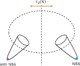
Figure 1: A schematic diagram of the internal space showing the two throats related by the ${\mathbb{Z}}_{2}$ ${\cal R}$ symmetry containing the NS5-brane and the $\overline{\rm NS5}$-brane respectively.

4.5.4 The Subleading Effect Due to pairs

The subleading effect is due to the $\Delta N$ brane-anti brane pairs. The resulting change in the geometry was calculated in [13] for UV of the KS throat, and [14, 15] for IR. As was mentioned it is not simply of the warped form, eq.(4.15). Nevertheless an estimate of the resulting change in volume can be obtained by just keeping the change in the warp factor.

In the region far from the tip of the KS geometry where the pairs are located, the geometry is essentially $AdS_{5}\times{\bf S}^{5}$ and the perturbation goes like,

$$\delta e^{-4A}\sim\Delta Ne^{4A_{0}}R^{4}{g_{s}\alpha^{\prime 2}\over|r|^{8}}$$ (4.36)

where the $e^{4A_{0}}$ factor arises from the warping at the tip of the throat. Note the $1/|r|^{8}$ fall off which is much faster than the $1/|r|^{4}$ fall-off for a D3-brane source . The important point here is that the brane-anti brane pairs give rise to a normalizable deformation in the asymptotic $AdS_{5}\times{\bf S}^{5}$ region, which falls like $1/|r|^{8}$, this deformation is suppressed by $e^{4A_{0}}$ because the warp factor at the bottom of the throat suppresses the energy density of the pair in this manner. While some of the discussion in [13] is in the context of the KS geometry their main result is more general and should apply to other situations as well which are asymptotically $AdS_{5}\times{\bf S}^{5}$, with the warped throat terminating in a region where the warp factor attains a minimum value $e^{A_{0}}$.

The resulting change in $V_{I}$ that eq.(4.36) leads to can be calculated from eq.(4.18). Since our purpose is to make a rough estimate we may as well approximate the geometry to be a region of $AdS_{5}\times{\bf S}^{5}$ with the $AdS_{5}$ being cut-off both in the UV and the IR; i.e., of the type considered in the RS1 model, with metric,

$$ds^{2}={r^{2}\over R^{2}}(dx_{\mu}dx^{\mu})+{R^{2}\over r^{2}}(dr^{2}+r^{2}d\Omega_{5}^{2})$$ (4.37)

where the radial coordinate has range $r_{\rm min}\leq r\leq r_{\rm max}$. This metric has the form, eq.(4.15), with

$$\tilde{g}_{ab}=\delta_{ab}$$ (4.38)

being the flat-space metric. The warp factor at the bottom of the cut-off $AdS$ region is ${r_{\rm min}^{2}/R^{2}}$ which in this crude model should be equated with $e^{2A_{0}}$ at bottom of the KS-like throat giving,

$$r_{\rm min}^{2}=R^{2}e^{2A_{0}}.$$ (4.39)

The brane anti brane pair located at the bottom of the throat produces a change in the warp factor eq.(4.36) and we interested in the change in $V_{I}$ this leads to. Integrating eq.(4.18) using eq.(4.38) gives,

$$\delta V_{I}\sim\Delta Ne^{4A_{0}}R^{4}\alpha^{\prime 2}{g_{s}\over r_{\rm min}^{2}},$$ (4.40)

where we have taken $r_{\rm max}\rightarrow\infty$ since the integral converges in the UV. Next using eq.(4.39) gives,

$$\delta V_{I}\sim\Delta Ne^{2A_{0}}R^{2}\alpha^{\prime 2}.$$ (4.41)

So far we have only estimated the contribution from the region far from the tip of the throat where the pairs of 3-branes are located. We can also try to estimate the contribution from the region near the tip as follows. Let us continue to crudely model the throat as a cut-off $AdS_{5}\times{\bf S}^{5}$ geometry, eq.(4.37) with the pairs located at $r_{\rm min}$. Very close to the sources, it seems reasonable to estimate that the change produced in the warp factor by a D3-$\overline{\mathrm{D}3}$ pair is of order the change produced by a single $\overline{\mathrm{D}3}$-brane. This results in a change in the warp factor,

$$\delta e^{-4A}\sim\delta N{g_{s}\alpha^{\prime 2}\over r^{4}}$$ (4.42)

and a change in $V_{I}$

$$\delta V_{I}\sim\delta N{g_{s}\alpha^{\prime 2}}R^{2}e^{2A_{0}},$$ (4.43)

where in obtaining eq.(4.43) this time, since we are interested in the region close to the brane, we cut off the integral before $r$ gets too large at $r\sim r_{\rm min}$. Note, that this result is parametrically of the same form as the contribution from the region far from the tip eq.(4.41). Adding the effects of the near-and far regions we would therefore expect an answer of the form eq.(4.41).

To complete our analysis we now calculate the resulting term in the axion potential. Since $\Delta N\propto a$ we get from eq.(4.41), eq.(4.23),eq.(4.14) that the extra potential generated for the axion is

$$\delta V\sim U_{\rm mod}e^{2A_{0}}{R^{2}\over\alpha^{\prime}L^{4}}a.$$ (4.44)

The estimate for the near-region can be improved in the context of a KS throat using the results of [14, 15]. This more careful analysis gives results which essentially agree with eq.(4.43), eq.(4.44).

In the above discussion we have not kept track of signs and coefficients. The contribution due to warping eq.(4.41), we will see below, will typically lead to a contribution in the axion potential that dominates over other contributions, including the term due to the induced tension of the D3, $\overline{\mathrm{D}3}$-branes we first considered in eq.(3.21). It will be important for the axion model to work that this net contribution is positive. Our analysis above is too preliminary to allow us to determine this sign. Physically one would expect the net contribution to be positive, since otherwise the added D3-brane charge on the 5-brane anti 5-brane would reduce the energy of the system and this energy would decrease as the charge increased. However, one should clearly try to determine this from a first principles calculation, along with improving the other aspects of this calculation as well. We leave this for future investigation.

4.5.5 Final Conclusions

The changes in $V_{I}$, eq.(4.18), that arise due to warping could possibly manifest themselves in corrections to the superpotential and/or the Kähler potential. For example, ${\rm Re}(T)\sim L^{4}$ in the unwarped case and it is more generally related to the size of the non-trivial four-cycle. Thus $T$ could change once warping effects are included causing in turn changes in the superpotential and the Kähler potential . The warping induced changes might also lead to effects that cannot be incorporated into supersymmetric data in such a ready fashion, since the induced $\overline{\mathrm{D}3}$-brane charge breaks SUSY. Either way the resulting corrections to the axion potential will be given by eq.(4.44), which is the main result from this subsection.

4.6 An Additional Contribution

Before concluding this section let us discuss one additional contribution which will turn out to be unimportant.

There is a correction to the axion potential which arises due to the interaction between the 5-brane and the anti brane in the two different throats. In the limit where the induced D3-brane tension dominates over the 5-brane tension this is simple to estimate. The potential reduces to that calculated between D3 and $\overline{\mathrm{D}3}$-branes calculated in [38]. This gives a result,

$$\delta V\sim{a^{2}\over|r_{1}-r_{2}|^{4}}\epsilon^{2},$$ (4.45)

where the two throats are located at radial coordinates $r_{1},r_{2}$ and for simplicity we have taken the internal space to be flat. Here, $\epsilon=e^{4A_{0}}$, is the warp factor at the bottom of the throat. We see that this contribution is suppressed by an extra factor of $\epsilon$ compared to the tension term calculated in eq.(3.17). Since $\epsilon$ is very small, as the preliminary analysis which actually underestimates $\epsilon$ already found in eq.(3.26), we see that this contribution will be highly suppressed compared to the ones we keep.

5 The Model: A More Complete Look

To summaries, we started with a potential of the form, eq.(3.21),

$$V_{0}=c_{1}{1\over\alpha^{\prime 2}g_{s}}e^{4A_{0}}a.$$ (5.1)

Then we found that corrections will generate an additional term, eq.(4.44). Using the relation eq.(3.12) this can be written in terms of the SUSY breaking scale $M_{SB}$ as,

$$V_{1}=c_{2}M_{SB}^{4}e^{2A_{0}}\left({R^{2}\over\alpha^{\prime}L^{4}}\right)a.$$ (5.2)

Here $L^{6}$ is the volume in string units, and $R$ is roughly speaking the radius of the AdS-like throat regions in which the 5-brane and anti brane’s are placed . In the supergravity approximation

$$R^{2}/\alpha^{\prime}>1.$$ (5.3)

We also note that $e^{A_{0}}$ in eq.(5.1), eq.(5.2), is the warp factor at the bottom of the throat.

The total potential is then linear in the axion and the sum of the two terms,

$$V=V_{1}+V_{1}=\mu^{4}a$$ (5.4)

where the final expression on the RHS can be taken to be the definition of the scale $\mu^{4}$.

We should also note that eq.(5.1) and eq.(5.2) are valid only for $a>0$ and also for sufficiently large values of $a$. The more correct form for $V_{0}$ is in eq.(3.17), we will return to a discussion of corrections to the linear form of the potential in §6.3.

5.1 The Energy Scales

To understand which of the two terms, eq.(5.1) or eq.(5.2) is bigger let us start by first setting $g_{s}=L=1$. This also sets $1/\alpha^{\prime 2}\sim M_{Pl}^{2}$. Also we set ${R^{2}\over\alpha^{\prime}}=1$. Since we have not been able to calculate $c_{2}$ anyways, we also neglect any dependence on the coefficients $c_{1},c_{2}$. Finally we set $a\sim O(1)$ so that $a\sim L^{2}$ as is needed for the slow-roll conditions to be met eq.(3.8). Setting the moduli stabilization contribution $V_{1}$ to be of order the vacuum energy density, we then get,

$$V_{1}\sim M_{SB}^{4}e^{2A_{0}}\sim\Lambda^{4}.$$ (5.5)

This gives $V_{0}$ to be

$$V_{0}\sim{M_{Pl}^{4}\Lambda^{4}\over M_{SB}^{8}}\Lambda^{4}.$$ (5.6)

Now if the SUSY breaking scale is $M_{SB}\sim 1\,{\rm TeV}$,

$${M_{Pl}^{4}\Lambda^{4}\over M_{SB}^{8}}\sim O(1).$$ (5.7)

Thus $V_{0}\sim V_{1}$ and both make roughly an equal contribution to the vacuum energy. However, as the moduli stabilization scale and SUSY breaking scale are raised we see that $V_{0}$ begins to become smaller than $V_{1}$ and less important. For example, when $M_{SB}\sim 10^{10}\,{\rm GeV}$, the intermediate scale, $V_{0}$ is much smaller,

$$(V_{0})^{1/4}\sim 10^{-17}\,{\rm eV}.$$ (5.8)

Let us keep track of the dependence on the volume $L$ and $g_{s}$ also now. We set $a\sim L^{2}/g_{s}$, eq.(2.14). Setting $V_{1}$ to be of order the energy density gives,

$$V_{1}\sim M_{SB}^{4}({R^{2}\alpha^{\prime}})e^{2A_{0}}{a\over L^{4}}\sim M_{SB}^{4}({R^{2}\alpha^{\prime}})e^{2A_{0}}{1\over L^{2}g_{s}}\sim\Lambda^{4}.$$ (5.9)

Solving for $e^{2A_{0}}$ gives,

$$e^{2A_{0}}\sim\left({\Lambda^{4}\over M_{SB}^{4}}\right)g_{s}L^{2}\left({\alpha^{\prime}\over R^{2}}\right).$$ (5.10)

Using the fact that $M_{Pl}^{2}\sim{L^{6}/(\alpha g_{s}^{2})}$ and substituting in eq.(5.1) then gives,

$$V_{0}\sim{g_{s}^{4}\over L^{6}}\left({\alpha^{\prime}\over R^{2}}\right)^{2}\left({M_{Pl}^{4}\Lambda^{4}\over M_{SB}^{8}}\right)\Lambda^{4}.$$ (5.11)

For our approximation of classical supergravity to be valid, $g_{s}<1,L>1,$ and $R^{2}>\alpha^{\prime}$. This means even for $U_{\rm mod}\sim({\rm TeV})^{4}$, $V_{0}<\Lambda^{4}$ and thus $V_{0}$ will be subdominant. Increasing $L,R^{2},$ or decreasing $g_{s}$ will make $V_{0}$ even smaller. Similarly increasing $U_{\rm mod}$ will also reduce $V_{0}$.

Our conclusion is that the second term $V_{1}$, which arises due to the interplay of moduli stabilization and warping caused by the axion getting turned on, is typically the dominant contribution. We must caution the reader that we have not kept track of numerical coefficients, some of these could be large, and our statements here are really only parametric nature.

The warped down string scale at the bottom of the throats where the 5-branes are present is,

$$m_{s}\sim{1\over\sqrt{\alpha^{\prime}}}e^{A_{0}}\sim{M_{Pl}g_{s}\over L^{3}}e^{A_{0}},$$ (5.12)

where in obtaining the last relation we have used eq.(3.3). Supergravity modes (KK modes in the throat region) have a mass which is even lower by a factor of $\sqrt{\alpha^{\prime}}/R_{0}$ where now $R_{0}$ is the radius of curvature at the bottom of the throat .

For the case we discussed first above, around eq.(5.6), with $g_{s}\sim L\sim a\sim R_{0}\sqrt{\alpha^{\prime}}\sim O(1)$ and $M_{SB}=1\,{\rm TeV}$ we see that the warped down string modes and KK modes have a mass of order $10^{-3}\,{\rm eV}$. As $M_{SB}$ rises the mass becomes even lower. For $g_{s}\sim L\sim a\sim R_{0}\sqrt{\alpha^{\prime}}\sim O(1)$ and $M_{SB}\sim 10^{10}\,{\rm GeV}$ this mass is of order $10^{-17}\,{\rm eV}$. Thus there are many very light particles which arise due to string modes and KK modes in the highly warped region. We will have more to say about these light particles in §6.1.

5.2 The Constraints

It is also worth summarizing the constraints on the various parameters of the model.

The slow-roll conditions require that the axion satisfy the condition, eq.(3.8). Our estimate for the $V_{1}$ term in the potential is valid only when the charge contributed by the axion is a small fraction of the total charge supporting each throat, this gives the condition,

$$a\ll N,$$ (5.13)

Using eq.(3.8) and eq.(4.26) this give,

$$L^{2}\ll R^{4}/\alpha^{\prime 2}.$$ (5.14)

Finally the total volume of the internal space is $L^{6}(\alpha^{\prime})^{3}$, this must be bigger than the volume of each warped throat $\sim R^{6}$, leading to

$$L^{4}\gg R^{4}/\alpha^{\prime 2}.$$ (5.15)

The summary is that the conditions,

$$L^{2}<g_{s}a\ll R^{4}/\alpha^{\prime 2}\ll L^{4}$$ (5.16)

must all be met. They are mutually compatible so there is no obstruction to doing so. In addition the scale $\mu^{4}$ defined in eq.(5.4) must meet the condition

$$\mu^{4}a=\Lambda^{4}$$ (5.17)

where $\Lambda$ is defined in eq.(1.1). This does require $\mu$ to be a very small energy, but as was emphasized in §3.2, where a preliminary estimate for $\mu$ was carried out by neglecting $V_{1}$, this can be arranged by choosing a modestly small ratio of fluxes which results in an exponentially small value of $e^{A_{0}}$.

5.3 Additional Comments

Let us end this section with two comments.

First, it could be that despite our best attempts at being careful we have missed some important additional contributions to the axion potential. The following general reasoning suggests that even if this were true, incorporating such effects would probably lead to a workable model within the kind of setup we have explored. One would expect that any additional contribution is linear in $a/N$, as long as $a\ll N$. Also, since the shift symmetry is broken by the 5-branes whose effects are suppressed by $e^{A_{0}}$, such a term should also be suppressed by a positive power of $e^{A_{0}}$. If this power is smaller than $2$, then this additional contribution could dominate over the terms we have kept. However in this case we can simply adjust the warp factor so that the resulting scale $\mu$ in eq.(5.4), after accounting for this term, has the correct value. This will typically make $e^{A_{0}}$ even smaller and thus the particles as the bottom of the warped throats even lighter, but, as we will see in §6.1, this is an acceptable price to pay since these particles do not lead to any observable signals anyways.

Second, in the KKLT construction the negative vacuum energy density that arises after moduli stabilization is canceled by the addition of $\overline{\mathrm{D}3}$-branes which are placed in a warped throat. It is natural to ask whether in our model one can dispense with these $\overline{\mathrm{D}3}$-branes and their attendant throat, and instead cancel the negative vacuum energy by the axion dependent contributions, eq.(5.4).

A simple calculation shows though that this would require too many units of flux $N$ stabilizing the 5-brane throats. Let the negative energy generated by moduli stabilization be $-C$, including it in the total potential gives,

$$V=\mu^{4}a-C.$$ (5.18)

The constant $C$ can be absorbed by shifting the axion

$$a\rightarrow a+\Delta a$$ (5.19)

with

$$\Delta a=C/\mu^{4}.$$ (5.20)

The resulting analysis in terms of the shifted axion then exactly agrees with what we had done earlier, when $C=0$. Since the shifted axion must satisfy the condition, eq.(3.8), (to get a model of quintessence) equating $V$ with $\Lambda^{4}$ now will again lead to the conclusion that

$$\mu^{4}<\Lambda^{4},$$ (5.21)

for $L>1,g_{s}<1$. The resulting shift is therefore

$$\Delta a={U_{\rm mod}\over\mu^{4}}>{({\rm TeV})^{4}\over\Lambda^{4}}=10^{60},$$ (5.22)

where we have used the fact that $C=U_{\rm mod}\geq O({\rm TeV})^{4}$. The linear potential we have used though is valid only when eq.(5.13) is true and this condition involves the total value of the axion including its shift. Thus the large value of $\Delta a$ would require a large amount of flux $N$, which makes this idea implausible.

Our model therefore must incorporate the two throats with the 5-branes and at least one additional throat (or perhaps two which are related by the ${\mathbb{Z}}_{2}$ symmetry) to contain the $\overline{\mathrm{D}3}$-branes of the KKLT setup.

6 Some Features of The Model

We now turn to discussing some general features of the model.

6.1 Many Light Particles:

The model has many light particles. We saw that the warped down string scale at the bottom of the two throats where the 5-branes are located is at least $10^{-3}\,{\rm eV}$ and typically is much lighter for a scale of SUSY breaking $M_{SB}>1\,{\rm TeV}$ . Thus there are many very light particles in the theory which come from string modes and Kaluza Klein modes localized in the warped region.

One might be worried that so many light particles would be in conflict with observation. However, this is not so. The model is in fact closely related to the Randall-Sundrum II model (RS II) [40] in which there is only one brane called the Planck brane. More accurately it is akin to a Randall Sundrum I model (RS I) [41] but with the warped down energy scale at the “Standard Model” brane being $10^{-3}\,{\rm eV}$ or much lower. The RS II model can be thought of as a limit of RS I where the standard model brane is moved away to infinity resulting in a non-compact dimension.

We take the standard model degrees of freedom to not live in the two throat regions where the 5-branes are located. In terms of the RS model they are then degrees of freedom on the Planck brane. The four-dim. graviton is a non-normalizable mode in $AdS_{5}$ and is localized on the Planck brane as well. The first thing to note is that the throat regions make a finite contribution, of order $R^{6}$, to the volume of the internal space where $R$ is given in eq.(4.26) and $N$ are the number of five-form flux units supporting the throat. As a result the $4$ dim. Newton’s constant is finite and as we have discussed above can take the required value consistent with the other constraints of the model. In addition the couplings of the matter fields with the KK modes in the throat are suppressed so that corrections to Newton’s gravitational law due to KK exchange and corrections to energy loss in gravitational radiation are suppressed by a factor of $(pR)^{2}$ compared to the leading answers which neglect these KK modes, where $p$ is the characteristic energy scale involved. Now in the model the flux units $N$ and thus $R$ has to be big enough to meet the condition eq.(5.16), however this can be typically arranged by taking $R$ to be not very different from the Planck scale. As a result this suppression is very significant and results in no detectable signal. E.g., taking $N\sim 1000$, $g_{s}\sim O(1)$, eq.(5.16) can be met for $L\sim O(10)$, and $a\sim O(100)$. In this case, $R^{-1}\sim 10^{16}\,{\rm GeV}$ so that the suppression is of order $(p/10^{16}\,{\rm GeV})^{2}$ and is indeed very significant. Finally as argued in [40] the interactions between the four-dim. graviton and KK modes are also highly suppressed, because the four-dim. graviton is localized on the Planck brane and a typical KK mode is localized deep inside the $AdS$ region.

Besides light particles in the two throats, there are also moduli, not localized in the throats, which are stabilized by $U_{\rm mod}$ (e.g., the overall volume). These have a mass

$$m_{\rm moduli}^{2}\sim{U_{\rm mod}\over M_{Pl}^{2}}.$$ (6.1)

For $U_{\rm mod}\sim{\rm TeV}^{4}$ this is also a mass of order $10^{-3}$   eV. As the scale of moduli stabilization is increased the masses of these moduli increase, while, as we have seen above, typically the masses of the warped down string states and the KK states move down.

In constructing a complete cosmological model one would have to deal with the moduli problem [42, 43] that arises due to all these light modes. Perhaps after high-scale inflation one can arrange so that the KK and string modes in the warped throats are not significantly excited and the moduli like the overall volume which are spread out over the whole CY are either heavy enough to not cause a problem, or are rendered unproblematic by symmetry considerations, [44], or by thermal inflation [45].

In particular it is important to ensure that the two throats are not excited to even small finite temperature. This would cause a black brane metric to replace the throat geometry at the tip, the two NS5-branes would then fall into the horizon of the black brane and the resulting equation of state would be more akin to a thermal gas and unsuitable for quintessence. This is especially a concern because of the low warped down energy scale at the bottom of the throat.

If reheating after inflation results in entropy being dumped into standard model fields, this can probably be ensured. The suppressed interactions with the throat excitations will then prevent the throat degrees of freedom from coming into equilibrium with the standard model degrees as long as the temperature after reheating is somewhat lower than the GUT scale, and this can prevent the formation of a black brane horizon .

6.2 Rotation of The CMB Polarization

It is well known that an axion $a$, which is a pseudoscalar, can couple to the photon through the

$$\Delta L=\zeta aF\tilde{F}$$ (6.2)

term in the Lagrangian causing the E mode of the CMB to be rotated into the B mode [46, 47, 20]. Here $\zeta$ is a constant coefficient. Such a coupling also causes the direction of linearly polarized light to rotate in the course of propagation from a distant source [48].

The extent of rotation of the E mode to the B mode is parameterized by an angle

$$\Delta\alpha\sim\zeta\Delta a$$ (6.3)

where $\Delta a$ is the total change in the axion due to its time evolution.

CMB experiments put a bound on $\Delta\alpha$. The bound in [25] is

$$\Delta\alpha=-1.1\deg\pm 1.3\deg({\rm stat.})\pm 1.5\deg({\rm syst.})\ \ \ (68\%\ {\rm CL})$$ (6.4)

which is currently consistent with $\Delta\alpha$ vanishing.

A significant limitation of this paper is that we have not discusses how the standard model arises in our construction. As a result we do not know whether a coupling of the type in eq.(6.2) in fact arises. In fact it is more or less clear that such a coupling cannot arise in a SUSY preserving manner. For that to happen the SUSY partner of the axion would have to play the role of the QED coupling constant. Typically this happens only if the axion partner is a non-compact scalar. In our model where the axion arises from $C_{2}$, however, its partner arises from $B_{2}$ and therefore is a compact scalar.

The coupling to electromagnetism could arise though in a SUSY non-invariant way and this could well be allowed if SUSY is broken at a sufficiently high scale. In particular, such a coupling would arise if the $U(1)$ gauge group of the SM arose from a D5-brane wrapping the same two cycle which gives rise to the zero mode for the axion. On the world-volume of the D5-brane would be the couplings,

$$S=(2\pi\alpha^{\prime 2})T_{5}\left[\int d^{6}x\sqrt{-g}{1\over 4}F_{\mu\nu}F^{\mu\nu}+{1\over 2}\int C_{2}\wedge F\wedge F\right].$$ (6.5)

Reducing to $4$ dimensions gives,

$$S=(2\pi\alpha^{\prime 3})T_{5}\left[L^{2}\int d^{6}x\sqrt{-g}{1\over 4}F_{\mu\nu}F^{\mu\nu}+{1\over 2}a\int F\wedge F\right].$$ (6.6)

Now redefining $F_{\mu\nu}$ so that the gauge kinetic term is canonical we see that the coupling $\zeta$ in eq.(6.2) is

$$\zeta={1\over L^{2}}.$$ (6.7)

As a result

$$\Delta\alpha\sim{1\over L^{2}}\delta a.$$ (6.8)

Using the observed limits in eq.(6.4) (converted to radians) we then get

$${\Delta a\over L^{2}}<10^{-2}.$$ (6.9)

The canonically normalized field is $\phi=f_{a}a\sim{a\,g_{s}M_{Pl}}/L^{2}$ as in eq.(3.7). The change in $\phi$ is given in eq.(2.24), using eq.(6.9) this gives,

$${M_{Pl}\over\phi}\lesssim 10^{-2}g_{s}\lesssim 10^{-2},$$ (6.10)

where we have used the fact that $g_{s}<1$. This tells us that to be in agreement with the bound eq.(6.4) the canonically normalized field must have a value which is at least two orders of magnitude bigger than the Planck scale. As a result the axion field will evolve very little in the course of the universe’s evolution. The slow roll parameter $\epsilon$, eq.(2.19), for example would satisfy the condition

$$\epsilon\lesssim 10^{-4}.$$ (6.11)

This makes the equation of state for quintessence essentially indistinguishable from the cosmological constant.

In summary, we do not know for certain whether the axion couples to electromagnetism in the form of eq.(6.2). Such a coupling would arise if the $U(1)$ gauge field originates on a D5-brane wrapping the same two-cycle from which the axion zero mode also arises. In this case the bound on the rotation put by CMB data is very significant. It requires the canonically normalized axion field to change very little during the course of the evolution of the universe, thereby making the equation of state for quintessence essentially like the cosmological constant. In such a situation our best hope for telling quintessence apart from the cosmological constant would be to look for a signal in the rotation for the CMB polarization itself.

6.3 The Linear Potential

The linear nature of the axion potential is valid for an appropriate range of axion values, we took this form in our discussions above to simplify the analysis.

The $V_{0}$ contribution in eq.(5.1) comes from the induced 3-brane tension and its more accurate form is in eq.(3.17) with $\epsilon=e^{4A_{0}}$, as noted in §3.2. As the axion runs towards its minimum at $a\rightarrow 0$ the correction due to the $L^{4}$ term within the square root in eq.(3.17) will become more important.

Also, if we allow for both negative and positive values of the axion, $a$ in eq.(5.1), eq.(5.2) should be replaced by $|a|$. E.g, the more correct form for $V_{1}$ is

$$V_{1}=c_{2}M_{SB}^{4}e^{2A_{0}}\left({R^{2}\over\alpha^{\prime}L^{6}}\right)|a|,$$ (6.12)

which arises because the change in the volume induced by the warping only depends on $|a|$.

With $c_{2}>0$ (which makes physical sense) the total potential $V_{0}+V_{1}$ is positive. Now actually there is an overall constant $C$ in the potential, related to the cosmological constant, which we have not worried about. Including this we get the potential to be,

$$V_{\rm total}=V_{0}+V_{1}+C.$$ (6.13)

It is worth emphasizing here that the $V_{1}$ contribution is linear in the axion only in the limit when $|a|\ll N$ where $N$ is the total five -form flux supporting the warped throats where the $5$ branes are placed. Once $|a|$ becomes larger there will be corrections and one does not expect the potential to remain linear in the axion, for example the warp factor $e^{A_{0}}$ at the bottom of the throat will itself begin to depend on $a$. As was noted in §4.3 with todays’ knowledge of warped compactifications we have at best been able to estimate the linear corrections, calculating the higher order terms is even harder. For now, we note the possibility that including these terms might well give a more rapidly varying axion potential for $|a|>N$, and the more rapidly varying potential might actually help improve the tracker behavior of this model, to which we turn next.

6.4 Tracker Behavior

It is well known that many quintessence models exhibit tracker behavior, see e.g., [3]. The tracker solution is an attractor, and at least for some range of initial conditions the system is drawn to the tracker solution regardless of initial conditions.

Here let us consider the linear potential case, with the net potential being given by eq.(5.4). The equation of motion for the axion is given by

$$\ddot{\phi}+3H\dot{\phi}+{\mu^{4}\over f_{a}}=0$$ (6.14)

Let us assume that the universe is radiation dominated, then

$$H={1\over 2t}.$$ (6.15)

The general solution to eq.(6.14) is

$$\phi=c_{1}-{\mu^{4}\over 5f_{a}}t^{2}+c_{2}t^{-{1\over 2}}$$ (6.16)

where $c_{1},c_{2}$ are integration constants. We see that the axion runs to the origin, where its energy is minimized in a time determined by $c_{1}$.

Let us take the solution with $c_{2}=0$ and some fixed value of $c_{1}$ and examine perturbations around it. There are two kinds of such perturbations. One is time independent and simply shifts $c_{1}$, the second dies like $t^{-{1\over 2}}$. Since the first perturbation is constant in time we see that this solution is not really a tracker.

Working instead in an epoch which is matter dominated sets $H=2/3t$, the essential features of the axion solution found above continue to be the same in this case as well.

6.5 The Cosmological Constant

The lack of tracker behavior means that our model does not solve the coincidence problem. The initial value for the axion, $c_{1}$, must be chosen to be just right so energy in the axion field is of the right order of magnitude today when the Hubble constant has value $H_{0}$.

In fact this feature is tied to the issue of the cosmological constant in this model which we have mostly ignored so far. Including the constant $C$ in the total potential, eq.(6.13), and working with the linear potential as an approximation we have,

$$V_{\rm total}=\mu^{4}|a|+C$$ (6.17)

where we now keep track of the fact that the potential really depends on $|a|$.

It is now clear that changing the initial conditions for the axion in effect changes $C$. Another way to say this is that shifting $a$ and then changing $C$ appropriately can keep $V_{\rm total}$ and in fact the full axion Lagrangian eq.(2.12) invariant .

An important idea, for which the landscape of string theory has now provided considerable evidence, is that the cosmological constant takes its small value due to anthropic considerations, see, e.g., [49, 50, 51]. Let us consider how such anthropic considerations might work in our model . Let us take the constant $C$ and the initial condition for the axion $c_{1}$ as the two variable which can be varied. One possibility is that the axion sits at its minimum at $a=0$ and dark energy is entirely due to the cosmological constant with $C$ taking the value $\Lambda^{4}$ due to anthropic considerations. But the more general possibility is that the total energy in dark energy is shared more equitably between the cosmological constant and the axion field with both $C$ and $\mu^{4}|a|$ being of order $\Lambda^{4}$. In this latter case, the equation of state for dark energy could show significant time variation. In fact, knowing nothing better, one would tend to believe that this latter possibility is more likely, simply because it is more general. Of course deciding this issue more systematically would require a well motivated probability measure in the space of all possibilities, which we lack at the moment.

Let us emphasize that it was important in the discussion of this subsection that the axion potential is slowly varying. Instead suppose the scale in the potential eq.(5.4) is, $\mu^{4}\sim M_{SB}^{4}$, which is the SUSY breaking scale. Then starting with $c_{1}\sim M_{Pl}$ and taking $f_{a}\sim M_{Pl}$ for simplicity, we find that the axion field runs to its minimum in time $t\sim{M_{Pl}/M_{SB}^{2}}$ which is of order the Hubble constant at the time of SUSY breaking. This is too fast to be of any relevance today.

7 Conclusions

In this paper we have constructed a model for quintessence in string theory. The model is based on the idea of axion monodromy. An axion plays the role of the quintessence field, its shift symmetry is broken by the presence of $5$-branes which are located in highly warped throats. We show that even after including the effects of moduli stabilization and SUSY breaking, the resulting potential for the axion can be made slowly enough varying to result in a workable model of quintessence. If the canonically normalized axion field has an initial expectation value of order the Planck scale, the equation of state of dark energy shows significant time variation during the evolution of the universe.

Our model has many light particles which arise due to the highly warped throats in which the 5-branes are placed. The energy scale at the bottom of these throats is at least $10^{-3}\,{\rm eV}$ and typically is much lower. The light particles arise from warped down string modes or KK modes and are analogous to the light particles in the Randall Sundrum II model which has only the Planck brane with a non-compact extra direction. The couplings of these particles to standard model fields and to the four dimensional graviton are highly suppressed, making them difficult to detect.

We have not attempt to construct a complete model of cosmology, including for example inflation at early times. We have also not attempted to explicitly incorporate the standard model fields in the kind of construction we used. This latter issue especially deserves further attention because a coupling of the axion to electromagnetism would lead to a rotation of the E mode of polarization of the CMB to the B mode, with potential observable consequences. We show how such a coupling can arise in our model when the photon is the gauge field living on a D5-brane and calculate the resulting rotation effect.

The cosmological constant question is still left open in our discussion. Anthropic considerations could well be responsible for its smallness. We suggest that these considerations, in the context of our model, would probably lead to the conclusion that the axion field is not exactly at its minimum. Rather, it is more likely to be rolling and carrying a reasonable fraction of the total dark energy, thereby causing the equation of state for dark energy to vary. Models of the type we present here, where the potential for the quintessence field is slowly enough varying, might therefore tilt the “betting odds” in favor of quintessence, even though they lack an explanation for the cosmological constant along conventional, as opposed to anthropic, lines.

References

- [1] L. McAllister, E. Silverstein, and A. Westphal, “Gravity Waves and Linear Inflation from Axion Monodromy,” Phys. Rev. D82 (2010) 046003, arXiv:0808.0706 [hep-th].
- [2] S. Weinberg, Cosmology. 2008. Oxford, UK: Oxford Univ. Pr. (2008) 593 p.
- [3] P. J. E. Peebles and B. Ratra, “The cosmological constant and dark energy,” Rev. Mod. Phys. 75 (2003) 559–606, arXiv:astro-ph/0207347.
- [4] E. V. Linder, “The Dynamics of Quintessence, The Quintessence of Dynamics,”Gen. Rel. Grav. 40 (Apr., 2008) 329–356, 0704.2064.
- [5] E. J. Copeland, M. Sami, and S. Tsujikawa, “Dynamics of dark energy,” Int. J. Mod. Phys. D15 (2006) 1753–1936, hep-th/0603057.
- [6] S. Tsujikawa, “Dark energy: investigation and modeling,” 1004.1493.
- [7] E. Witten, “The cosmological constant from the viewpoint of string theory,” hep-ph/0002297.
- [8] P. Svrcek, “Cosmological constant and axions in string theory,” arXiv:hep-th/0607086.
- [9] P. Svrcek and E. Witten, “Axions in string theory,” JHEP 06 (2006) 051, arXiv:hep-th/0605206.
- [10] E. Silverstein and A. Westphal, “Monodromy in the CMB: Gravity Waves and String Inflation,” Phys. Rev. D78 (2008) 106003, arXiv:0803.3085 [hep-th].
- [11] R. Flauger, L. McAllister, E. Pajer, A. Westphal, and G. Xu, “Oscillations in the CMB from Axion Monodromy Inflation,”JCAP 1006 (July, 2010) 009, 0907.2916.
- [12] S. Kachru, R. Kallosh, A. D. Linde, and S. P. Trivedi, “De Sitter vacua in string theory,” Phys. Rev. D68 (2003) 046005, arXiv:hep-th/0301240.
- [13] O. DeWolfe, S. Kachru, and M. Mulligan, “A Gravity Dual of Metastable Dynamical Supersymmetry Breaking,” Phys. Rev. D77 (2008) 065011, arXiv:0801.1520 [hep-th].
- [14] P. McGuirk, G. Shiu, and Y. Sumitomo, “Non-supersymmetric infrared perturbations to the warped deformed conifold,” Nucl. Phys. B842 (2010) 383–413, arXiv:0910.4581 [hep-th].
- [15] I. Bena, M. Grana, and N. Halmagyi, “On the Existence of Meta-stable Vacua in Klebanov- Strassler,” JHEP 09 (2010) 087, arXiv:0912.3519 [hep-th].
- [16] A. D. Linde, “Inflation and quantum cosmology,” in ”Three hundred years of gravitation”. Cambridge Univ. Press, Eds. Hawking, S.W. and Israel, W (1987) 604–630.
- [17] J. Garriga and A. Vilenkin, “On likely values of the cosmological constant,” Phys. Rev. D61 (2000) 083502, astro-ph/9908115.
- [18] J. Garriga, A. D. Linde, and A. Vilenkin, “Dark energy equation of state and anthropic selection,” Phys. Rev. D69 (2004) 063521, hep-th/0310034.
- [19] N. Kaloper and L. Sorbo, “Where in the String Landscape is Quintessence,” Phys. Rev. D79 (2009) 043528, arXiv:0810.5346 [hep-th].
- [20] A. Arvanitaki, S. Dimopoulos, S. Dubovsky, N. Kaloper, and J. March-Russell, “String Axiverse,”Phys. Rev. D81 (May, 2010) 123530, 0905.4720.
- [21] A. Arvanitaki and S. Dubovsky, “Exploring the String Axiverse with Precision Black Hole Physics,” 1004.3558.
- [22] X. Dong, B. Horn, E. Silverstein, and A. Westphal, “Simple exercises to flatten your potential,” 1011.4521.
- [23] T. Banks, M. Dine, P. J. Fox, and E. Gorbatov, “On the possibility of large axion decay constants,” JCAP 0306 (2003) 001, hep-th/0303252.
- [24] N. Arkani-Hamed, L. Motl, A. Nicolis, and C. Vafa, “The string landscape, black holes and gravity as the weakest force,” JHEP 06 (2007) 060, hep-th/0601001.
- [25] E. Komatsu et al., “Seven-Year Wilkinson Microwave Anisotropy Probe (WMAP) Observations: Cosmological Interpretation,” 1001.4538.
- [26] S. B. Giddings, S. Kachru, and J. Polchinski, “Hierarchies from fluxes in string compactifications,” Phys. Rev. D66 (2002) 106006, arXiv:hep-th/0105097.
- [27] M. R. Douglas and S. Kachru, “Flux compactification,” Rev. Mod. Phys. 79 (2007) 733–796, arXiv:hep-th/0610102.
- [28] T. W. Grimm and J. Louis, “The effective action of N = 1 Calabi-Yau orientifolds,” Nucl. Phys. B699 (2004) 387–426, hep-th/0403067.
- [29] S. Gukov, C. Vafa, and E. Witten, “CFT’s from Calabi-Yau four-folds,” Nucl. Phys. B584 (2000) 69–108, arXiv:hep-th/9906070.
- [30] I. R. Klebanov and M. J. Strassler, “Supergravity and a confining gauge theory: Duality cascades and chiSB-resolution of naked singularities,” JHEP 08 (2000) 052, arXiv:hep-th/0007191.
- [31] V. Balasubramanian, P. Berglund, J. P. Conlon, and F. Quevedo, “Systematics of Moduli Stabilisation in Calabi-Yau Flux Compactifications,” JHEP 03 (2005) 007, hep-th/0502058.
- [32] A. R. Frey, G. Torroba, B. Underwood, and M. R. Douglas, “The Universal Kaehler Modulus in Warped Compactifications,” JHEP 01 (2009) 036, arXiv:0810.5768 [hep-th].
- [33] S. B. Giddings and A. Maharana, “Dynamics of warped compactifications and the shape of the warped landscape,” Phys. Rev. D73 (2006) 126003, arXiv:hep-th/0507158.
- [34] G. Shiu, G. Torroba, B. Underwood, and M. R. Douglas, “Dynamics of Warped Flux Compactifications,” JHEP 06 (2008) 024, arXiv:0803.3068 [hep-th].
- [35] M. R. Douglas and G. Torroba, “Kinetic terms in warped compactifications,” JHEP 05 (2009) 013, arXiv:0805.3700 [hep-th].
- [36] J. M. Maldacena and H. S. Nastase, “The supergravity dual of a theory with dynamical supersymmetry breaking,” JHEP 09 (2001) 024, hep-th/0105049.
- [37] S. Kachru, J. Pearson, and H. L. Verlinde, “Brane/Flux Annihilation and the String Dual of a Non- Supersymmetric Field Theory,” JHEP 06 (2002) 021, arXiv:hep-th/0112197.
- [38] S. Kachru et al., “Towards inflation in string theory,” JCAP 0310 (2003) 013, hep-th/0308055.
- [39] I. Bena, G. Giecold, M. Grana, and N. Halmagyi, “On The Inflaton Potential From Antibranes in Warped Throats,” arXiv:1011.2626 [hep-th].
- [40] L. Randall and R. Sundrum, “An alternative to compactification,” Phys. Rev. Lett. 83 (1999) 4690–4693, hep-th/9906064.
- [41] L. Randall and R. Sundrum, “A large mass hierarchy from a small extra dimension,” Phys. Rev. Lett. 83 (1999) 3370–3373, arXiv:hep-ph/9905221.
- [42] T. Banks, D. B. Kaplan, and A. E. Nelson, “Cosmological Implications of Dynamical Supersymmetry Breaking,” Phys. Rev. D49 (1994) 779–787, hep-ph/9308292.
- [43] B. de Carlos, J. A. Casas, F. Quevedo, and E. Roulet, “Model independent properties and cosmological implications of the dilaton and moduli sectors of 4-d strings,” Phys. Lett. B318 (1993) 447–456, hep-ph/9308325.
- [44] M. Dine, L. Randall, and S. D. Thomas, “Supersymmetry breaking in the early universe,” Phys. Rev. Lett. 75 (1995) 398–401, hep-ph/9503303.
- [45] D. H. Lyth and E. D. Stewart, “Thermal inflation and the moduli problem,” Phys. Rev. D53 (1996) 1784–1798, hep-ph/9510204.
- [46] S. M. Carroll, G. B. Field, and R. Jackiw, “Limits on a Lorentz and Parity Violating Modification of Electrodynamics,” Phys. Rev. D41 (1990) 1231.
- [47] A. Lue, L.-M. Wang, and M. Kamionkowski, “Cosmological signature of new parity-violating interactions,” Phys. Rev. Lett. 83 (1999) 1506–1509, astro-ph/9812088.
- [48] D. Harari and P. Sikivie, “Effects of a Nambu-Goldstone boson on the polarization of radio galaxies and the cosmic microwave background,” Phys. Lett. B289 (1992) 67–72.
- [49] S. Weinberg, “Anthropic Bound on the Cosmological Constant,” Phys. Rev. Lett. 59 (1987) 2607.
- [50] J. D. Barrow, F. J. Tipler, and J. A. Wheeler, The Anthropic Cosmological Principle. Oxford University Press, 1986.
- [51] C. J. Hogan, “Why the universe is just so,” Rev. Mod. Phys. 72 (2000) 1149–1161, astro-ph/9909295.