Visualization of Data from Integral Field
Spectroscopy and the P3d Tool

Abstract

Integral Field Spectroscopy is a powerful observing technique for Astronomy that is becoming available at most ground-based observatories as well as in space. The complex data obtained with this technique require new approaches for visualization. Typical requirements and the p3d tool, as an example, are discussed.

1 Integral Field Spectroscopy

Integral Field Spectroscopy (IFS), which is – somewhat confusingly – also called “3D” or “tri-dimensional” spectroscopy”, “two-dimensional” or “area” spectroscopy and so forth, and which is known in other areas beyond astronomy under terms like e.g. “hyperspectral imaging”, is a powerful observing technique that has been introduced and refined over the past two decades. It is now at the verge of becoming a standard tool, which is available at most modern telescopes Roth (2010). For practical reasons, some users have, furthermore, adopted the intuitively descriptive terminology “3D” as a reference to the datacube, which is thought to be the product of an observation (cf. Fig. 1).

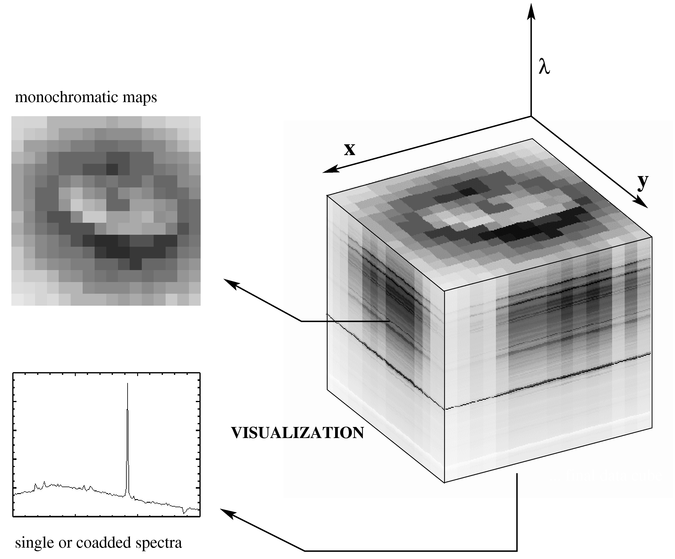
Figure 1: Three-dimensional dataset as the result from IFS (there are two spatial coordinates and one wavelength coordinate). The datacube can be visualized as a stack of quasi-monochromatic images, or, alternatively, as an assembly of $n\times m$ spectra.

IFS is an astronomical observing method that in a single exposure creates spectra of (typically many) spatial elements (“spaxels”) simultaneously over a two-dimensional field-of-view (FoV) on the sky. Owing to this sampling method, each spaxel can be associated with its individual spectrum. Once all of the spectra have been extracted from the detector frame, in the data-reduction process, it is possible to reconstruct maps at arbitrary wavelengths. For instruments with an orthonormal spatial sampling geometry, the spectra can be arranged on the computer to form a three-dimensional array, which is most commonly called a “datacube”. Datacubes are also well-known as the natural data product in radio astronomy. However, there are many integral field spectrographs which do not sample the sky in an orthonormal system. In this case the term datacube is misleading. Also, atmospheric effects, in particular in the optical wavelength regime, make the term inappropriate in the most general case.

Instruments that create three-dimensional datasets in the above mentioned sense, however not simultaneously but rather in some process of sequential data acquisition (scanning) – e.g. tunable filter (Fabry-Perot) instruments, scanning long-slits, etc. – are not strictly 3D spectrographs according to this definition.

Image Dissection, Spatial Sampling, Spectra

Integral field spectrographs have been built based on different methods of dissecting the FoV into spaxels, e.g. optical fiber bundles, lens arrays, optical fibers coupled to lens arrays, or slicers (Fig. 2).

The term spaxel was introduced in order to distinguish spatial elements in the image plane of the telescope from pixels, which are the spatial elements in the image plane of the detector (Kissler-Patig et al. 2004). The optical elements that accomplish the sampling of the sky are often called “integral field units” (IFUs), and IFS is also sometimes called “IFU spectroscopy”. Spaxels can have different shapes and sizes, depending on instrumental details and the type of IFU (Fig. 3).

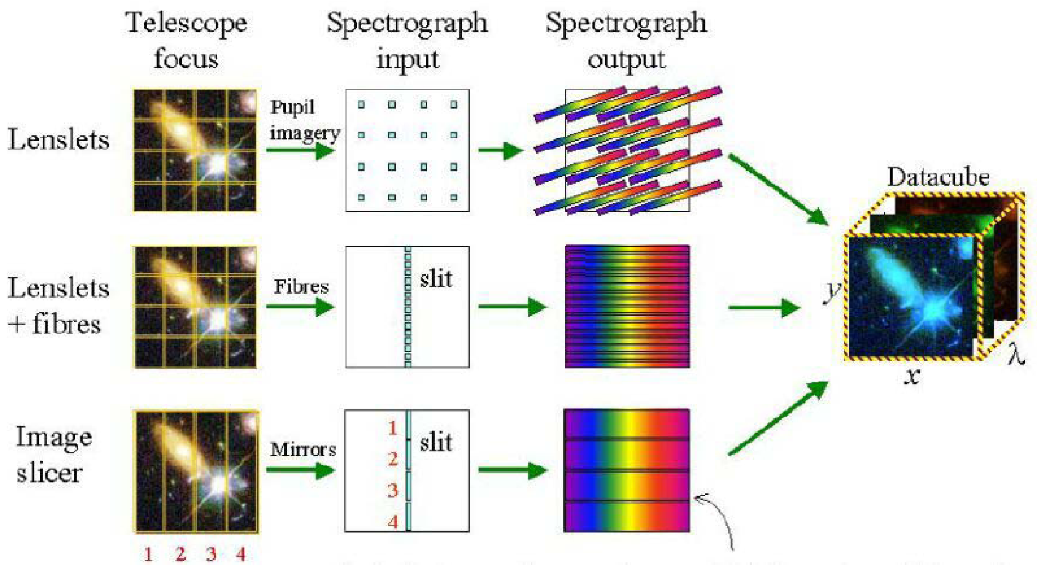
Figure 2: The three major principles of operation of present-day IFUs (source: J.Allington-Smith).

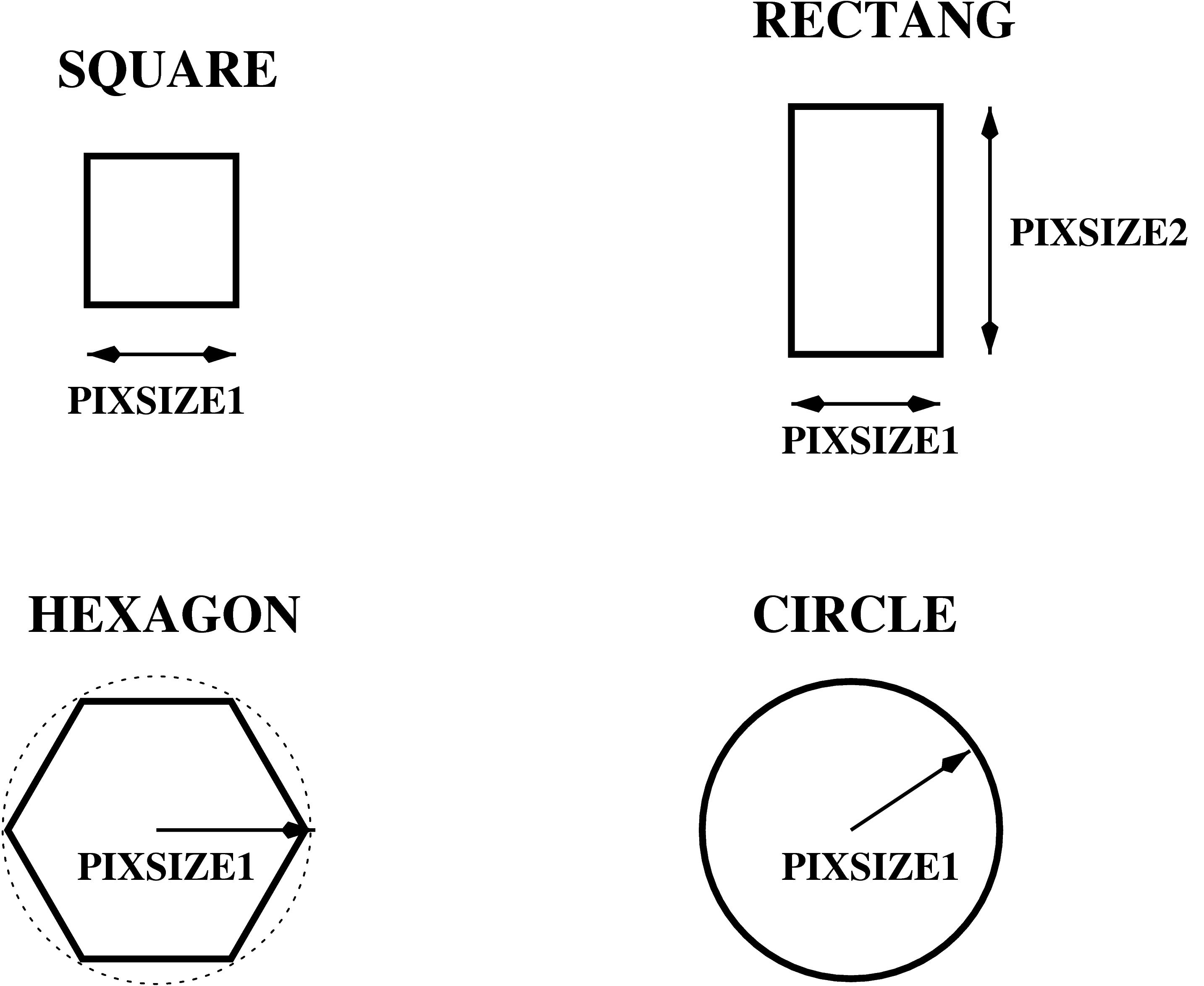
Figure 3: Four different types of spaxel geometries: square, rectangular, hexagonal, and bare fiber (circular).

Contrary to the persuasive implication of the datacube picture, IFUs do not necessarily sample the sky on a regular grid: e.g. fiber bundles, where, due to the manufacturing process, individual fibers cannot be arranged to arbitrary precision. Even if the manufacture of an IFU allows to create a perfectly regular sampling pattern, e.g. in the case of a hexagonal lens array, the sampling is not necessarily orthonormal. Moreover, real optical systems create aberrations and, sometimes, non-negligible field distortions, in which case the spectra extracted from the detector do not sample an orthogonal FoV on the sky. Furthermore, the sampling method may be contiguous (e.g. lens array) fith a fill factor very close to unity, or non-contiguous (e.g. fiber bundle) with a fill factor of significantly less than 100%. In all of these cases, it is possible to reconstruct maps at a given wavelength through some process of interpolation and, repeating this procedure over all wavelengths, to convert the result into a datacube. Note, however, that interpolation often produces artifacts and generally involves loss of information.

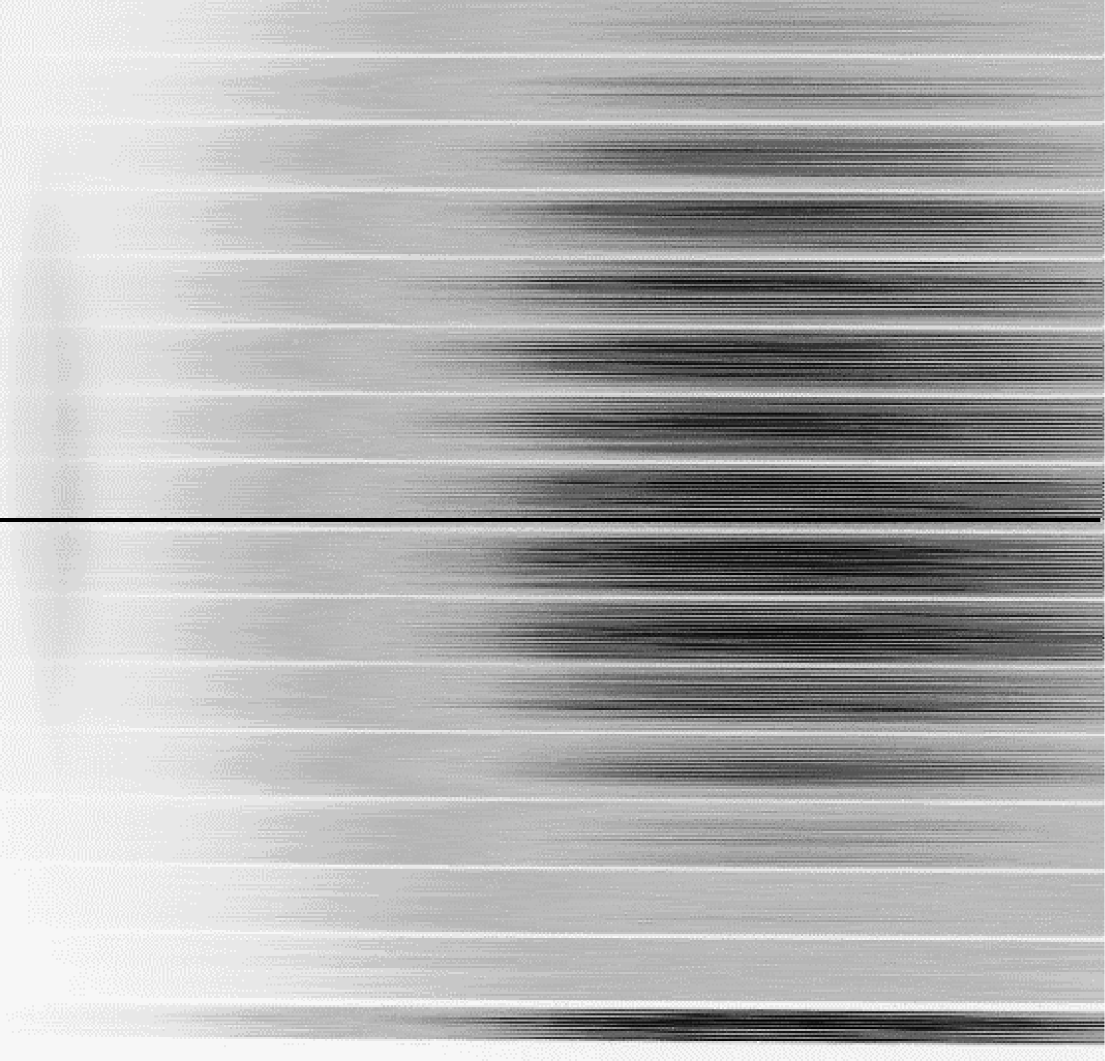
Figure 4: Extraction of IFU spectra from a raw CCD frame.

Data Formats

The generic data product from IFS is a set of spectra, which are associated with a corresponding set of spaxel positions. The spaxel coordinate system may or may not be ortho-normal, but in the most general case it is not. It is only through the process of interpolation in the spatial coordinate system that arbitrary IFU geometries are converted to ortho-normal, i.e. a datacube compatible form. Interpolation, however, inevitably incurs loss of information. Therefore the Euro3D consortium has introduced a special data format for transportation of reduced 3D data which is different from the seemingly simple application of the standard FITS NAXIS=3 format, which is suitable e.g. for radio astronomy (Wells et al. 1981). The Euro3D data format (Kissler-Patig et al. 2004) avoids this latter step of interpolation and assumes only that the basic steps of data reduction have been applied to remove the instrumental signature, but else presenting the data as a set of spectra with corresponding positions on the sky. This approach leaves spatial interpolation and the creation of maps the process of data visualization and analysis, i.e. under control of the user. Figure 5 illustrates the spaxel-oriented approach of the Euro3D FITS data format.

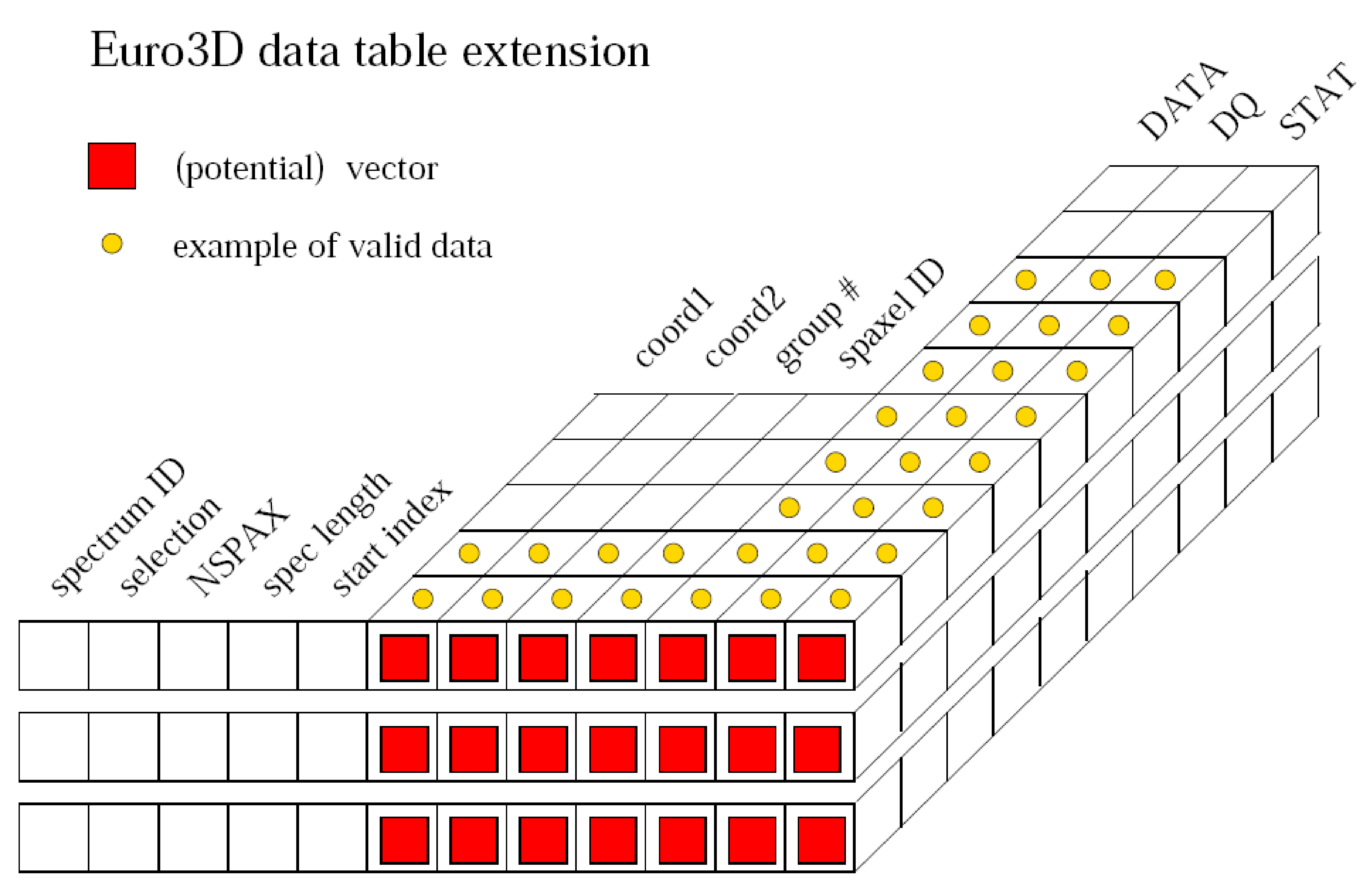
Figure 5: The Euro3D data format (from Kissler-Patig et al. 2004).

2 IFS Visualization

The visualization of IFS data is confronted with two fundamental requirements: the inspection of data for the purpose of monitoring data quality and correcting defects, and the analysis of data, i.e. the derivation of physically meaningful quantities. Ideally, a visualization tool should support both. While the former issue requires to preferentially look into basic elements of a dataset – for example to identify detector faults that mimic a signal, to check the correctness of the various calibration steps (bias subtraction, flat-field and wavelength calibration, extraction of spectra) and so forth – the latter addresses several possible projections of the data set. For example, the user is often interested in obtaining a map at one or several wavelengths over the FoV, corresponding, for example, to emission lines of an extended gaseous object – in order to create line ratio maps, from which one can derive quantities like electron temperature, density, dust extinction etc. On the other hand, for a subset of spaxels that cover a peculiar object, one might wish to co-add the flux within a user-defined aperture, and plot the resulting spectrum.

The p3d software (Sandin et al. 2010) is a versatile data reduction package for optical fiber based 3D instruments, which contains a visualization tool that supports a variety of these needs. Its capabilities are illustrated in Figs. 6–9.

p3d is a free distribution that is licensed under GPLv3. It is available from the project website at http://p3d.sourceforge.net. Although p3d is coded using the Interactive Data Language (IDL) it can be used with full functionality without an IDL license.

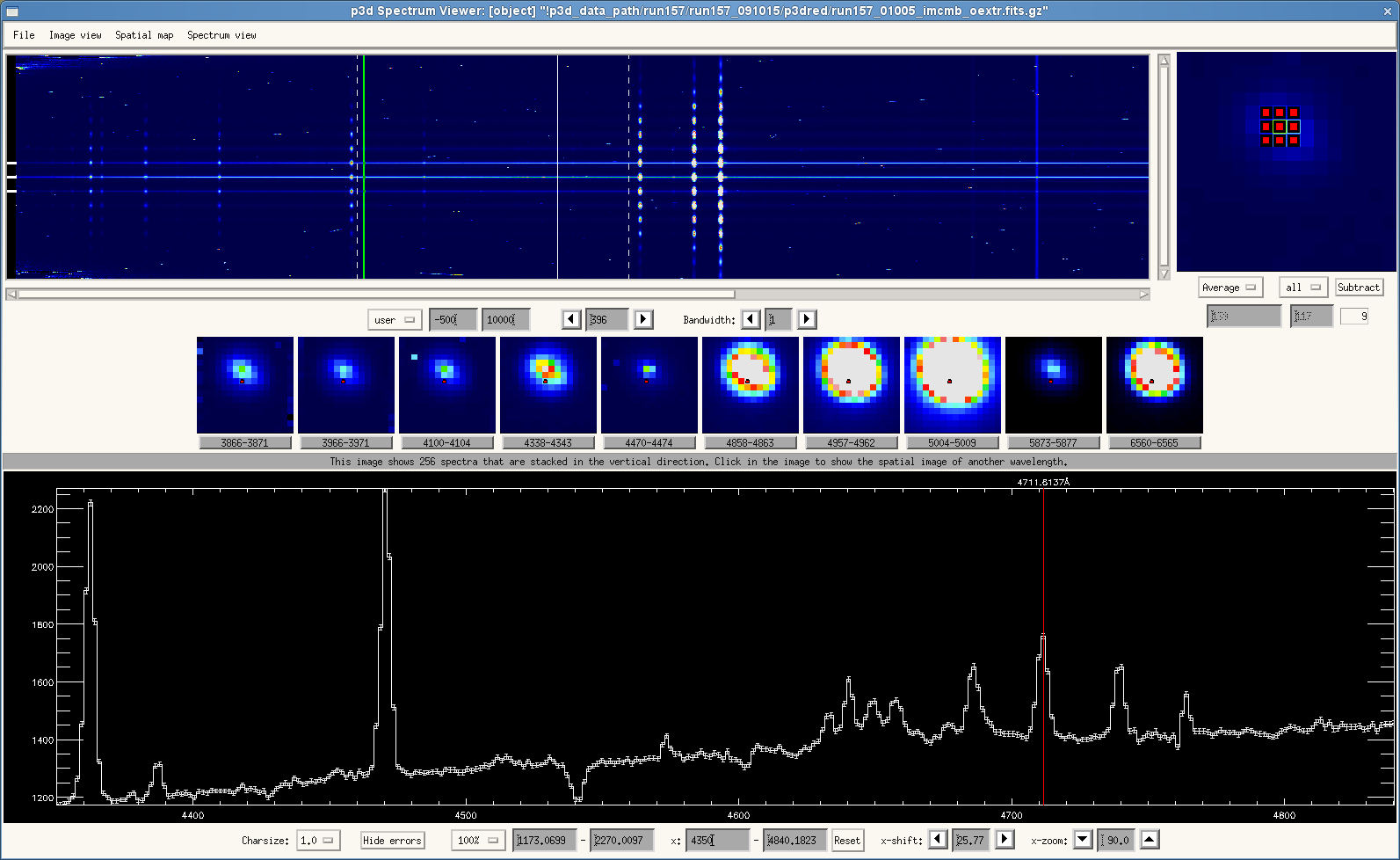
Figure 6: A screenshot of the p3d spectrum viewer for a planetary nebula. The different regions of the tool show the spectrum image (in the top-left region, cf. Fig. 7), a spatial map of a selected wavelength (in the top-right region, cf. Fig. 8), a set of ten stored spatial maps for ten wavelengths and a status line (middle region), and an average plot of the nine spectra that are selected in the spatial map (in the bottom region, cf. Fig. 9).

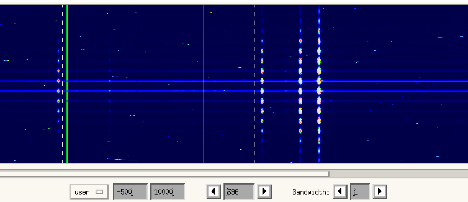
Figure 7: Each line in this image represents a spectrum. The brighter features, which are ordered vertically, represent emission lines of H$\gamma$, H$\beta$, and two forbidden lines of $O^{2+}$ ($[\mbox{O}\textsc{iii}]\,\lambda\lambda 4959,5007$). The brighter horizontal lines contain the central star continuum, and the randomly placed features are residuals of cosmic rays. The controls at the bottom allow to set the color cut levels, select the wavelength bin that is used to show the spatial map (the green vertical bar), and to define the width of the green bar.

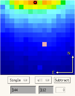
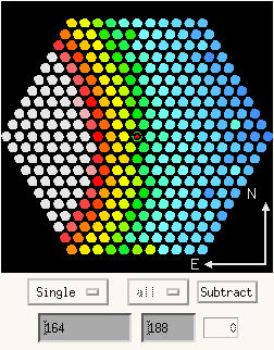
Figure 8: The spatial map presents an intensity image as it is seen on the sky. The left-hand (right-hand) side image shows one) selected spatial element, among all 256 (331) square-shaped (circular) spatial elements of the PMAS/LARR (PMAS/PPAK) IFU. The orientation of the IFU is also indicated, north is up and east to the left. The controls at the bottom show the spectrum id, among other things.

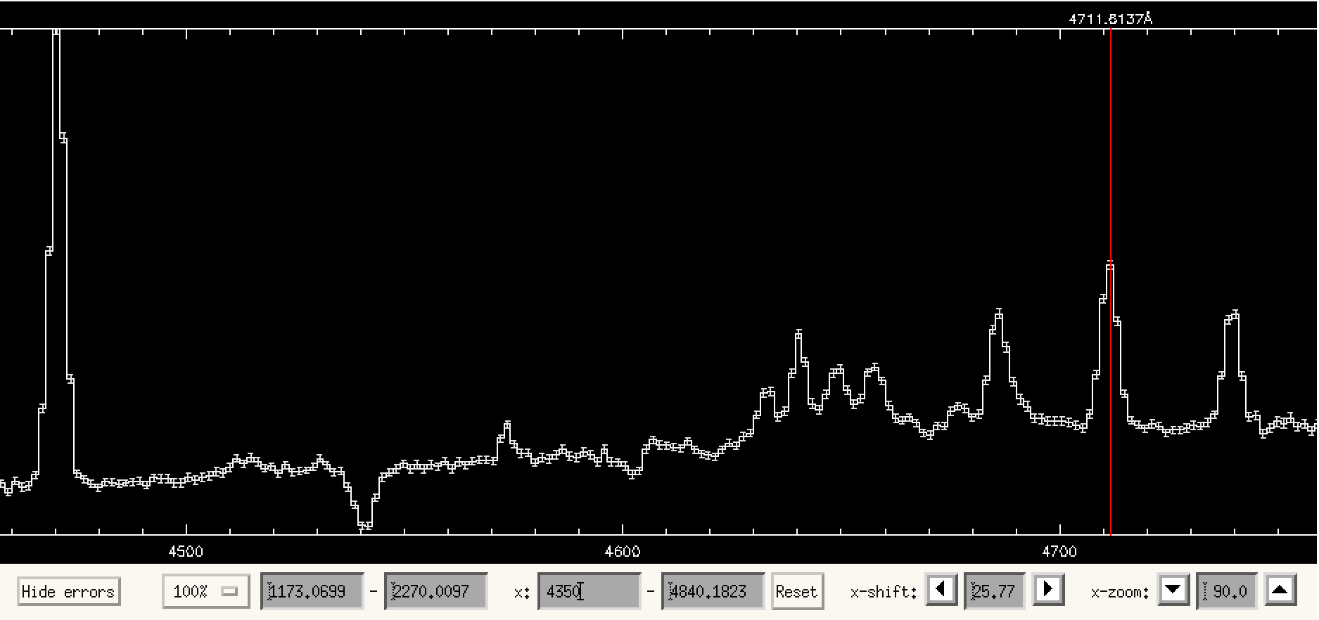
Figure 9: This image shows a section of the full wavelength range of the data for the selected spectrum, or, alternatively, of a set of averaged or summed spectra. Errors are shown with bars. The emission line at the cursor location, which is indicated with a red vertical line here (and simultaneously with a white vertical line in the spectrum image, Fig. 7) comes from a forbidden line of Ar³⁺. The controls at the bottom allow a quick change of the properties of the shown spectrum.

References

- Kissler-Patig et al. (2004) Kissler-Patig, M., Copin, Y., Ferruit, P., Pecontal-Rousset, A., Roth, M.M., 2004, AN 325, 159
- Roth (2010) Roth, M.M. 2010, in: 3D Spectroscopy for Astronomy, Lectures of the XVII. IAC Winterschool of Astrophysics, ed. E. Mediavilla, S. Arribas, M.M. Roth, J. Cepa-Nogue, F. Sanchez, Cambridge University Press, p.1
- Sandin et al. (2010) Sandin, C., Becker, T., Roth, M. M., Gerssen, J., Monreal-Ibero, A., Böhm, P., Weilbacher, P. 2010, A&A 515, 35
- Wells et al. (1981) Wells, D.C., Greisen, E.W., Harten, R.H. 1981, A&AS 44, 363