Analysis of the Disorder-Induced Zero Bias Anomaly in the Anderson-Hubbard Model

Abstract

Using a combination of numerical and analytical calculations, we study the disorder-induced zero bias anomaly (ZBA) in the density of states of strongly-correlated systems modeled by the two dimensional Anderson-Hubbard model. We find that the ZBA comes from the response of the nonlocal inelastic self-energy to the disorder potential, a result which has implications for theoretical approaches that retain only the local self-energy. Using an approximate analytic form for the self-energy, we derive an expression for the density of states of the two-site Anderson-Hubbard model. Our formalism reproduces the essential features of the ZBA, namely that the width is proportional to the hopping amplitude $t$ and is independent of the interaction strength and disorder potential.

I Introduction.

The Anderson-Hubbard model (AHM) is the simplest model that describes strongly-correlated electrons in a disordered lattice. The AHM is widely used, for example, to describe doped transition metal oxides, where the electronic properties are affected by both a strong local Coulomb repulsion and doping-related disorder.Imada et al. (1998) The AHM is also relevant to cold atomic gases in random optical lattices,Schneider et al. (2008); White et al. (2009); Zhou and Das Sarma (2010) and there has been recent interest in the AHM as a model interacting system that exhibits Anderson localization.Tusch and Logan (1993); Heidarian and Trivedi (2004); Byczuk et al. (2005); Kotlyar and Das Sarma (2001); Tanasković et al. (2003); Paris et al. (2007); Chakraborty et al. (2007); Song et al. (2008); Henseler et al. (2008a, b); Andrade et al. (2009); Byczuk et al. (2009); Pezzoli and Becca (2010); Semmler et al. (2010) The physics of the AHM is determined by dimensionality, by filling, and by the three energy scales: the kinetic energy $t$, the on-site Coulomb repulsion $U$, and the disorder strength $\Delta$. When $\Delta=0$, this model reduces to the well-known Hubbard model which, despite its simplicity, has only been solved exactly in the limits of oneLieb and Wu (1968) and infinite dimensionsGeorges et al. (1996).

In the Hubbard model, the interesting physics arises from a competition between $t$, which tends to delocalize electrons, and $U$, which tends to localize electrons. When the lattice is half filled (i.e. when there is one electron per site), a sufficiently large $U$ can generate a Mott insulating phase. The Mott transition occurs at a critical $U_{c}$ that depends on the details of the lattice. Much of the Hubbard model research in the past few decades has revolved around strong correlation effects slightly away from the Mott insulating phase, which is achieved either by taking $U$ less than $U_{c}$ or by doping away from half filling. One of the important ideas to come out of the Hubbard model is that the low energy physics of the strongly correlated metal phase near the Mott transition is governed by an effective interaction $J\sim t^{2}/U$.Dagotto (1994)

Contrary to this, recent exact diagonalization and quantum Monte Carlo studies of the two-dimensional Anderson-Hubbard model have found that a zero bias anomaly (ZBA) of width $t$ forms in the density of states (DOS).Chiesa et al. (2008) The ZBA appears as a V-shaped dip in the DOS at the Fermi energy $\varepsilon_{F}$, as shown in Fig. 1. While it is not surprising that disorder might introduce another low energy scale other than $t^{2}/U$, it is surprising that this new scale is independent of both $U$ and $\Delta$.

It is worth emphasizing that the observed ZBA is not explained by the conventional Altshuler-Aronov theory of weakly correlated metals. In Altshuler-Aronov theory, the magnitude of the ZBA depends inversely on a dimension-dependent power of the Fermi velocity,Altshuler and Aronov (1985) while the AHM ZBA grows linearly with the Fermi velocity (which is approximately $2t$).

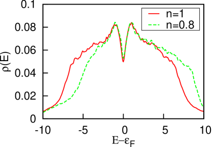
Figure 1: (color online) Density of states for electron densities $n=1$ (half filling) and $n=0.8$, showing the V-shaped zero bias anomaly at ${\varepsilon_{F}}$. Results are for exact diagonalization of 12 site lattices, and are averaged over 1000 disorder configurations. Model parameters are $\Delta=20t$ and $U=8t$ throughout this work, unless stated otherwise.

The physics of this ZBA is subtle, and is not captured by most approximations. The Hartree-Fock approximationTusch and Logan (1993); Heidarian and Trivedi (2004); Fazileh et al. (2006); Chen and Gooding (2009); Shinaoka and Imada (2009a); Shinaoka and Imada (2009b); Shinaoka and Imada (2010) yields a V-shaped zero bias anomaly when magnetic moments are allowed to form,Chen and Gooding (2009) and has a low-energy soft gap that is apparently associated with a multi-valley energy landscape.Shinaoka and Imada (2009b) However, the width of the ZBA grows with $U$, suggesting that the physics of the ZBA is different than that found by exact diagonalization. Furthermore, the evidence for a soft gap in exact diagonalization calculations is less well established,Shinaoka and Imada (2009b) and it is possible that quantum fluctuations fill in the soft gap. Another common approximation, dynamical mean field theory (DMFT),Ulmke et al. (1995); Miranda and Dobrosavljević (2005); Laad et al. (2001); Balzer and Potthoff (2005); Lombardo et al. (2006); Song et al. (2008); Andrade et al. (2009); Semmler et al. (2010) includes strong correlation physics, but has not found a ZBA at all. It has been arguedSong et al. (2009) that this is because of nonlocal contributions to the self-energy neglected in these calculations. Recent analytical studies of the two site AHM do find a ZBA with qualitative features that are consistent with exact diagonalization. These calculations interpret the ZBA in terms of level repulsion between many-body eigenstates,Wortis and Atkinson (2010); Chen and Atkinson (2010); Wortis and Atkinson and demonstrate how strong correlations can generate a kinetic energy driven ZBA. While these studies are instructive, it is difficult to connect them to the more usual language of many-body self-energies in interacting systems.

In this article, we show how the ZBA arises from the response of the inelastic self-energy to the disorder potential, using an approach that is loosely based on one used by Abrahams et al.Abrahams et al. (1981) to study the ZBA in weakly-correlated metals. We restrict ourselves to two dimensions, where the existence of the ZBA is well established, and work in the limit of strong disorder. In Sec. II.1, we show that the ZBA comes from nonlocal contributions to the local density of states, establishing (i) that the ZBA is not a remnant of the Mott gap and (ii) that approximations such as Hartree-Fock and DMFT (which retain only the local self-energy) are missing key nonlocal physics. In Sec. II.2, we discuss an approximate self-energy, based on equation-of-motion calculations,Song et al. (2009) which highlights the role of nonlocal spin and charge correlations. We show numerically that this approximation works well for large disorder, and then derive in Sec. II.3 an approximate expression for the density of states (DOS) based on this self-energy. We find that the energy $t$ appears as the natural energy scale for the ZBA. The results are summarized in Sec. III.

II Calculations

Before we proceed with the calculations, we emphasize a significant difference between weakly and strongly correlated systems that affects our analysis. In the atomic limit, obtained by setting $t=0$, the DOS is a sum of the local spectrum at each atomic site. For noninteracting systems, each local spectrum has a single resonance at the orbital energy $\epsilon$ of that site. However, for strongly correlated systems, there are two resonances, at $\epsilon$ and $\epsilon+U$, which we term the lower Hubbard orbital (LHO) and upper Hubbard orbital (UHO) respectively. These energies correspond to transitions in which an electron is added to a site that is initially empty (LHO) or singly occupied (UHO). The LHO and UHO are precursors of the lower and upper Hubbard bands that form when $t$ is nonzero.

The calculations in this work are based on an expansion around the atomic limit and are appropriate for the strong disorder case. By strong disorder, we mean $\Delta/2z\gg t$, where $z$ is the coordination number of the lattice and $\Delta/2z$ is of the order of the average level spacing of the $z$ sites adjacent to any site in the lattice, and the factor of 2 is because there is an LHO and a UHO at each site. In this limit, the local spectrum at a particular lattice site is dominated by $2(z+1)$ resonances associated with the site and its $z$ nearest neighbors.Song et al. (2008)

II.1 Analysis of Numerical Results

In this section, we develop a framework that explicitly shows the role of local and nonlocal correlations in the DOS. We then use this framework to analyze the results of numerical exact diagonalization calculations for the AHM. We begin with a brief description of the exact diagonalization calculations.

The AHM Hamiltonian is

$$\hat{H}=\sum_{i,j,\sigma}t_{ij}\hat{c}^{\dagger}_{i\sigma}\hat{c}_{j\sigma}+\sum_{i}\left(\epsilon_{i}\hat{n}_{i}+U\hat{n}_{i\uparrow}\hat{n}_{i\downarrow}\right),$$ (1)

where $t_{ij}=-t$ for nearest-neighbor sites $i$ and $j$, and is zero otherwise; $\hat{c}_{i\sigma}$ and $\hat{n}_{i\sigma}$ are the annihilation and number operators for lattice site $i$ and spin $\sigma$, and $\epsilon_{i}$ is the energy of the orbital at site $i$. Disorder is introduced by choosing $\epsilon_{i}$ from a uniform distribution $\epsilon_{i}\in[-\frac{\Delta}{2},\frac{\Delta}{2}]$.

The AHM can be solved exactly for small clusters. For our numerical work, we use a standard Lanczos methodDagotto (1994) to find the ground states of two-dimensional $N$-site ($N=10$, 12) clusters with periodic boundary conditions, and then use a block-recursion method to find the full nonlocal Green’s function $G_{ij}(\omega)$ for the lattice.Golub and van Loan (1996) The DOS is

$$\rho(E)=-\frac{1}{\pi N}\mbox{Im }\langle\sum_{i}G_{ii}(E)\rangle,$$ (2)

where $\langle\ldots\rangle$ indicates an average over disorder configurations at fixed chemical potential. Examples of the disorder-averaged DOS are shown in Fig. 1.

The goal of this section is to relate the DOS to two physically interesting quantities, the local inelastic self-energy $\Sigma_{ii}(\omega)$ and the nonlocal hybridization function $\Lambda_{i}(\omega)$. For a given disorder configuration, the inelastic self energy is

$${\bf\Sigma}(\omega)={\bf G}_{0}(\omega)^{-1}-{\bf G}(\omega)^{-1},$$ (3)

where $(\ldots)^{-1}$ is a matrix inverse, ${\bf G}_{0}(\omega)$ is the noninteracting Green’s function for the same disorder configuration as ${\bf G}(\omega)$, and $\Sigma_{ii}(\omega)$ is a diagonal matrix element of ${\bf\Sigma}(\omega)$ (bold symbols indicate matrices in the space of lattice sites). The hybridization function is then defined by

$$G_{ii}(\omega)=[\omega-\epsilon_{i}-\Sigma_{ii}(\omega)-\Lambda_{i}(\omega)]^{-1},$$ (4)

where $G_{ii}(\omega)$ is the local Green’s function at site $i$, and $\Sigma_{ii}$ is a diagonal matrix element of ${\bf\Sigma}(\omega)$. Both $\Sigma_{ii}(\omega)$ and $\Lambda_{i}(\omega)$ can be extracted from our numerical calculations: Eq. (3) gives $\Sigma_{ii}(\omega)$, and then Eq. (4) can be inverted to find $\Lambda_{i}(\omega)$.

In the following analysis, we derive a formal expression for $\rho(E)$ in terms of $\Sigma_{ii}(\omega)$ and $\Lambda_{i}(\omega)$. Our starting point is Eq. (2), with $G_{ii}(\omega)$ given by Eq. (4). It is clear from these two equations that $\rho(E)$ depends directly on $\Sigma_{ii}(\omega)$ and $\Lambda_{i}(\omega)$, and the main issue we face in our derivation is how to perform the disorder average in Eq. (2). We do this in two steps: first, we take a partial disorder average of $\Sigma_{ii}(\omega)$ and $\Lambda_{i}(\omega)$ over $\epsilon_{j}$ for $j\neq i$ and for fixed $\epsilon_{i}$; second, we average $G_{\epsilon_{i}}(\omega)$ over $\epsilon_{i}$. As a result of the first averaging process,

$$S_{i}\rightarrow S_{\epsilon}=\langle S_{i}\delta(\epsilon-\epsilon_{i})\rangle$$ (5)

where $S_{i}(\omega)=\Sigma_{ii}(\omega)+\Lambda_{i}(\omega)$. This gives the average self-energy of all sites with energy $\epsilon$. Then

$$G_{\epsilon}(\omega)\approx[\omega-\epsilon-S_{\epsilon}(\omega)]^{-1}.$$ (6)

Equation (5) is the main approximation made in our derivation, and we check below that we do not lose the physics of the ZBA as a result of it. The next step is to average $G_{\epsilon}(\omega)$ over the local site energy.

To perform this average, we expand $S_{\epsilon}(\omega)$ about an energy $E$ near $\varepsilon_{F}$, by analogy to what is done in Fermi liquid theory. In making this expansion, we consider two categories of site: (i) sites with $\epsilon\sim E$ (LHO near $E$) and (ii) sites with $\epsilon+U\sim E$ (UHO near $E$). Sites with neither $\epsilon$ nor $\epsilon+U$ near $E$ do not contribute to the DOS at $E$ and are not included in our calculations. For cases (i) and (ii)

$$S_{\epsilon}(\omega) \approx S_{\overline{E}}(E)+(\epsilon-\overline{E})\partial_{\epsilon}S_{\epsilon}(E)_{\epsilon=\overline{E}}$$ (7)

$$+(\omega-E)\partial_{\omega}S_{\overline{E}}(\omega)_{\omega=E}$$

where $\overline{E}=E$ for case (i) and $\overline{E}=E-U$ for case (ii). Then the local Green’s function for site energy $\epsilon$ is

$$G_{\epsilon}(\omega)\approx\frac{Z}{\omega-E-(\epsilon-{\overline{E}})/m^{\ast}-Z[S_{\overline{E}}(E)-\overline{U}]}$$ (8)

with $Z=[1-\partial_{\omega}S_{\overline{E}}(\omega)]_{\omega=E}^{-1}$, ${m^{\ast}}^{-1}=Z{[1+\partial_{\epsilon}S_{\epsilon}(E)]_{\epsilon={\overline{E}}}}$, and $\overline{U}=E-\overline{E}$. The final term in the denominator, $S_{\overline{E}}(E)-\overline{U}$, vanishes identically in the atomic limit (Appendix A). Near the atomic limit, $S_{\epsilon}(\omega)$ is complex, with small real and imaginary parts that shift and broaden the orbital energies. We show in Sec. II.2 that the imaginary part of $S_{\epsilon}(E)$, which results from disorder averaging, is of order $zt^{2}/\Delta$.

Because the imaginary part of $S_{\epsilon}(E)$ is small, the average of $G_{\epsilon}(E)$ over $\epsilon$ is easily done (Appendix B), and we obtain the DOS

$$\rho(E) = -\frac{\mbox{Im }}{\pi\Delta}\int_{-\Delta/2}^{\Delta/2}G_{\epsilon}(E)d\epsilon$$ (9)

$$= \frac{1}{\Delta}\left[\frac{1}{1+\partial S_{\mathrm{LHO}}(E)}+\frac{1}{1+\partial S_{\mathrm{UHO}}(E)}\right],$$

where we have adopted the convenient notation

$$\partial S_{\mathrm{LHO}}(E) \equiv \mbox{Re }\partial_{\epsilon}S_{\epsilon}(E)|_{\epsilon=E}$$

$$\partial S_{\mathrm{UHO}}(E) \equiv \mbox{Re }\partial_{\epsilon}S_{\epsilon}(E)|_{\epsilon=E-U}.$$

The two terms in the sum in Eq. (9) give the partial DOS for the LHO and UHO. For each term, there are two distinct contributions: the first, $\partial_{\epsilon}\Sigma_{\epsilon}(E)$, includes local Mott physics; the second, $\partial_{\epsilon}\Lambda_{\epsilon}(E)$, includes the effects of nonlocal self-energies. Equation (9) is exact in the atomic limit (Appendix A), and is a good approximation for large disorder, where the imaginary part of $S_{\epsilon}(E)$ is small and independent of $E$ (see Appendix B). equation is derived assuming $U<U_{c}$, where $U_{c}\approx\Delta$ in the large disorder limit, since the system is a gapped Mott insulator for $U>U_{c}$.

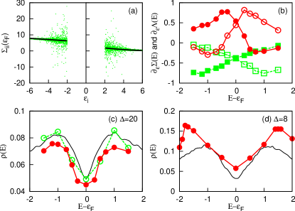
Figure 2: (color online) Origin of the zero bias anomaly. Data are for $n=1$, $U=8$, $\Delta=20t$, $t=1$, unless otherwise indicated. (a) $\Sigma_{\epsilon_{i}}(E)$ for $E=\varepsilon_{F}=U/2$ versus site energy $\epsilon_{i}$. Data is shown for sites with $\epsilon_{i}+U\approx E$ (left) and $\epsilon_{i}\approx E$ (right). Lines are quadratic least-squares fits to the data in each region and are used to determine $\partial_{\epsilon}\Sigma_{\epsilon}(E)$; (b) $\partial_{\epsilon}\Sigma_{\epsilon}(E)|_{\epsilon=\overline{E}}$ (squares) and $\partial_{\epsilon}\Lambda_{\epsilon}(E)|_{\epsilon=\overline{E}}$ (circles) for $\overline{E}=E$ (solid symbols) and $\overline{E}=E-U$ (empty symbols). (c) The approximate DOS, calculated using the results from (b) in Eq. (9) (solid circles), the exact DOS (solid line), and the DOS for the approximate self-energy (14) (empty circles). (d) Results of a similar analysis for $\Delta=8$.

Equation (9) gives an explicit relation between $\rho(E)$ and the functions $\Sigma_{\epsilon}(\omega)$ and $\Lambda_{\epsilon}(\omega)$. One can interpret the derivatives $\partial_{\epsilon}\Sigma_{\epsilon}(\omega)$ and $\partial_{\epsilon}\Lambda_{\epsilon}(\omega)$ as the response of the self-energy and hybridization function to changes in the local potential or, equivalently, the response of these functions to the disorder potential. This is reminiscent of the situation in weakly correlated metals, where a similar analysis related the ZBA to the response of the charge density to the disorder potential.Abrahams et al. (1981)

We use Eq. (9), in conjunction with our numerical calculations, to establish the relative importance of $\Lambda_{i}(\omega)$ and $\Sigma_{ii}(\omega)$ in forming the ZBA. The first step is to extract $\partial_{\epsilon}\Sigma_{\epsilon}(\omega)$ and $\partial_{\epsilon}\Lambda_{\epsilon}(\omega)$ from numerics. This process is illustrated in Fig. 2. For a given disorder configuration, $\Sigma_{ii}(E)$ is calculated from Eq. (3) at a fixed value of $E$, chosen to be ${\varepsilon_{F}}$ in Fig. 2. (Note that, for a finite size lattice, both $\Lambda_{i}(\omega)$ and $\Sigma_{ii}(\omega)$ are real.) The collected values of $\Sigma_{ii}(E)$ for all sites $i$ and for 1000 configurations are shown in Fig. 2(a). Data is shown for the two ranges, $\epsilon_{i}+U\approx\varepsilon_{F}$ and $\epsilon_{i}\approx\varepsilon_{F}$, that contribute to $\rho(\varepsilon_{F})$. A disorder-averaged $\Sigma_{\epsilon}(E)$ is found by making least-squares quadratic fits to the data in each range, from which the derivatives $\partial_{\epsilon}\Sigma_{\epsilon}(\varepsilon_{F})_{\epsilon=\varepsilon_{F}}$ and $\partial_{\epsilon}\Sigma_{\epsilon}(\varepsilon_{F})_{\epsilon=\varepsilon_{F}-U}$ are extracted. An identical set of calculations is then made for $\partial_{\epsilon}\Lambda_{\epsilon}(\varepsilon_{F})$. The calculations are repeated for other values of $E$, and resulting derivatives are plotted as functions of $E$ in Fig. 2(b).

As a check, we compare in Fig. 2(c) the DOS from Eq. (9), calculated using the values shown in Fig. 2(b), with the exact DOS. The agreement between the two is very good. We have repeated this analysis for other values of $\Delta$, and continue to find qualitative agreement down to the Mott transition at $\Delta\approx U$ [Fig. 2(d)].

Figure 2(b) shows the relative contributions to the ZBA made by $\Sigma_{ii}(\omega)$ and $\Lambda_{i}(\omega)$. The figure shows that $\partial_{\epsilon}\Sigma_{\epsilon}(E)_{\epsilon=\overline{E}}$ is negative for both LHO ($\overline{E}=E$) and UHO ($\overline{E}=E-U$). From Eq. (9), we see that a negative derivative corresponds to an increase in $\rho(E)$, and not to the V-shaped suppression of the DOS required to form a ZBA. This result demonstrates that the ZBA does not come from the local self-energy, and is therefore not a remnant of the Mott gap. More significantly, it demonstrates that the physics underlying the ZBA cannot be reproduced by approximations that include only the local self-energy, such as single-site DMFT or the Hartree-Fock approximation. The ZBA that appears in unrestricted Hartree-Fock calculations must have a different origin than that found here.

In contrast to the self-energy derivative, $\partial_{\epsilon}\Lambda_{\epsilon}(E)_{\epsilon=\overline{E}}$ is positive for $E\approx\varepsilon_{F}$ and negative away from $\varepsilon_{F}$, indicating that interorbital hybridization shifts spectral weight away from $\varepsilon_{F}$. This shows that the ZBA comes from nonlocal correlations embedded in the hybridization function. On the one hand, this is not surprising since the Hubbard model in low dimensions is known to map onto effective models with nonlocal interactions; on the other hand, the energy scale $t$ of the ZBA is not consistent with the energy scale $t^{2}/U$ of these effective models.

We note one further interesting feature of Fig. 2(b): the plots of $\partial_{\epsilon}\Lambda_{\epsilon}(E)_{\epsilon=E}$ and $\partial_{\epsilon}\Lambda_{\epsilon}(E)_{\epsilon=E-U}$ are asymmetric with respect to $\varepsilon_{F}$. This asymmetry indicates that LHOs and UHOs behave differently when they are below or above $\varepsilon_{F}$. We will return to this point below.

In summary, we have established two main results in this section. First, we have developed an expression, Eq. (9), for the DOS that relates $\rho(E)$ to the response of $\Sigma_{\epsilon}(E)$ and $\Lambda_{\epsilon}(E)$ to the disorder potential. Second, we have used this expression to analyze exact diagonalization results, and have shown that the ZBA is the result of nonlocal correlations, rather than the local self-energy.

II.2 Structure of the Hybridization Function

In the previous section, we established that the ZBA can be related to the derivative of $\Lambda_{\epsilon}(\omega)$ with respect to the site energy $\epsilon$. In this section, we analyse the structure of $\Lambda_{\epsilon}(\omega)$ in more detail in order to see the role of spin and charge fluctuations in forming the ZBA.

We begin by writing $\Lambda_{i}(\omega)$ in terms of an alternative exact expressionGeorges et al. (1996) that is more transparent than the original definition [Eq. (4)]:

$$\Lambda_{i}(\omega)=\sum_{j,k\neq i}[t_{ij}+\Sigma_{ij}(\omega)]G_{jk}^{{i\kern-2.10002pt/}}(\omega)[t_{ki}+\Sigma_{ki}(\omega)],$$ (10)

where $G_{jk}^{{i\kern-2.10002pt/}}(\omega)$ is a Green’s function matrix element for the lattice with site $i$ removed.Gfn This equation shows explicitly how the matrix elements $t_{ij}+\Sigma_{ij}(\omega)$ couple the site $i$ to the rest of the lattice. In general, $G_{jk}^{{i\kern-2.10002pt/}}(\omega)$ is not trivial to calculate, and this expression is of use only when $G_{jk}^{i\kern-2.10002pt/}(\omega)$ can be simplified through some approximation or limit. Here, we are in the limit of large disorder and low dimension, for which $G_{jk}^{{i\kern-2.10002pt/}}(\omega)$ is approximately local. In our discussion, we thus consider only the dominant contributions, with $j=k$, in the sum in Eq. (10):

$$\Lambda_{i}(\omega)\approx\sum_{j\in\mathrm{nn}_{i}}[-t+\Sigma_{ij}(\omega)]^{2}G_{jj}^{{i\kern-2.10002pt/}}(\omega),$$ (11)

where $j\in\mathrm{nn}_{i}$ indicates that $j$ is a nearest neighbor of $i$.

We note that, while $\Lambda_{i}(\omega)$ is real for a single disorder configuration on a finite lattice, the disorder-averaged hybridization function $\Lambda_{\epsilon}(\omega)$ is complex. The real part of $\Lambda_{\epsilon}(\omega)$ describes shifts of the LHO and UHO energies while the imaginary part describes the broadening of these orbitals due to the lattice. For the analysis in this work to make sense, the broadening must be much less than the level spacing ($\sim\Delta/2z$) of the local spectrum, so that discrete energy levels at each site keep their distinct identity. We can estimate the broadening from a simplified disorder average of Eq. (11). Setting $\Sigma_{ij}=0$, we obtain

$$\Lambda^{0}_{\epsilon_{i}}(\omega) = zt^{2}\langle G_{jj}^{{i\kern-2.10002pt/}}(\omega)\rangle_{j},$$ (12)

where the sum over $j$ is replaced by the factor $z$, and $\langle\ldots\rangle_{j}=\Delta^{-1}\int_{-\Delta/2}^{\Delta/2}\ldots d\epsilon_{j}$ is the disorder average over site $j$. This equation assumes that $G_{jj}^{i\kern-2.10002pt/}(\omega)$ with different $j$ are independent of each other. The imaginary part of Eq. (12) is

$$\mbox{Im }\Lambda^{0}_{\epsilon_{i}}(\omega) \approx -\pi zt^{2}\rho(\omega)\sim-\frac{3z\pi t^{2}}{2\Delta},$$ (13)

which gives a broadening of $O(zt^{2}/\Delta)$. The condition that this is much less than the level spacing of the local spectrum can be written $2z^{2}t^{2}/\Delta^{2}\ll 1$, which is met provided our initial assumption $2zt/\Delta\ll 1$ is met.

Equation (11) shows that the nonlocal self-energy is central to the ZBA. To proceed further, we need an analytic form for this self-energy, and we adopt a partial fractions expansion for the self-energy that is based on the equation-of-motion method.Song et al. (2009) The rationale for this choice is that the equation-of-motion method correctly reproduces the LHO and UHO in the atomic limit, and has been shown to be accurate for the two-site AHM.Song et al. (2009) In general, we expect this method to work well when short-range physics dominates. The nonlocal self energy has the form

$$\Sigma_{ij}(\omega)=\frac{-tU^{2}p_{ij}}{(\omega-\epsilon_{i\sigma}-Uh_{i{\overline{\sigma}}})(\omega-\epsilon_{j\sigma}-Uh_{j{\overline{\sigma}}})-\frac{\displaystyle O(t^{2})}{\displaystyle\omega-\ldots}},$$

(14)

where we suppress the explicit dependence of $\Sigma_{ij}(\omega)$ and $p_{ij}$ on $\sigma$ because we are considering only nonmagnetic phases, where $h_{i{\overline{\sigma}}}=1-n_{i{\overline{\sigma}}}$, $n_{i{\overline{\sigma}}}=\langle\hat{n}_{i{\overline{\sigma}}}\rangle$, with ${\overline{\sigma}}=-\sigma$, and where

$$p_{ij}=\langle\delta\hat{n}_{i{\overline{\sigma}}}\delta\hat{n}_{j{\overline{\sigma}}}\rangle+\langle\hat{S}_{i+}\hat{S}_{j-}\rangle-\langle\hat{D}_{i}^{\dagger}\hat{D}_{j}\rangle.$$ (15)

(Here, $\langle\ldots\rangle$ indicates the expectation value, rather than the disorder average.) The three nonlocal correlations making up $p_{ij}$ involve density fluctuation operators $\delta\hat{n}_{i\sigma}=\hat{n}_{i\sigma}-n_{i\sigma}$, spin-flip operators $\hat{S}_{i\pm}$, and pair annihilation operators $\hat{D}_{i}=c_{i\downarrow}c_{i\uparrow}$. The last of these three is an order of magnitude smaller than the other terms and is discarded for the remaining discussion.

In general, the usefulness of Eq. (14) is limited by the difficulty of finding the higher-order terms in the continued fraction. These terms are important for determining the pole structure of the self-energy, but do not change the fact that $\Sigma_{ij}\propto p_{ij}$. In the disorder-free Hubbard model, it has been shown that these higher order terms are qualitatively important;Odashima et al. (2005) however, the strongly disordered case is close to the atomic limit and may be understood qualitatively through a truncated self-energy, obtained by dropping the $O(t^{2})$ term in (14). We check this assertion numerically: we calculate an approximate $\Lambda_{i}(\omega)$ using the self-energy (14) in Eq. (11), and then calculate an approximate DOS using Eq. (9). The results are plotted in Fig. 2(c) in comparison with exact diagonalization calculations, and the agreement between the two is good.

We showed in the previous section that the ZBA comes from the response of $\Lambda_{\epsilon}(E)$ to the disorder potential via the derivative $\partial_{\epsilon}\Lambda_{\epsilon}(E)$. The main idea suggested by Eqs. (11) and (14) is that this response is directly related to the response of $\Sigma_{ij}(E)$, and therefore of $p_{ij}$, to the disorder potential. We show in the next section that there are other contributions, but that a large part of the ZBA can indeed be traced back to the response of the nonlocal charge and spin correlation functions to the disorder potential.

We note that the form of $\Sigma_{ij}(\omega)$ explains the asymmetry in $\partial_{\epsilon}\Lambda_{\epsilon}(E)_{\epsilon=E}$ and $\partial_{\epsilon}\Lambda_{\epsilon}(E)_{\epsilon=E-U}$ with respect to ${\varepsilon_{F}}$, shown in Fig. 2(b). This figure shows that the ZBA is formed from a shift away from ${\varepsilon_{F}}$ of LHOs below ${\varepsilon_{F}}$ and of UHOs above ${\varepsilon_{F}}$. According to Eq. (14), this asymmetric shift occurs because the correlation $p_{ij}$ is largest when sites $i$ and $j$ are both singly-occupied, namely when ${\varepsilon_{F}}-U\lesssim\epsilon_{i},\epsilon_{j}\lesssim{\varepsilon_{F}}$. (The spin correlations vanish when either site is empty or doubly occupied.) This condition on $\epsilon_{i}$ and $\epsilon_{j}$ is equivalent to the requirement, at each site, that the LHO be below ${\varepsilon_{F}}$ and the UHO be above ${\varepsilon_{F}}$.

In summary, we have used a form for the hybridization function that shows explicitly the role of the nonlocal self-energy. We have proposed using an analytic form, Eq. (14), for this self-energy, and have shown numerically that it reproduces the density of states obtained by exact diagonalization. The main result of this section is that the nonlocal self-energy, and therefore the ZBA, depends on nonlocal spin and charge correlations.

Ideally, one would now like to use this formalism to derive an analytic expression for the density of states; this requires knowledge of $p_{ij}$ and is in general quite difficult since $p_{ij}$ is different along every bond in the lattice. In the next section, we therefore focus on a simple model for which $p_{ij}$ is known, and the DOS can be found analytically.

II.3 Density of States

As a simple application of the formalism derived in the previous sections, we calculate the DOS for the two-site AHM (2SAHM). This model has been studied elsewhere by direct diagonalization of the Hamiltonian,Wortis and Atkinson (2010); Chen and Atkinson (2010); Wortis and Atkinson and provides a point of comparison for the current work. Our approach is straightforward: we use the self-energy (14) to find an approximate hybridization function with which we evaluate the density of states using Eq. (9).

The 2SAHM consists of an ensemble of two-atom “molecules” with random site energies $\epsilon_{i}$ and $\epsilon_{j}$. The disorder averaged hybridization function for site $i$ is

$$\Lambda_{\epsilon_{i}}(\omega)=\langle[-t+\Sigma_{ij}(\omega)]^{2}G_{jj}^{{i\kern-2.10002pt/}}(\omega)\rangle_{j}.$$ (16)

In this form, the hybridization function has a useful symmetry (Appendix D)

$$\partial\Lambda_{\mathrm{UHO}}({\varepsilon_{F}}+\tilde{E})=\partial\Lambda_{\mathrm{LHO}}({\varepsilon_{F}}-\tilde{E}),$$ (17)

where $\partial\Lambda_{\mathrm{LHO}}(E)$ and $\partial\Lambda_{\mathrm{UHO}}(E)$ have similar definitions as $\partial S_{\mathrm{LHO}}(E)$ and $\partial S_{\mathrm{UHO}}(E)$, and $\tilde{E}$ is the energy $E$ measured relative to ${\varepsilon_{F}}$.

One consequence of this symmetry is that contributions to $\partial\Lambda_{\mathrm{LHO}}(E)$ that are even under $\tilde{E}\rightarrow-\tilde{E}$ are more important for the ZBA than those which are odd. To show this, we define $\delta\rho(E)$ to be the change in the DOS due to the hybridization function, namely $\delta\rho(E)=\rho(E)-\rho_{0}(E)$, where $\rho_{0}(E)$ is evaluated with $\partial_{\epsilon}\Lambda_{\epsilon}(E)$ set to zero. To linear order in $\partial_{\epsilon}\Lambda_{\epsilon}(E)$, Eq. (9) gives

$$\delta\rho(E) = -\frac{1}{\Delta}\left[\frac{\partial\Lambda_{\mathrm{LHO}}(E)}{[1+\partial\Sigma_{\mathrm{LHO}}(E)]^{2}}+\frac{\partial\Lambda_{\mathrm{UHO}}(E)}{[1+\partial\Sigma_{\mathrm{UHO}}(E)]^{2}}\right].$$

Noting, from Fig. 2(b), that $\partial\Sigma_{\mathrm{LHO}}(E)\approx\partial\Sigma_{\mathrm{UHO}}(E)$ near ${\varepsilon_{F}}$, we get

$$\delta\rho(E)\sim-\frac{1}{\Delta}\frac{\partial\Lambda_{\mathrm{LHO}}(E)+\partial\Lambda_{\mathrm{UHO}}(E)}{[1+\partial\Sigma({\varepsilon_{F}})]^{2}}.$$ (19)

From this, and from Eq. (17), it follows that the most significant contributions to $\delta\rho(E)$ come from terms in $\partial\Lambda_{\mathrm{LHO}}(E)$ that are even in $\tilde{E}$.

To calculate $\partial\Lambda_{\mathrm{LHO}}(E)$, we expand Eq. (16) as $\Lambda_{\epsilon}(\omega)=\Lambda^{0}_{\epsilon}(\omega)+\Lambda^{\prime}_{\epsilon}(\omega)+\Lambda^{\prime\prime}_{\epsilon}(\omega)$, where

$$\Lambda^{0}_{\epsilon_{i}}(\omega) = t^{2}\langle G^{i\kern-2.10002pt/}_{jj}(\omega)\rangle_{j}$$ (20)

$$\Lambda^{\prime}_{\epsilon_{i}}(\omega) = -2t\langle\Sigma_{ij}(\omega)G^{i\kern-2.10002pt/}_{jj}(\omega)\rangle_{j}$$ (21)

$$\Lambda^{\prime\prime}_{\epsilon_{i}}(\omega) = \langle\Sigma_{ij}(\omega)^{2}G^{i\kern-2.10002pt/}_{jj}(\omega)\rangle_{j}.$$ (22)

We have evaluated each of these terms analytically and find that, by far, the largest contribution to the ZBA comes from $\partial\Lambda^{\prime\prime}_{\mathrm{LHO}}(E)$. In particular, $\partial\Lambda^{0}_{\mathrm{LHO}}(E)$ is an odd function of $\tilde{E}$ and therefore makes almost no contribution to the ZBA; $\partial\Lambda^{\prime}_{\mathrm{LHO}}(E)$ contains both odd and even terms and therefore does contribute to the ZBA, but is an order of magnitude smaller than $\partial\Lambda^{\prime\prime}_{\mathrm{LHO}}(E)$. It is, perhaps, not surprising that the term containing the highest power of $\Sigma_{ij}(\omega)$ makes the largest contribution to the ZBA. For clarity, we include only results for $\Lambda^{\prime\prime}_{\epsilon_{i}}(E)$ in our calculation of $\delta\rho(E)$.

Using Eq. (37) for $G_{jj}^{i\kern-2.10002pt/}(\omega)$, we obtain

$$\Lambda^{\prime\prime}_{\epsilon_{i}}(\omega) = \frac{t^{2}U^{4}}{\Delta}\int_{-\Delta/2}^{\Delta/2}d\epsilon_{j}\frac{p_{ij}^{2}}{(\omega-\epsilon_{i}-Uh_{i{\overline{\sigma}}})^{2}(\omega-\epsilon_{j}-Uh_{j{\overline{\sigma}}})(\omega-\epsilon_{j})(\omega-\epsilon_{j}-U)},$$ (23)

and differentiating this with respect to $\epsilon_{i}$, we obtain

$$\frac{\partial\Lambda_{\epsilon_{i}}^{\prime\prime}(\omega)}{\partial\epsilon_{i}} = \frac{t^{2}U^{4}}{\Delta}\int_{-\Delta/2}^{\Delta/2}d\epsilon_{j}\left[\partial_{\epsilon_{i}}p_{ij}^{2}+\frac{2p_{ij}^{2}(1+U\partial_{\epsilon_{i}}h_{i{\overline{\sigma}}})}{(\omega-\epsilon_{i}-Uh_{i{\overline{\sigma}}})}+\frac{p_{ij}^{2}U\partial_{\epsilon_{i}}h_{j{\overline{\sigma}}}}{(\omega-\epsilon_{j}-Uh_{j{\overline{\sigma}}})}\right]$$ (24)

$$\times\frac{1}{(\omega-\epsilon_{i}-Uh_{i{\overline{\sigma}}})^{2}(\omega-\epsilon_{j}-Uh_{j{\overline{\sigma}}})(\omega-\epsilon_{j})(\omega-\epsilon_{j}-U)}$$

To calculate $\partial\Lambda^{\prime}_{\mathrm{LHO}}(E)$, we set $\omega=\epsilon_{i}=E$ in Eq. (24). Then there are four terms, proportional to $\partial_{\epsilon_{i}}p_{ij}^{2}$, to $p_{ij}^{2}\partial_{\epsilon_{i}}h_{i{\overline{\sigma}}}$, to $p_{ij}^{2}\partial_{\epsilon_{i}}h_{j{\overline{\sigma}}}$, and to $p_{ij}^{2}$. The last of these is a factor $t/U$ smaller than the others and is discarded.

Because of the simplicity of the 2SAHM, we can write the coefficients $p_{ij}$, $h_{i{\overline{\sigma}}}$, and $h_{j{\overline{\sigma}}}$ in terms of the many-body wavefunction for the two site system, and thus find their explicit dependence on $\epsilon_{i}$ and $\epsilon_{j}$. This makes the integration over $\epsilon_{j}$ possible. The calculations are complicated by the fact that we do the integration at fixed chemical potential, meaning that the number of electrons in the ground state depends on $\epsilon_{i}$ and $\epsilon_{j}$. The dominant contribution to the ZBA comes from cases where the ground state has two electrons, and we include only this term in our result. The calculations are somewhat lengthy, and we leave the details to Appendix C.

The result of these calculations is, from Eq. (19) and Eq. (LABEL:a:dosdprime),

$$\delta\rho(E) \approx \frac{-28\sqrt{2}t}{27\Delta^{2}(1+\partial\Sigma)^{2}}\left[F_{2}(x)+F_{4}(x)+\frac{3\pi}{4}\right]$$ (25)

where $x=(2t^{2}-\tilde{E}^{2})/(2\sqrt{2}t|\tilde{E}|)$, with $\tilde{E}=E-{\varepsilon_{F}}$ and

$$F_{2}(x) = \frac{x}{x^{2}+1}+\tan^{-1}(x),$$

$$F_{4}(x) = \frac{1}{2}F_{2}(x)-\frac{x}{(x^{2}+1)^{2}}.$$

Equation (25) is plotted in Fig. 3 for the case $\Delta=20t$. For this plot, the unknown prefactor $1+\partial\Sigma$ is taken to be $0.7$, based on the value of $\partial_{\epsilon}\Sigma_{\epsilon}(E)|_{\epsilon={\varepsilon_{F}}}$ in Fig. 2(b). The resulting plot is qualitatively consistent with exact results for the 2SAHMWortis and Atkinson (2010); Chen and Atkinson (2010); from Eq. (25), the width of the ZBA is of order $2\sqrt{2}t$, and the depth is proportional to $t/\Delta^{2}$.

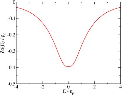
Figure 3: Theoretical density of states from Eq. (25). Results are shown for $\Delta/t=20$. Note that the curve is independent of $U$.

In previous studies of the 2SAHM, the ZBA was attributed to level repulsion between many-body states. Here, level repulsion is implicit in $\partial\Lambda_{\mathrm{LHO}}(E)$ and $\partial\Lambda_{\mathrm{UHO}}(E)$, since these describe the shifts of the atomic LHO and UHO due to neighboring sites. These shifts are primarily due to the response $\partial_{\epsilon_{i}}\Sigma_{ij}(E)$ of the nonlocal self-energy to the disorder potential. In Eq. (24), we showed that $\partial_{\epsilon_{i}}\Sigma_{ij}(E)$ depends on the local charge susceptibilities $\partial_{\epsilon_{i}}h_{i{\overline{\sigma}}}$ and $\partial_{\epsilon_{i}}h_{j{\overline{\sigma}}}$, and a generalized susceptibility $\partial_{\epsilon_{i}}p_{ij}$. For the 2SAHM, the last term is the largest, so that the ZBA is mostly due to the response of the nonlocal spin and charge correlation functions making up $p_{ij}$.

It is interesting to note that Mott physics suppresses this response. This is because the local Coulomb interaction tends to fix the charge density at each site, so that the spin and charge correlations are only weak functions of $\epsilon_{i}$. For example, configurations in which $\epsilon_{i}$ and $\epsilon_{j}$ are near ${\varepsilon_{F}}$ have a singlet ground state $|s\rangle$, with corrections of order $t/U$. A small change in $\epsilon_{i}$ changes this ground state, and therefore $p_{ij}$, by order $t/U$. Thus $\partial_{\epsilon_{i}}p_{ij}$ is suppressed by Mott physics. This is not the case when $\epsilon_{i}$ and $\epsilon_{j}+U$ are within $t$ of ${\varepsilon_{F}}$. Then $|s\rangle$ and $|02\rangle$ are nearly degenerate, and the proportions of $|s\rangle$ and $|02\rangle$ making up the ground state vary linearly with $\epsilon_{i}$. In this regime, $\partial_{\epsilon_{i}}p_{ij}$ is not small. The ZBA therefore comes from disorder configurations in which Mott physics does not suppress nonlocal charge fluctuations.

The results presented in this section are valid for $\Delta\gtrsim U\gg t$. When $U\gtrsim\Delta$, the spectrum has distinct lower and upper Hubbard bands. In our calculations for the 2SAHM, the ZBA collapses rapidly when the Hubbard bands no longer overlap, since configurations with degenerate LHO and UHO no longer occur. This appears to contradict results reported by Chiesa et al.,Chiesa et al. (2008) where the ZBA persisted for $U>\Delta$, away from half-filling. Direct comparison with Ref. Chiesa et al., 2008 is not straightforward since they are not in the regime $\Delta\gg zt$ in which our theory is valid. We have performed preliminary exact diagonalization calculations for one- and two-dimensional clusters for the case $U>\Delta\gg zt$; these show that while the slope of the ZBA (namely, $\partial_{E}\rho(E)$) is approximately independent of $U$, the width and depth are stronger functions of $\Delta$ than when $U<\Delta$. We find that the width of the ZBA is not simply $t$ in the gapped phase; however, these results are preliminary, and a careful study is required to resolve this discrepancy.

III Conclusions

In this work, we have discussed the origins of the disorder-induced zero bias anomaly in the Anderson-Hubbard Model. Several aspects of this zero bias anomaly are unique to strongly correlated systems with short range interactions. Most significant is the fact that the width of the anomaly is set by the hopping matrix element $t$, and is independent of the interaction strength $U$ and disorder potential $\Delta$ over a wide range of $\Delta$ and $U$. In the two-site Anderson-Hubbard model, this has been understood as the result of level repulsion between lower and upper Hubbard orbitals.Wortis and Atkinson (2010); Chen and Atkinson (2010)

Here, we have gone beyond the 2SAHM, and have shown that the underlying physics of the zero bias anomaly in larger clusters can be extracted from an analysis of exact diagonalization calculations. The analysis is based on an expansion around the atomic limit, and is appropriate for disorder $\Delta$ much larger than the clean-limit bandwidth $zt$. Through this analysis, we have found that the local Coulomb interaction generates nonlocal spin and charge correlations between adjacent lattice sites, which cause an overall shift of spectral weight away from the Fermi energy ${\varepsilon_{F}}$. By this mechanism, a V-shaped zero bias anomaly is formed in the density of states at ${\varepsilon_{F}}$.

Specifically, the zero bias anomaly comes primarily from the response $\partial_{\epsilon_{i}}\Sigma_{ij}(E)$ of the nonlocal self-energy to the disorder potential. Mott physics tends to suppress this response; however, disorder configurations in which many-body Fock states are nearly degenerate are sensitive to small changes in the lattice potential, and for these configurations $\partial_{\epsilon_{i}}\Sigma_{ij}(E)$ is not small.

Using the formalism developed in this work, we have obtained an analytic expression for the DOS of a two-site Anderson-Hubbard model. This expression reproduces the essential physics of the zero bias anomaly found numerically; the anomaly has a width of order $t$, and a depth which is independent of $U$ when $U\gg t$.

Appendix A Results for the Atomic Limit

In the atomic limit, the exact local Green’s function in the nonmagnetic phase is

$$G_{i}(\omega)=\frac{1}{\omega-\epsilon_{i}-\Sigma_{ii}(\omega)}$$

where the exact self-energy is,Song et al. (2009)

$$\Sigma_{ii}(\omega)=U\frac{n_{i}}{2}+\frac{U^{2}\frac{n_{i}}{2}(1-\frac{n_{i}}{2})}{\omega-\epsilon_{i}-U(1-\frac{n_{i}}{2})},$$ (26)

and the charge density is

$$n_{i}=\left\{\begin{array}[]{lr}2,&\epsilon_{i}+U<{\varepsilon_{F}}\\ 1,&{\varepsilon_{F}}-U<\epsilon_{i}<{\varepsilon_{F}}\\ 0&\epsilon_{i}>{\varepsilon_{F}}\end{array}\right..$$ (27)

First, we note that it follows directly from (26) and (27) that the term $S_{\overline{E}}(E)-\overline{U}$ in Eq. (8) vanishes identically in the atomic limit.

Next, we check that Eq. (9) is exact in the atomic limit. From Eq. (26),

$$\left.\partial_{\epsilon_{i}}\Sigma_{ii}(E)\right|_{\epsilon_{i}=E} = \frac{n_{i}/2}{1-n_{i}/2}$$ (28)

$$\left.\partial_{\epsilon_{i}}\Sigma_{ii}(E)\right|_{\epsilon_{i}=E-U} = \frac{1-n_{i}/2}{n_{i}/2}$$ (29)

Taking, for example, $E$ slightly less than ${\varepsilon_{F}}$ we obtain

$$\rho(E) = \frac{1}{\Delta}\left[\left.\frac{1}{1+\partial_{\epsilon}\Sigma_{\epsilon}(E)}\right|_{\epsilon=E}+\left.\frac{1}{1+\partial_{\epsilon}\Sigma_{\epsilon}(E)}\right|_{\epsilon=E-U}\right]$$ (30)

$$= \frac{1}{\Delta}\left[\frac{1}{1+1}+\frac{1}{1+0}\right]$$

$$= \frac{3}{2\Delta},$$

for the disorder-averaged DOS. This is the exact result.

Appendix B Density of States for Complex Self Energies

If the self-energy $S_{\epsilon}(E)$ is complex, then the analysis leading to Eq. (8) is unchanged,

$$G_{\epsilon}(E)\approx\frac{-1}{(\epsilon-{\overline{E}})[1+\partial S]+[S-\overline{U}]},$$ (31)

where we use the compact notation $\partial S=\partial_{\epsilon}S_{\epsilon}(E)|_{\epsilon=\overline{E}}$ and $S=S_{\overline{E}}(E)$; however, the disorder-averaged density of states is

$$\rho(E) \approx \frac{1}{\pi\Delta}\mbox{Im}\sum_{\overline{E}=E,E-U}\frac{1}{1+\partial S}\times$$ (32)

$$\ln\left[\frac{(\frac{\Delta}{2}-\overline{E})(1+\partial S)+S-\overline{U}}{(-\frac{\Delta}{2}-\overline{E})(1+\partial S)+S-\overline{U}}\right],$$

where the argument of the logarithm is complex. $E$ has an infinitessimal positive imaginary part so that Eq. (32) reduces to Eq. (9) when $S$ and $\partial S$ are real.

In this work, $S_{\overline{E}}(E)$ is complex as a result of the disorder averaging process. We find that the hybridization function introduces imaginary components,

$$S \rightarrow S-i\Gamma$$ (33)

$$\partial S \rightarrow \partial S+i\gamma$$ (34)

where $\Gamma\sim zt^{2}/\Delta$ and $\gamma\sim zt/\Delta$. Near the Fermi energy at half filling, $E\sim U/2$ such that

$$\left|(\pm\frac{\Delta}{2}-E)(1+\partial S)\right| \gg |S-\overline{U}|,$$

$$\left|(\pm\frac{\Delta}{2}-E)\right|\gamma \gg \Gamma,$$

except near the Mott transition at $U\approx\Delta$. Then

$$\rho(E) \approx \frac{1}{\pi\Delta}\sum_{\overline{E}=E,E-U}\Bigg{\{}\frac{1}{1+\partial S}\left[\tan^{-1}\frac{\gamma}{1+\partial S}\right.$$

$$\left.-\tan^{-1}\frac{-\gamma}{-(1+\partial S)}\right]-\frac{\gamma}{1+\partial S}\ln\left|\frac{(\frac{\Delta}{2}-E)}{(\frac{\Delta}{2}+E)}\right|\Bigg{\}},$$

$$\approx \frac{1}{\pi\Delta}\sum_{\overline{E}=E,E-U}\Bigg{\{}\frac{\pi}{1+\partial S}-\frac{\gamma}{1+\partial S}\ln\left|\frac{\frac{\Delta}{2}-E}{\frac{\Delta}{2}+E}\right|\Bigg{\}},$$

where $\tan^{-1}[-\gamma/-(1+\partial S)]\approx-\pi+\gamma/(1+\partial S)$. The first term in Eq. (LABEL:a:dos2) is the result found in Eq. (9), while the second term increases $\rho(E)$ by order $zt/\Delta^{2}$. This term is comparable in magnitude to the corrections responsible for the ZBA, but is featureless near $E={\varepsilon_{F}}$, and therefore does not contribute to the ZBA. The conclusion to be drawn from this appendix is that the expression (9) is sufficient to understand the ZBA provided $zt/\Delta\ll 1$.

Appendix C Derivation of $\partial\Lambda^{\prime\prime}_{\mathrm{LHO}}(\omega)$

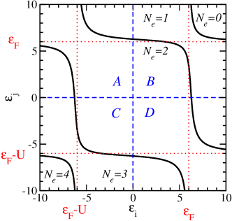
Figure 4: Phase diagram for an isolated pair $(i,j)$ of sites with site energies $\epsilon_{i}$ and $\epsilon_{j}$. The figure shows the number $N_{e}$ of electrons in the ground state, and is divided into four quadrants by the dashed blue lines. The quadrants are labelled A,…,D. For the 2-electron ground state, the most important regions are $\epsilon_{i}\sim\epsilon_{j}+U\sim{\varepsilon_{F}}$ (quadrant D) and $\epsilon_{i}+U\sim\epsilon_{j}\sim{\varepsilon_{F}}$ (quadrant A), which correspond to the LHO on one site and the UHO on the other being nearly degenerate with ${\varepsilon_{F}}$. For the 1-electron and 3-electron ground states, the most important regions of the phase diagram are $\epsilon_{i}\sim\epsilon_{j}\sim{\varepsilon_{F}}$ (quadrant B) and $\epsilon_{i}\sim\epsilon_{j}\sim{\varepsilon_{F}}-U$ (quadrant C) respectively.

Here, we calculate the derivative $\partial\Lambda^{\prime\prime}_{\mathrm{LHO}}(E)$ for an ensemble of pairs $(i,j)$ of isolated sites with random energies. The Green’s function for site $j$ with site $i$ removed is the atomic Green’s function

$$G^{i\kern-2.10002pt/}_{jj}(\omega) = \frac{h_{j{\overline{\sigma}}}}{\omega-\epsilon_{j}}+\frac{n_{j{\overline{\sigma}}}}{\omega-\epsilon_{j}-U},$$ (36)

$$= \frac{\omega-\epsilon_{j}-Uh_{j{\overline{\sigma}}}}{(\omega-\epsilon_{j})(\omega-\epsilon_{j}-U)},$$ (37)

where ${\overline{\sigma}}=-\sigma$, $h_{j{\overline{\sigma}}}=1-n_{j{\overline{\sigma}}}$, and where we suppress the spin index on $G$ in the nonmangnetic state. Using Eq. (37),

$$\Lambda^{\prime\prime}_{\epsilon_{i}}(\omega) = \frac{t^{2}U^{4}}{\Delta}\int_{-\Delta/2}^{\Delta/2}d\epsilon_{j}\frac{p_{ij}^{2}}{(\omega-\epsilon_{i}-Uh_{i{\overline{\sigma}}})^{2}(\omega-\epsilon_{j}-Uh_{j{\overline{\sigma}}})(\omega-\epsilon_{j})(\omega-\epsilon_{j}-U)},$$ (38)

and

$$\left.\frac{\partial\Lambda_{\epsilon_{i}}^{\prime\prime}(\omega)}{\partial\epsilon_{i}}\right|_{\omega=\epsilon_{i}} = \frac{t^{2}U^{2}}{\Delta}\int_{-\Delta/2}^{\Delta/2}d\epsilon_{j}\left[\partial_{\epsilon_{i}}p_{ij}^{2}-\frac{2p_{ij}^{2}(1+U\partial_{\epsilon_{i}}h_{i{\overline{\sigma}}})}{Uh_{i{\overline{\sigma}}}}-\frac{p_{ij}^{2}U\partial_{\epsilon_{i}}h_{j{\overline{\sigma}}}}{\epsilon_{j}+Uh_{j{\overline{\sigma}}}-\epsilon_{i}}\right]$$ (39)

$$\times\frac{-1}{h_{i{\overline{\sigma}}}^{2}(\epsilon_{j}+Uh_{j{\overline{\sigma}}}-\epsilon_{i})(\epsilon_{j}-\epsilon_{i})(\epsilon_{j}+U-\epsilon_{i})}$$

As discussed in the main text, the term in the square brackets proportional to $p_{ij}^{2}/Uh_{i{\overline{\sigma}}}$ is a factor $t/U$ smaller than the other terms, and is discarded.

Each pair of sites in the ensemble may have anywhere from 0 to 4 electrons, depending on $\epsilon_{i}$ and $\epsilon_{j}$, and in order to evaluate the integral in Eq. (39), we need to keep track of the different states. Figure 4 shows that there are four different possible ground states when $\epsilon_{i}$ is fixed near ${\varepsilon_{F}}$, having a total of $0$,$1$, $2$, or $3$ electrons shared between $i$ and $j$.

The 0-electron ground state does not contribute to $\partial\Lambda_{\mathrm{LHO}}(E)$ because $p_{ij}=0$. The 3-electron case also does not make a substantial contribution, in this case because the derivatives $\partial_{\epsilon_{i}}h_{i{\overline{\sigma}}}$, $\partial_{\epsilon_{i}}h_{j{\overline{\sigma}}}$, and $\partial_{\epsilon_{i}}p_{ij}$ are of order $t^{2}/U$. This follows because, in region D of the phase diagram (Fig. 4), the ground state wavefunction has the form

$$|3e\rangle\approx|\sigma 2\rangle-\frac{t}{\epsilon_{i}-\epsilon_{j}}|2\sigma\rangle,$$

where $|\sigma 2\rangle$ indicates that site $i$ has a single spin-$\sigma$ electron and that site $j$ is doubly occupied. Because $\epsilon_{i}-\epsilon_{j}\sim U$, the derivatives in Eq. (39) are of order $t/U^{2}$.

The remaining contributions to Eq. (39) are from the 1-electron and 2-electron ground states. It turns out that $p_{ij}^{2}$ is an order of magnitude smaller in the 1-electron case, where $\langle\hat{S}_{i+}\hat{S}_{j-}\rangle=0$, than in the 2-electron case, and so we focus our attention on the latter.

For $\epsilon_{i}\sim{\varepsilon_{F}}$, the most important contributions to the ZBA for the 2-electron case come from quadrant D of the phase diagram in Fig. 4. In this quadrant, there are two important configurations: the singlet $|s\rangle=(|\uparrow\downarrow\rangle-|\downarrow\uparrow\rangle)/\sqrt{2}$, and the double-occupancy state $|02\rangle$ which has both electrons on site $j$. These states have nearly the same energy, so we use degenerate perturbation theory. We project the AHM onto $|s\rangle$ and $|02\rangle$ to get the Hamiltonian matrix,

$$H_{2e}=\left[\begin{array}[]{cc}\epsilon_{i}+\epsilon_{j}&-\sqrt{2}t\\ -\sqrt{2}t&2\epsilon_{j}+U\end{array}\right]$$ (40)

from which follows the ground state wavefunction, $|2e\rangle=\alpha|s\rangle+\sqrt{1-\alpha^{2}}|02\rangle$, with

$$\alpha^{2}=\frac{1}{2}\left[1+\frac{y}{\sqrt{y^{2}+2t^{2}}}\right],$$ (41)

where $y=(\epsilon_{j}+U-\epsilon_{i})/2$. We can write the expectation values in Eq. (39) in terms of $\alpha^{2}$:

$$h_{i{\overline{\sigma}}} = 1-\frac{\alpha^{2}}{2},\quad h_{j{\overline{\sigma}}}=\frac{\alpha^{2}}{2},$$ (42)

$$p_{ij} = -\alpha^{2}\left(1-\frac{\alpha^{2}}{4}\right)\approx-\alpha^{2}$$ (43)

It simplifies our calculations significantly that the derivatives in Eq. (39) all reduce to derivatives of $\alpha^{2}$. We use $\partial_{\epsilon_{i}}=-\frac{1}{2}\partial_{y}$ and substitute $d\epsilon_{j}\rightarrow 2dy$ to obtain

$$\left.\frac{\partial\Lambda_{\epsilon_{i}}^{\prime\prime}(\omega)}{\partial\epsilon_{i}}\right|_{\omega=\epsilon_{i}}=\frac{t^{2}}{\Delta}\int_{y_{0}}^{y_{1}}\frac{dy}{y}\alpha^{2}(\partial_{y}\alpha^{2})\frac{1+\frac{\alpha^{2}}{4}}{1-\frac{\alpha^{2}}{2}}.$$ (44)

We need the principal part of the integral for $\partial\Lambda^{\prime\prime}_{\mathrm{LHO}}(E)$. In deriving this expression, we have neglected terms of order $t/U$.

The integration limits are given by the range of $y$ over which the ground state has two electrons. It can be shown that the 2-electron state is stable in region D of Fig. 4 forChen and Atkinson (2010)

$$\tilde{\epsilon}_{i}(\tilde{\epsilon}_{j}+U)<2t^{2},$$ (45)

where $\tilde{\epsilon}_{i,j}=\epsilon_{i,j}-{\varepsilon_{F}}$. The boundaries of the 2-electron phase in this region are shown as thick black lines in the figure. Setting $\epsilon_{i}=E$, we obtain the integration limits

$$y_{0} = \frac{t^{2}}{\tilde{E}}-\frac{\tilde{E}}{2},\qquad y_{1}=\infty,\qquad(\tilde{E}<0)$$ (46)

$$y_{0} = -\infty,\qquad y_{1}=\frac{t^{2}}{\tilde{E}}-\frac{\tilde{E}}{2},\qquad(\tilde{E}>0),$$ (47)

where $\tilde{E}=E-{\varepsilon_{F}}$. The integration limits at $\pm\infty$ come from the boundaries of region D, which are taken to be far from ${\varepsilon_{F}}$ and ${\varepsilon_{F}}-U$. This assumption does not change our results significantly because the integrand in Eq. (44) is peaked near $y=0$, because of the factor

$$\partial_{y}\alpha^{2}=\frac{t^{2}}{(y^{2}+2t^{2})^{3/2}}.$$

We, for the same reason, can expand

$$\left(1-\frac{\alpha^{2}}{2}\right)^{-4} = \left(\frac{4}{3}\right)^{4}\left(1-\frac{y}{3\sqrt{y^{2}+2t^{2}}}\right)^{-4}$$

$$\approx \left(\frac{4}{3}\right)^{4}\Bigg{[}1+\frac{4y}{3\sqrt{y^{2}+2t^{2}}}+\frac{10y^{2}}{9(y^{2}+2t^{2})}$$

$$+\ldots\Bigg{]}$$

and

$$1+\frac{\alpha^{2}}{4} = \frac{9}{8}+\frac{y}{8\sqrt{y^{2}+2t^{2}}}\approx\frac{9}{8}$$

to obtain

$$\partial\Lambda_{\mathrm{LHO}}^{\prime\prime}(E) = \left.\mbox{Re }\frac{\partial\Lambda_{\epsilon_{i}}^{\prime\prime}(\omega)}{\partial\epsilon_{i}}\right|_{\omega=\epsilon_{i}=E}$$

$$= \frac{4\sqrt{2}t}{9\Delta}\left[F_{1}\left(\frac{y}{\sqrt{2}t}\right)+\frac{7}{6}F_{2}\left(\frac{y}{\sqrt{2}t}\right)\right.$$

$$\left.-\frac{22}{27}F_{3}\left(\frac{y}{\sqrt{2}t}\right)+\frac{25}{54}F_{4}\left(\frac{y}{\sqrt{2}t}\right)\ldots\right]_{y_{0}}^{y_{1}},$$

where $F_{n}(x)=n\int dx\,{x^{n-2}}/{(1+x^{2})^{1+n/2}}$. The functions $F_{n}(x)$ are odd (even) when $n$ is even (odd). Because the limits $y_{0}$ and $y_{1}$ are odd in $\tilde{E}$, $F_{2}(x)$ and $F_{4}(x)$ actually make a contribution to $\partial\Lambda_{\mathrm{LHO}}(E)$ that is even in $\tilde{E}$. Using the symmetry of Eq. (17), it follows that

$$\partial\Lambda_{\mathrm{LHO}}^{\prime\prime}(E)+\partial\Lambda_{\mathrm{UHO}}^{\prime\prime}(E) = \frac{28\sqrt{2}t}{27\Delta}\left[F_{2}\left(\frac{y}{\sqrt{2}t}\right)\right.$$

$$\left.+\frac{25}{63}F_{4}\left(\frac{y}{\sqrt{2}t}\right)\right]_{y_{0}}^{y_{1}}$$

Explicitly,

$$F_{2}(x) = \frac{x}{x^{2}+1}+\tan^{-1}(x).$$ (50)

$$F_{4}(x) = \frac{1}{2}F_{2}(x)-\frac{x}{(1+x^{2})^{2}}$$ (51)

Appendix D Symmetries of $\partial\Lambda_{\mathrm{LHO}}(E)$ and $\partial\Lambda_{\mathrm{UHO}}(E)$

In this appendix, we prove the relation $\partial\Lambda_{\mathrm{UHO}}(E)=\partial\Lambda_{\mathrm{LHO}}(-E)$ (for convenience, we take ${\varepsilon_{F}}=0$ in this section). This result is based on the symmetries of the single-site Green’s function, Eq. (36), and the self-energy Eq. (14).

The proof proceeds as follows: $\partial\Lambda_{\mathrm{LHO}}(E)$ has contributions from 2-electron states in region D of Fig. 4 and 1-electron states in region B; $\partial\Lambda_{\mathrm{UHO}}(E)$ has contributions from 2-electron states in region A of Fig. 4 and 3-electron states in region C. We show that there is a correspondence between regions A and D, and between regions B and C, with the result that $\partial_{\epsilon}\Lambda_{\epsilon}(E)|_{\epsilon=E}$ in B (or D) is equal to $\partial_{\epsilon}\Lambda_{\epsilon}(-E)|_{\epsilon=E-U}$ in C (or A).

Suppressing subscripts, we write $\partial_{\epsilon}\Lambda_{\epsilon}(E)$, with $\Lambda_{\epsilon}(E)$ given by Eq. (16), as

$$\partial\Lambda=2\langle(-t+\Sigma)(\partial\Sigma)G\rangle+\langle(-t+\Sigma)^{2}\partial G\rangle.$$ (52)

Now consider a pair of sites with $\epsilon_{i}$ and $\epsilon_{j}$ belonging to region D, and a corresponding pair of sites with $\epsilon_{i}^{\prime}=\epsilon_{i}-U$, $\epsilon_{j}^{\prime}=\epsilon_{j}+U$ belonging to region A. For region D, the wavefunction is $|2e\rangle=\alpha_{y}|s\rangle+\sqrt{1-\alpha_{y}^{2}}|02\rangle$ with $y=(\epsilon_{j}+U-\epsilon_{i})/2$, while for region A, $|2e\rangle^{\prime}=\alpha_{y}|s\rangle+\sqrt{1-\alpha_{y}^{2}}|20\rangle$ with $y=(\epsilon_{i}+U-\epsilon_{j})/2$, where $\alpha_{y}$ is the same in both cases. Because of this symmetry, $h_{j{\overline{\sigma}}}^{\prime}=n_{j{\overline{\sigma}}}$ and $n_{j{\overline{\sigma}}}^{\prime}=h_{j{\overline{\sigma}}}$. It follows immediately that the local Green’s function Eq. (36) satisfies

$$G^{\prime}_{\epsilon_{i}+U=E}=-G_{\epsilon_{i}=E},\quad\partial G^{\prime}_{\epsilon_{i}+U=E}=\partial G_{\epsilon_{i}=E}$$ (53)

where $G^{\prime}$ is the Green’s function for primed site energies, and $G$ is for unprimed site energies. It also follows that $\Sigma_{ij}(E)\rightarrow\Sigma(y)$ for regions A and D, with $\Sigma(y)$ the same even function of $y$ in both cases, but with $y$ specific to each region, as above. Thus

$$\Sigma^{\prime}_{\epsilon_{i}=E-U}=\Sigma_{\epsilon_{i}=E},\quad\partial\Sigma^{\prime}_{\epsilon_{i}=E-U}=-\partial\Sigma_{\epsilon_{i}=E}.$$ (54)

Equations (53) and (54) suggest that $\partial\Lambda$ is even under $(\epsilon_{i},\epsilon_{j})\rightarrow(\epsilon_{i}^{\prime},\epsilon_{j}^{\prime})$; however, an additional negative sign arises from averaging over $j$. For $\epsilon_{i}$,

$$\int d\epsilon_{j}\ldots\rightarrow\int_{y_{0}}^{y_{1}}2dy\ldots,$$

while for $\epsilon_{i}^{\prime}$

$$\int d\epsilon_{j}^{\prime}\ldots\rightarrow\int_{-y_{1}}^{-y_{0}}2dy\ldots$$

Because of the inverted integration limits, we obtain (considering only contributions from regions A and D),

$$\partial_{\epsilon}\Lambda_{\epsilon}(E)|_{\epsilon=E}=\partial_{\epsilon}\Lambda_{\epsilon}(-E)|_{\epsilon=E-U}.$$ (55)

An identical result is found if we consider primed and unprimed site energies belonging to regions B and C respectively, which proves

$$\partial\Lambda_{\mathrm{LHO}}(E)=\partial\Lambda_{\mathrm{UHO}}(-E).$$ (56)

References

- Imada et al. (1998) M. Imada, A. Fujimori, and Y. Tokura, Rev. Mod. Phys. 70, 1039 (1998).
- Schneider et al. (2008) U. Schneider et al., Science 322, 1520 (2008).
- White et al. (2009) M. White, M. Pasienski, D. McKay, S. Q. Zhou, D. Ceperley, and B. DeMarco, Phys. Rev. Lett. 102, 055301 (2009).
- Zhou and Das Sarma (2010) Q. Zhou and S. Das Sarma, Phys. Rev. A 82, 041601 (2010).
- Tusch and Logan (1993) M. A. Tusch and D. E. Logan, Phys. Rev. B 48, 14843 (1993).
- Heidarian and Trivedi (2004) D. Heidarian and N. Trivedi, Phys. Rev. Lett. 93, 126401 (2004).
- Byczuk et al. (2005) K. Byczuk, W. Hofstetter, and D. Vollhardt, Phys. Rev. Lett. 94, 056404 (2005).
- Kotlyar and Das Sarma (2001) R. Kotlyar and S. Das Sarma, Phys. Rev. Lett. 86, 2388 (2001).
- Tanasković et al. (2003) D. Tanasković, V. Dobrosavljević, E. Abrahams, and G. Kotliar, Phys. Rev. Lett. 91, 066603 (2003).
- Paris et al. (2007) N. Paris, K. Bouadim, F. Hebert, G. G. Batrouni, and R. T. Scalettar, Phys. Rev. B 98, 046403 (pages 4) (2007).
- Chakraborty et al. (2007) P. B. Chakraborty, P. J. H. Denteneer, and R. T. Scalettar, Phys. Rev. B 75, 125117 (2007).
- Song et al. (2008) Y. Song, R. Wortis, and W. A. Atkinson, Phys. Rev. B 77, 054202 (2008).
- Henseler et al. (2008a) P. Henseler, J. Kroha, and B. Shapiro, Phys. Rev. B 77, 075101 (2008a).
- Henseler et al. (2008b) P. Henseler, J. Kroha, and B. Shapiro, Phys. Rev. B 78, 235116 (2008b).
- Andrade et al. (2009) E. C. Andrade, E. Miranda, and V. Dobrosavljevic, Physica B Cond. Mat. 404, 3167 (2009).
- Byczuk et al. (2009) K. Byczuk, W. Hofstetter, and D. Vollhardt, Phys. Rev. Lett. 102, 146403 (2009).
- Pezzoli and Becca (2010) M. E. Pezzoli and F. Becca, Phys. Rev. B 81, 075106 (2010).
- Semmler et al. (2010) D. Semmler, K. Byczuk, and W. Hofstetter, Phys. Rev. B 81, 115111 (2010).
- Lieb and Wu (1968) E. H. Lieb and F. Y. Wu, Phys. Rev. Lett. 20, 1445 (1968).
- Georges et al. (1996) A. Georges, G. Kotliar, W. Krauth, and M. J. Rozenberg, Rev. Mod. Phys. 68, 13 (1996).
- Dagotto (1994) E. Dagotto, Rev. Mod. Phys. 66, 763 (1994).
- Chiesa et al. (2008) S. Chiesa, P. B. Chakraborty, W. E. Pickett, and R. T. Scalettar, Phys. Rev. Lett. 101, 086401 (2008).
- Altshuler and Aronov (1985) B. L. Altshuler and A. G. Aronov, in Electron-electron interactions in disordered systems, edited by A. L. Efros and M. Pollak (North Holland, New York, 1985), vol. 10 of Modern Problems in Condensed Matter Sciences.
- Fazileh et al. (2006) F. Fazileh, R. J. Gooding, W. A. Atkinson, and D. C. Johnston, Phys. Rev. Lett. 96, 046410 (2006).
- Chen and Gooding (2009) X. Chen and R. J. Gooding, Phys. Rev. B 80, 115125 (2009).
- Shinaoka and Imada (2009a) H. Shinaoka and M. Imada, Phys. Rev. Lett. 102, 016404 (2009a).
- Shinaoka and Imada (2009b) H. Shinaoka and M. Imada, J. Phys. Soc. Jpn. 78, 094708 (2009b).
- Shinaoka and Imada (2010) H. Shinaoka and M. Imada, J. Phys. Soc. Jpn. 79, 094711 (2010).
- Ulmke et al. (1995) M. Ulmke, V. Janiš, and D. Vollhardt, Phys. Rev. B 51, 10411 (1995).
- Miranda and Dobrosavljević (2005) E. Miranda and V. Dobrosavljević, Rep. Prog. Phys. 68, 2337 (2005).
- Laad et al. (2001) M. S. Laad, L. Craco, and E. Müller-Hartmann, Phys. Rev. B 64, 195114 (2001).
- Balzer and Potthoff (2005) M. Balzer and M. Potthoff, Physica B 359-361, 768 (2005).
- Lombardo et al. (2006) P. Lombardo, R. Hayn, and G. I. Japaridze, Phys. Rev. B 74, 085116 (2006).
- Song et al. (2009) Y. Song, S. Bulut, R. Wortis, and W. A. Atkinson, J. Phys. Cond. Mat. 21, 385601 (13pp) (2009).
- Wortis and Atkinson (2010) R. Wortis and W. A. Atkinson, Phys. Rev. B 82, 073107 (2010).
- Chen and Atkinson (2010) H.-Y. Chen and W. A. Atkinson, Phys. Rev. B 82, 125108 (2010).
- (37) R. Wortis and W. A. Atkinson, http://arxiv.org/abs/1008.2245v1.
- Abrahams et al. (1981) E. Abrahams, P. W. Anderson, P. A. Lee, and T. V. Ramakrishnan, Phys. Rev. B 24, 6783 (1981).
- Golub and van Loan (1996) G. H. Golub and C. F. van Loan, Matrix Computations (Johns Hopkins, 1996), 3rd ed.
- (40) There is some subtlety in how is defined. In the noninteracting case, is completely independent of . However, in the intereacting case, the self-energies used in evaluating are the same as the self-energies of the full lattice except that nonlocal matrix elements are set to 0. This means that depends implicitly on through the self-energy.
- Odashima et al. (2005) S. Odashima, A. Avella, and F. Mancini, Phys. Rev. B 72, 205121 (2005).