A faithful linear-categorical action of the mapping class group of a surface with boundary

Abstract.

We show that the action of the mapping class group on bordered Floer homology in the second to extremal $\operatorname{spin}^{c}$-structure is faithful. This paper is designed partly as an introduction to the subject, and much of it should be readable without a background in Floer homology.

1. Introduction

Two long-standing, and apparently unrelated, questions in low-dimensional topology are whether the mapping class group of a surface is linear and whether the Jones polynomial detects the unknot. In 2010, Kronheimer-Mrowka gave an affirmative answer to a categorified version of the second question: they showed that Khovanov homology, a categorification of the Jones polynomial, does detect the unknot [KM11]. (Previously, Grigsby and Wehrli had shown that any nontrivially-colored Khovanov homology detects the unknot [GW10].) In this paper, we give an affirmative answer to a categorified version of the first question. That is, while we do not know if the mapping class group of a surface (with boundary) acts faithfully on a finite-dimensional linear space, we are able to give an explicit faithful action on a finitely-generated linear (in fact, triangulated) category. The decategorification of this action is the standard action of the mapping class group on $H_{1}$; see Theorem 4 in Section 5.

In more detail, the structure is as follows. To a surface $F$ with boundary and a marked point on each boundary component, we associate a finite-dimensional algebra $\mathcal{B}(F)$ over ${\mathbb{F}_{2}}=\mathbb{Z}/2$. (There is some choice in the definition of $\mathcal{B}(F)$; see Section 2.) To a mapping class $\phi\colon F\to F$, fixing the boundary, we associate a quasi-isomorphism class of finite-dimensional differential $\mathcal{B}(F)$-bimodules $\widehat{\mathit{CFDA}}(\phi)$. These have the property that

(1.1) $$\widehat{\mathit{CFDA}}(\psi\circ\phi)\simeq\widehat{\mathit{CFDA}}(\phi)\otimes_{\mathcal{B}(F)}\widehat{\mathit{CFDA}}(\psi).$$

Moreover,

(1.2) $$\widehat{\mathit{CFDA}}(\mathbb{I}) \simeq{}_{\mathcal{B}(F)}\mathcal{B}(F)_{\mathcal{B}(F)},$$

where ${}_{\mathcal{B}(F)}\mathcal{B}(F)_{\mathcal{B}(F)}$ denotes the algebra $\mathcal{B}(F)$ viewed as a bimodule over itself.

Let ${}_{\mathcal{B}(F)}\mathsf{Mod}$ denote the category of finitely-generated left $\mathcal{B}(F)$-modules. For each mapping class $\phi$ we have a functor $\Phi_{\phi}\colon{}_{\mathcal{B}(F)}\mathsf{Mod}\to{}_{\mathcal{B}(F)}\mathsf{Mod}$ given by $\Phi_{\phi}(\cdot)=\widehat{\mathit{CFDA}}(\phi)\otimes_{\mathcal{B}(F)}\cdot$. Equations (1.1) and (1.2) almost imply that this is an action; the main defect is that Equation (1.1) only gives homotopy equivalences, not isomorphisms (or equalities). To rectify this, we replace ${}_{\mathcal{B}(F)}\mathsf{Mod}$ with the associated derived category $\mathcal{D}^{b}({}_{\mathcal{B}(F)}\mathsf{Mod})$ of finitely-generated modules. (This is quite concrete: since finite-dimensional modules over our algebras admit finite-dimensional projective resolutions, $\mathcal{D}^{b}({}_{\mathcal{B}(F)}\mathsf{Mod})$ is just the homotopy category of finitely-generated projective modules over $\mathcal{B}(F)$.) Equations (1.1) and (1.2) then imply that tensoring with the modules $\widehat{\mathit{CFDA}}(\psi)$ gives an action of the mapping class group on $\mathcal{D}^{b}({}_{\mathcal{B}(F)}\mathsf{Mod})$. (There are some subtleties related to group actions on categories. See for example [LOT10a, Section 8] for a review of the relevant definitions.)

The bimodules $\widehat{\mathit{CFDA}}(\phi)$ carry geometric information. In particular, the rank of the homology of $\widehat{\mathit{CFDA}}(\phi)$ is given by a certain intersection number. This turns out to be enough to prove that

(1.3) $$\widehat{\mathit{CFDA}}(\phi)\not\simeq\widehat{\mathit{CFDA}}(\mathbb{I})\qquad\text{if }\phi\not\sim\mathbb{I}.$$

As a corollary, we have:

Theorem 1.

The action of the mapping class group $\mathit{MCG}_{0}(F)$ on $\mathcal{D}^{b}({}_{\mathcal{B}(F)}\mathsf{Mod})$ given by tensoring with the bimodules $\widehat{\mathit{CFDA}}(\phi)$ is faithful.

In fact, there are two different ways we can do this construction combinatorially. One leads to somewhat simpler algebras, but more complicated ($\mathcal{A}_{\infty}$) bimodules; the other leads to more complicated (differential) algebras but simpler (differential) bimodules. Although these two actions are equivalent in a certain sense—see Proposition 3.27, below—we will give both approaches.

Experts in bordered Floer theory are warned that throughout this paper we are working in the second to extremal $\operatorname{spin}^{c}$-structure. In the notation of [LOT08], the algebras $\mathcal{B}(F)$ (respectively $\mathcal{C}(F)$) in this paper are $\mathcal{A}(F,\allowbreak-g+1)$ (respectively $\mathcal{A}(F,\allowbreak g-1)$), where $g$ is the genus of $F$, and the bimodules $\widehat{\mathit{CFDA}}(\phi)$ are the corresponding summands of the bimodules $\widehat{\mathit{CFDA}}(\phi)$ from [LOT10a].

This paper has two main goals. The first goal is to prove faithfulness of the mapping class group action (Theorem 1). The proof of faithfulness itself is short, and the reader familiar with the bordered Floer package may wish to skip directly to Section 4 (perhaps after perusing some of the pictures earlier in the paper), where the proof is given. The second goal is to give a combinatorial description of this mapping class group action (in the second to extremal $\operatorname{spin}^{c}$-structure). This paper is partly intended as an introduction to the subject. So, we include a complete description of the relevant algebras and modules. The proof of faithfulness is also elementary, and both the modules and the faithfulness proof are closely related to familiar tools in mapping class group theory. We do not give self-contained proofs that the bimodules associated to mapping classes are well-defined, or that tensoring with them gives a well-defined action; these results draw on [LOT10a], which uses the theory of pseudoholomorphic curves. Since the first version of this paper was written, Kyler Siegel has given direct combinatorial proofs of these facts; see [Sie11].

In this paper, we treat mapping class groups of any surface with non-empty boundary. The case of actions of braid groups on triangulated categories (unlike the more general case) has received substantial attention in the literature. See in particular [KS02], and also [KT07] and the references contained therein. Another triangulated category on which the mapping class group acts is the Fukaya category of a surface; a theorem of Seidel [Sei02, Theorem 1], together with a folk conjecture relating the Hochschild homology of functors on the Fukaya category and Floer homology of symplectomorphisms, should imply this action is faithful for a closed surface. The argument in Section 4, which was inspired by [KS02], can be adapted to give a more direct proof of faithfulness of the action on the Fukaya category of a surface; this is presumably well-known in certain circles. In contrast with the Fukaya category, the triangulated categories constructed in this paper are purely algebraic, and have finiteness properties which are not apparent for the Fukaya category. There is, however, a direct relation between the constructions in this paper and a variant of the Fukaya category; see [Aur10].

This paper is structured as follows. In Section 2 we define the algebras $\mathcal{B}(F)$; these are more general than the algebras from [LOT08], since we allow $F$ to have more than one boundary component, but are special cases of definitions from [Zar09]. In Section 3 we define the bimodules. In Section 4 we prove faithfulness of the action. In Section 5 we discuss a sense in which these categories are finitely generated, and the decategorification of our action. We conclude, in Section 6, with some further questions.

1.1. Acknowledgements.

We thank T. Cochran, E. Grigsby and S. Harvey for helpful conversations, and C. Clarkson and K. Siegel for helpful comments on an earlier version of this paper. The proof of faithfulness is inspired by the argument in [KS02]. We also thank the Mathematical Sciences Research Institute and Columbia University for hosting us during this research. Finally, we thank the referee for many helpful comments.

2. The algebras

In the present section, we define two algebras associated to an arc diagram $\mathcal{Z}$, denoted $\mathcal{B}(\mathcal{Z})$ (Section 2.2) and $\mathcal{C}(\mathcal{Z})$ (Section 2.3). The second of these, $\mathcal{C}(\mathcal{Z})$, is equipped with a differential, while the first, $\mathcal{B}(\mathcal{Z})$, is not. These are both subalgebras of a more general algebra $\mathcal{A}(\mathcal{Z})$, which we introduce in Section 2.3. These algebras can be endowed with further structure (notably, a kind of grading), which we will not need here; see [LOT08].

Before defining the algebras, we recall a convenient way of representing surfaces.

2.1. Arc diagrams

Consider a connected, oriented surface $F$ of genus $g$ with $b>0$ boundary components $Z_{1},\dots,Z_{b}$, and suppose that each $Z_{i}$ is divided into two closed arcs, $S_{i}^{+}$ and $S_{i}^{-}$ (overlapping at their endpoints); write $S^{+}=\cup_{i}S_{i}^{+}$ and $S^{-}=\cup_{i}S_{i}^{-}$. Choose a collection of pairwise-disjoint, embedded paths $\alpha_{i}$ in $F$ with $\partial\alpha_{i}\subset S^{+}$ so that $F\setminus(\cup_{i}\alpha_{i})$ is a union of disks, and the boundary of each disk contains exactly one $S_{i}^{-}$. This implies that we have exactly $2(g+b-1)$ $\alpha$-curves. Place a basepoint $z_{i}$ in each $S_{i}^{-}$.

Let $\{a_{i},a^{\prime}_{i}\}=\partial\alpha_{i}$. We call

$$\mathcal{Z}=(\overbrace{(Z_{1},\dots,Z_{b})}^{Z},\overbrace{(\{a_{1},a^{\prime}_{1}\},\dots,\{a_{n},a^{\prime}_{n}\})}^{M},\overbrace{(z_{1},\dots,z_{b})}^{\mathbf{z}})$$

an arc diagram for $F$. Write ${\mathbf{a}}=\{a_{1},a^{\prime}_{1},\dots,a_{2(g+b-1)},a^{\prime}_{2(g+b-1)}\}$. Here, the $Z_{i}$ are viewed as oriented circles. For each $i$, the points $a_{i}$ and $a_{i}^{\prime}$ are called a matched pair.

From $\mathcal{Z}$ we can build a standard model surface as follows. Thicken the circles $Z_{i}$ in $Z$ to annuli $[0,1]\times Z_{i}$ and attach strips ($2$-dimensional $1$-handles) to each pair of points in $M$ in the outer boundaries $\{1\}\times Z_{i}$ of the annuli. Call the result $F^{\circ}(\mathcal{Z})$. The basepoint $z_{i}$ in $Z_{i}$ gives an arc $\gamma_{z_{i}}=[0,1]\times\{z_{i}\}\subset[0,1]\times Z_{i}$. Let $F(\mathcal{Z})$ denote the result of cutting $F^{\circ}(\mathcal{Z})$ along the $\gamma_{z_{i}}$. Let $S^{+}(\mathcal{Z})$ be the part of $\partial F(\mathcal{Z})$ coming from $\bigcup_{i}\{0\}\times Z_{i}$, together with the part corresponding to the $\gamma_{z_{i}}$, and let $S^{-}(\mathcal{Z})$ be the part of $\partial F(\mathcal{Z})$ coming from $\bigcup_{i}\{1\}\times Z_{i}$ (and the handles attached to it). See Figure 1.

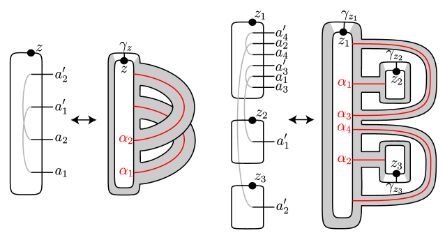
Figure 1. Arc diagrams and their associated surfaces. Left: an arc diagram specifying a once-punctured torus. Right: an arc diagram specifying the $3$-times punctured sphere. In each case, the subsurface $F(\mathcal{Z})\subset F^{\circ}(\mathcal{Z})$ is shaded.

The choice of the $\alpha_{i}$ identifies $F$ and $F(\mathcal{Z})$ canonically (up to isotopy).

Remark 2.1.

Let $\mathcal{Z}=(Z,M,\mathbf{z})$ be an arc diagram for $F$. By definition, each circle in $Z$ contains one point $z_{i}\in\mathbf{z}$. Moreover, performing surgery on $Z$ along the pairs of points in $M$ gives a collection of circles each of which also contains a single $z_{i}$. Conversely, any triple $(Z,M,\mathbf{z})$ satisfying this condition comes from a surface.

Remark 2.2.

We are considering a special case of Zarev’s definition of arc diagrams [Zar09]: he allows each $Z_{i}$ to be divided into $2n_{i}$ arcs for any $n_{i}\in\mathbb{N}$.

2.2. The algebra $\mathcal{B}(\mathcal{Z})$

The algebras of interest are associated to arc diagrams. The algebra $\mathcal{B}(\mathcal{Z})$ has a basis over ${\mathbb{F}_{2}}$ consisting of:

• One element $I_{i}$ for each pair of points $\{a_{i},a^{\prime}_{i}\}\in M$.

• One element $\rho$ for each nontrivial interval in each $Z_{i}\setminus\{z_{i}\}$ with endpoints in ${\mathbf{a}}$. We will call these elements chords. Given a chord $\rho$, let $\rho^{-}$ denote the initial point of $\rho$ (with respect to the orientation on $Z_{i}$), and let $\rho^{+}$ denote the terminal point of $\rho$.

The product on the algebra is given as follows:

• The $I_{i}$ are orthogonal idempotents, so $I_{i}^{2}=I_{i}$ and $I_{i}I_{j}=0$ if $i\neq j$.

• $I_{i}\rho=\rho$ if $\rho^{-}$ is $a_{i}$ or $a^{\prime}_{i}$; otherwise, $I_{i}\rho=0$. Similarly, $\rho I_{j}=\rho$ if $\rho^{+}$ is $a_{j}$ or $a^{\prime}_{j}$; otherwise, $\rho I_{j}=0$.

• For chords $\rho$ and $\sigma$, $\rho\sigma=0$ unless $\rho^{+}=\sigma^{-}$. If $\rho^{+}=\sigma^{-}$ then $\rho\sigma$ is the chord from $\rho^{-}$ to $\sigma^{+}$.

Example 2.3.

There is a unique arc diagram $\mathcal{Z}$ for the once-punctured torus, which is illustrated in Figure 1. The algebra $\mathcal{B}(\mathcal{Z})$ is $8$-dimensional, with basis

$$\{I_{1},I_{2},\rho_{1,2},\rho_{2,3},\rho_{3,4},\rho_{1,3},\rho_{2,4},\rho_{1,4}\}$$

and multiplication table

$$\begin{array}[]{l|@{\quad}llllllll}\hlx{v}\times&I_{1}&I_{2}&\rho_{1,2}&\rho_{2,3}&\rho_{3,4}&\rho_{1,3}&\rho_{2,4}&\rho_{1,4}\\ \hlx{hvv}I_{1}&I_{1}&0&\rho_{1,2}&0&\rho_{3,4}&\rho_{1,3}&0&\rho_{1,4}\\ I_{2}&0&I_{2}&0&\rho_{2,3}&0&0&\rho_{2,4}&0\\ \rho_{1,2}&0&\rho_{1,2}&0&\rho_{1,3}&0&0&\rho_{1,4}&0\\ \rho_{2,3}&\rho_{2,3}&0&0&0&\rho_{2,4}&0&0&0\\ \rho_{3,4}&0&\rho_{3,4}&0&0&0&0&0&0\\ \rho_{1,3}&\rho_{1,3}&0&0&0&\rho_{1,4}&0&0&0\\ \rho_{2,4}&0&\rho_{2,4}&0&0&0&0&0&0\\ \rho_{1,4}&0&\rho_{1,4}&0&0&0&0&0&0\\ \hlx{v}\end{array}$$

(When reading this table, the third entry in the top row, e.g., means that $I_{1}\rho_{1,2}=\rho_{1,2}$.)

We can encode this algebra more succinctly as

Example 2.4.

Let $F$ be a genus $g$ surface with one boundary component. One arc diagram for $F$ is obtained as follows. Label $4g+1$ points on a circle $Z$, in order, by

$$z,a_{1},\dots,a_{2g},a^{\prime}_{1},\dots,a^{\prime}_{2g}.$$

The algebra $\mathcal{B}(\mathcal{Z})$ associated to this arc diagram $\mathcal{Z}$ has idempotents $I_{1},\dots,I_{2g}$. For convenience, define $I_{i+2g}=I_{i}$. Then $\mathcal{B}(\mathcal{Z})$ is generated over ${\mathbb{F}_{2}}$ by $I_{1},\dots,I_{2g}$ and elements $\rho_{i,j}$ for $1\leq i<j\leq 4g$, with the relations:

$$I_{i}\rho_{i,j}I_{j} =\rho_{i,j},$$

$$I_{i}\rho_{j,k}=\rho_{j,k}I_{i} =0\qquad\text{(in cases not covered above),}$$

$$\rho_{i,j}\rho_{k,l} =\begin{cases}\rho_{i,l}&\text{if }j=k,\\ 0&\text{otherwise.}\end{cases}$$

Graphically, this is:

$$\vbox{\hbox{$\leavevmode\hbox to293.5pt{\vbox to67.98pt{\text{[drawing]}}}$}}\bigg{/}\left(\begin{array}[]{l}\rho_{i,i+1}\rho_{2g+i,2g+i+1}=0\\ \rho_{2g+i,2g+i+1}\rho_{i,i+1}=0\end{array}\right). I_{1} I_{2} \cdots\! I_{2g} \rho_{1,2} \rho_{2g+1,2g+2} \rho_{2,3} \rho_{2g+2,2g+3} \rho_{2g-1,2g} \rho_{4g-1,4g} \rho_{2g,2g+1} I_{1} I_{2} \cdots\! I_{2g} \rho_{1,2} \rho_{2g+1,2g+2} \rho_{2,3} \rho_{2g+2,2g+3} \rho_{2g-1,2g} \rho_{4g-1,4g} \rho_{2g,2g+1}$$

See also [AGW11], where this algebra is related to the algebras in [KS02].

Example 2.5.

There is an arc diagram for the complement of $k>0$ disks in $S^{2}$ that generalizes Figure 1 (right). On one circle $Z_{1}$, label $3k-2$ points by

$$z_{1},a_{1},b_{1},a^{\prime}_{1},a_{2},b_{2},a^{\prime}_{2},\dots,a_{k-1},b_{k-1},a^{\prime}_{k-1}.$$

On each remaining $Z_{i}$ ($i=2,\dots,k$) place two points $z_{i}$ and $b^{\prime}_{i}$. This represents a relabeling from Figure 1; see Figure 2.

Figure 2. Arc diagram for a thrice-punctured sphere. This is a relabeling of the diagram from Figure 1 (right).

The associated algebra has idempotents $I_{i}$ ($i=1,\dots,k-1$) corresponding to the $\{a_{i},a^{\prime}_{i}\}$ and $J_{i}$ ($i=1,\dots,k-1$) corresponding to the $\{b_{i},b^{\prime}_{i}\}$. The algebra is given by

$$\vbox{\hbox{$\leavevmode\hbox to280.95pt{\vbox to88.24pt{\text{[drawing]}}}$}}\!\!\!\bigg{/}\biggl{(}\begin{array}[]{l}\rho_{b_{i},a^{\prime}_{i}}\rho_{a_{i},b_{i}}=0\\ \rho_{a^{\prime}_{i},a_{i+1}}\rho_{a^{\prime}_{i+1},a_{i+2}}=0\end{array}\biggr{)}. I_{1} J_{1} I_{2} J_{2} \cdots\! I_{k-1} J_{k-1} \rho_{a_{1},b_{1}} \rho_{b_{1},a^{\prime}_{1}} \rho_{a^{\prime}_{1},a_{2}} \rho_{a_{2},b_{2}} \rho_{b_{2},a^{\prime}_{2}} \rho_{a^{\prime}_{2},a_{3}} \rho_{a^{\prime}_{k-2},a_{k-1}} \rho_{a_{k-1},b_{k-1}} \rho_{b_{k-1},a^{\prime}_{k-1}} I_{1} J_{1} I_{2} J_{2} \cdots\! I_{k-1} J_{k-1} \rho_{a_{1},b_{1}} \rho_{b_{1},a^{\prime}_{1}} \rho_{a^{\prime}_{1},a_{2}} \rho_{a_{2},b_{2}} \rho_{b_{2},a^{\prime}_{2}} \rho_{a^{\prime}_{2},a_{3}} \rho_{a^{\prime}_{k-2},a_{k-1}} \rho_{a_{k-1},b_{k-1}} \rho_{b_{k-1},a^{\prime}_{k-1}}$$

The following observation will be useful later:

Lemma 2.6.

Let $\mathcal{Z}$ be an arc diagram and $-\mathcal{Z}$ the arc diagram obtained by reversing the orientation of each circle $Z_{i}$ in $\mathcal{Z}$. Then $\mathcal{B}(-\mathcal{Z})$ is the opposite algebra to $\mathcal{B}(\mathcal{Z})$.

Proof.

This is immediate from the definitions. ∎

2.3. The algebra $\mathcal{C}(\mathcal{Z})$

Next we turn to the algebra $\mathcal{C}(\mathcal{Z})$. As mentioned in the introduction, we give two different constructions, with $\mathcal{B}(\mathcal{Z})$ and with $\mathcal{C}(\mathcal{Z})$; either one gives a faithful action. As such, this section may be skipped at first reading.

Let $\mathcal{Z}$ be an arc diagram for a surface of genus $g$ with $b$ boundary components. Let $n=2(g+b-1)$, so in particular the set ${\mathbf{a}}$ of marked points has $2n$ elements.

Consider $[0,1]\times(Z\setminus\mathbf{z})$. For each $i$ we can identify $[0,1]\times(Z_{i}\setminus z_{i})$ with $[0,1]\times(-1,1)$. The points ${\mathbf{a}}\cap Z_{i}$ give points $\{0\}\times{\mathbf{a}}_{i}\subset\{0\}\times(-1,1)$ and $\{1\}\times{\mathbf{a}}_{i}\subset\{1\}\times(-1,1)$.

A strand diagram for $\mathcal{Z}$ is a map $s\colon\coprod_{i=1}^{k}[0,1]\to[0,1]\times(Z\setminus\mathbf{z})$ (for some $k$), the components of which we call strands, considered up to reordering the strands, so that:

• $s$ maps $\coprod_{i=1}^{k}\{0\}$ to $\{0\}\times{\mathbf{a}}\subset\{0\}\times Z$ and $\coprod_{i=1}^{k}\{1\}$ to $\{1\}\times{\mathbf{a}}\subset\{1\}\times Z$.

• On each component of the source, $s$ is linear and has non-negative slope.

• The map $s|_{\coprod_{i=1}^{k}\{0\}}$ is injective, as is the map $s|_{\coprod_{i=1}^{k}\{1\}}$.

• For each matched pair $\{a_{i},a^{\prime}_{i}\}$, if there is a slope-zero strand (component of $s$) starting at $(0,a_{i})$ (respectively $(0,a^{\prime}_{i})$) then there is a slope-zero strand starting at $(0,a^{\prime}_{i})$ (respectively $(0,a_{i})$).

• For each matched pair $\{a_{i},a^{\prime}_{i}\}$, if there is a positive-slope strand starting at $(0,a_{i})$ (respectively $(0,a^{\prime}_{i})$) then there is no strand starting at $(0,a^{\prime}_{i})$ (respectively $(0,a_{i})$).

• For each matched pair $\{a_{i},a^{\prime}_{i}\}$, if there is a positive-slope strand ending at $(1,a_{i})$ (respectively $(1,a^{\prime}_{i})$) then there is no strand ending at $(1,a^{\prime}_{i})$ (respectively $(1,a_{i})$).

Consider the ${\mathbb{F}_{2}}$-vector space $\mathcal{A}(\mathcal{Z})$ generated by the strand diagrams. Define a product on this vector space as follows. Given $s,t\in\mathcal{A}(\mathcal{Z})$, the product of $s$ and $t$ is zero if

• there is a positive-slope strand in $s$ whose terminal endpoint is not the initial endpoint of a strand in $t$;

• there is a positive-slope strand in $t$ whose initial endpoint is not the terminal endpoint of a strand in $s$;

• there is a pair of slope-zero strands in $s$ neither of whose terminal endpoints is the initial endpoint of a strand in $t$;

• there is a pair of slope-zero strands in $t$ neither of whose initial endpoints is the terminal endpoint of a strand in $s$; or

• concatenating $s$ and $t$ end-to-end, there is a pair of piecewise-linear paths intersecting in two points (or equivalently, intersecting non-minimally).

See Figure 3. In other cases, $s\cdot t$ is gotten by concatenating $s$ and $t$, deleting any horizontal strands from $s$ (respectively $t$) which do not match with strands in $t$ (respectively $s$), and pulling the resulting piecewise-linear paths straight (fixing their endpoints). See Figure 4.

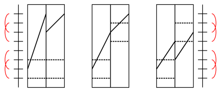
Figure 3. Examples of $0$ products in $\mathcal{A}$. The picture on the left illustrates the first two reasons the product can be zero, the picture in the middle illustrates the third and fourth reasons, and the picture on the right illustrates the last reason. When drawing elements of $\mathcal{A}$, we typically draw horizontal strands as dashed. This figure also appears in [LOT10b].

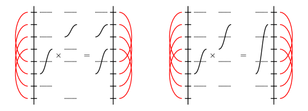
Figure 4. Two nontrivial products. Both take place in $\mathcal{C}(\mathcal{Z})\subset\mathcal{A}(\mathcal{Z})$ for $\mathcal{Z}$ the arc diagram from Example 2.4. We have drawn the strands slightly curved, rather than straight, for artistic effect.

Define a differential on $\mathcal{A}(\mathcal{Z})$ as follows. Given a strand diagram $s$ and a pair of intersecting strands $a,b$ in $s$, there is a unique (up to isotopy) way to resolve the intersection between $a$ and $b$ so that each resulting strand connects $\{0\}\times Z$ to $\{1\}\times Z$. If this resolution creates double-crossings between any pair of strands, let $s^{\prime}_{a,b}=0$; otherwise, let $s^{\prime}_{a,b}$ be the result of pulling straight the strands in the resolution and, if $a$ (respectively $b$) had slope $0$, deleting the slope-zero strand at $a^{\prime}$ (respectively $b^{\prime}$). Now, define

$$\partial(s)=\sum_{a,b\text{ intersect}}s^{\prime}_{a,b}.$$

See Figure 5.

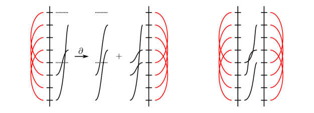
Figure 5. A differential. Left: an algebra element in $\mathcal{C}(\mathcal{Z})$, for $\mathcal{Z}$ the arc diagram from Example 2.4, and its differential. Right: a term which does not appear in the differential, because of a double-crossing. Again, we have drawn the strands slightly curved.

It is easy to verify that this multiplication and differential make $\mathcal{A}(\mathcal{Z})$ into a differential algebra. The minimal idempotents for $\mathcal{C}(\mathcal{Z})$ are strand diagrams in which all of the strands have slope $0$, and so correspond to subsets of the matched pairs in $M$.

Remark 2.7.

It is easy to turn this geometric definition of $\mathcal{A}(\mathcal{Z})$ into a combinatorial one; see, for instance, [LOT08].

The weight of a strand diagram $s$ is the number of positive-slope strands in $s$ plus half the number of slope-zero strands in $s$. Let $\mathcal{A}(\mathcal{Z},k)$ be the subalgebra of $\mathcal{A}(\mathcal{Z})$ generated by strand diagrams of weight $k+n/2$. Then

$$\mathcal{A}(\mathcal{Z})=\bigoplus_{k=-n/2}^{n/2}\mathcal{A}(\mathcal{Z},k).$$

Lemma 2.8.

The algebra $\mathcal{B}(\mathcal{Z})$ is $\mathcal{A}(\mathcal{Z},-n/2+1).$

Proof.

This is immediate from the definitions. ∎

Remark 2.9.

The algebra $\mathcal{A}(\mathcal{Z},-n/2)$ is ${\mathbb{F}_{2}}$ (generated by the empty strand diagram). The algebra $\mathcal{A}(\mathcal{Z},n/2)$ is quasi-isomorphic to ${\mathbb{F}_{2}}$; compare Remark 2.14.

Definition 2.10.

Let $\mathcal{C}(\mathcal{Z})=\mathcal{A}(\mathcal{Z},n/2-1).$

In particular the algebra $\mathcal{C}(\mathcal{Z})$ has $n$ minimal idempotents, corresponding to the choices of $n-1$ of the $n$ matched pairs in $M$.

Given a chord $\rho$ in $\mathcal{Z}$, let $c(\rho)\in\mathcal{C}(\mathcal{Z})$ be the sum of all ways of adding horizontal strands to $\rho$ to get an element of $\mathcal{C}(\mathcal{Z})$. (There are either $n-1$ such ways if the endpoints of $\rho$ are matched, or a single such choice if the endpoints of $\rho$ are not matched.)

Example 2.11.

For $\mathcal{Z}$ the unique pointed matched circle for the torus, $\mathcal{C}(\mathcal{Z})\cong\mathcal{B}(\mathcal{Z})$, which is described explicitly in Example 2.3.

Example 2.12.

Let $\mathcal{Z}$ be the arc diagram from Example 2.5 for the complement of $k$ disks in $S^{2}$. The algebra $\mathcal{C}(\mathcal{Z})$ is quite large. However, as we will see, $\mathcal{C}(\mathcal{Z})$ is formal; in fact, there is a map of algebras $f\colon\mathcal{C}(\mathcal{Z})\to H_{*}(\mathcal{C}(\mathcal{Z}))$ such that $f$ takes cycles to their homology classes. This means that in practice we can work with $H_{*}(\mathcal{C}(\mathcal{Z}))$, which we describe explicitly below, instead of $\mathcal{C}(\mathcal{Z})$.

To compute $H_{*}(\mathcal{C}(\mathcal{Z}))$ (and see that $\mathcal{C}(\mathcal{Z})$ is formal), we use a little more terminology. Given a strand diagram $s\in\mathcal{C}(\mathcal{Z})$, the support $\operatorname{supp}(s)$ of $s$ is the element of $H_{1}(Z,{\mathbf{a}})$ gotten by projecting $s$ to $Z$ and viewing the result as a $1$-chain.

As a first step towards understanding $H_{*}(\mathcal{C}(\mathcal{Z}))$, let $M\subset\mathcal{C}(\mathcal{Z})$ be the ${\mathbb{F}_{2}}$-subspace generated by strand diagrams $s$ such that $\operatorname{supp}(s)$ has multiplicity $>1$ somewhere. Then $M$ is a differential ideal in $H_{*}(\mathcal{C}(\mathcal{Z}))$. Further, $M$ is contractible, as in any arc diagram—see [LOT10a, Theorem 9]. So, it suffices to show that $\mathcal{C}^{\prime}(\mathcal{Z})=\mathcal{C}(\mathcal{Z})/M$ is formal.

Let $D$ be the ${\mathbb{F}_{2}}$-subspace of $\mathcal{C}^{\prime}(\mathcal{Z})$ generated by all strand diagrams $s\in\mathcal{C}^{\prime}(\mathcal{Z})$ such that the interior of the $\operatorname{supp}(s)$ contains some point $b_{i}\in{\mathbf{a}}$ which is occupied in the initial (and hence also in the terminal) idempotent. Then $D$ is a differential ideal in $\mathcal{C}(\mathcal{Z})$. We claim that $D$ is contractible. To see this, consider a strand diagram $s\in D$. Such strand diagrams have one of two forms: either $s$ has some strand starting at a point $b_{i}$ (and hence also a strand ending at $b_{i}$) or it does not. The generators of the two types cancel in pairs: each generator of the first type occurs in the differential of a unique generator of the second type.

Thus, we have reduced to considering $\mathcal{C}^{\prime\prime}(\mathcal{Z})=\mathcal{C}^{\prime}(\mathcal{Z})/D$. It is now easy to see that the homology of $\mathcal{C}^{\prime\prime}(\mathcal{Z})$ is given by:

$$\vbox{\hbox{$\leavevmode\hbox to280.95pt{\vbox to88.24pt{\text{[drawing]}}}$}}\!\!\!\Bigg{/}\Biggl{(}\begin{array}[]{l}\rho_{a_{i}^{\prime},a_{i+1}}\rho_{b_{i},a^{\prime}_{i}}=0\\ \rho_{a_{i},b_{i}}\rho_{a^{\prime}_{i-1},a_{i}}=0\\ \rho_{b_{i},a^{\prime}_{i}}\rho_{a_{i},b_{i}}=0\end{array}\Biggr{)}. I_{1} J_{1} I_{2} J_{2} \cdots\! I_{k-1} J_{k-1} \rho_{a_{1},b_{1}} \rho_{b_{1},a^{\prime}_{1}} \rho_{a^{\prime}_{1},a_{2}} \rho_{a_{2},b_{2}} \rho_{b_{2},a^{\prime}_{2}} \rho_{a^{\prime}_{2},a_{3}} \rho_{a^{\prime}_{k-2},a_{k-1}} \rho_{a_{k-1},b_{k-1}} \rho_{b_{k-1},a^{\prime}_{k-1}} I_{1} J_{1} I_{2} J_{2} \cdots\! I_{k-1} J_{k-1} \rho_{a_{1},b_{1}} \rho_{b_{1},a^{\prime}_{1}} \rho_{a^{\prime}_{1},a_{2}} \rho_{a_{2},b_{2}} \rho_{b_{2},a^{\prime}_{2}} \rho_{a^{\prime}_{2},a_{3}} \rho_{a^{\prime}_{k-2},a_{k-1}} \rho_{a_{k-1},b_{k-1}} \rho_{b_{k-1},a^{\prime}_{k-1}}$$

(Here, $I_{i}$ corresponds to $\{a_{i},a^{\prime}_{i}\}$ not occupied and $J_{i}$ corresponds to $\{b_{i},b^{\prime}_{i}\}$ not occupied. Each $\rho_{i,j}$ in the diagram actually stands for the homology classes of $\rho_{i,j}$ in $H_{*}(\mathcal{C}(\mathcal{Z}))$.) Further, the map $\mathcal{C}(\mathcal{Z})\to H_{*}(\mathcal{C}(\mathcal{Z}))$ sending strand diagrams appearing in this homology to themselves and all other strand diagrams to $0$ is a map of algebras.

The following generalization of Lemma 2.6 will be used implicitly below:

Lemma 2.13.

Let $\mathcal{Z}$ be an arc diagram and $-\mathcal{Z}$ the arc diagram obtained by reversing the orientation of each circle $Z_{i}$ in $\mathcal{Z}$. Then $\mathcal{A}(-\mathcal{Z},i)$ is the opposite algebra to $\mathcal{A}(\mathcal{Z},i)$.

Proof.

This is immediate from the definitions. ∎

Remark 2.14.

It is not a coincidence that the algebra $\mathcal{C}(\mathcal{Z})$ from Example 2.12 is formal: it follows from [LOT11, Theorem 9] that $\mathcal{C}(\mathcal{Z})$ is always quasi-isomorphic to $\mathcal{B}(\mathcal{Z}^{\prime})$, where $\mathcal{Z}^{\prime}$ denotes the dual arc diagram to $\mathcal{Z}$, as defined in Section 3.1. (The reader may also notice a similarity between $\mathcal{B}(\mathcal{Z})$ and $\mathcal{B}(\mathcal{Z}^{\prime})$; it follows from results in [LOT11] that these algebras are Koszul dual; see also Remark 3.26.)

Remark 2.15.

Computations in $\mathcal{B}(\mathcal{Z})$ and $\mathcal{C}(\mathcal{Z})$ tend to be finite. In particular, both $\mathcal{B}(\mathcal{Z})$ and $\mathcal{C}(\mathcal{Z})$ are finite-dimensional. If we grade $\mathcal{B}(\mathcal{Z})$ and $\mathcal{C}(\mathcal{Z})$ by the total length (support) of an element, then all non-idempotent basic generators have positive grading. Thus, there is a number $N$, depending on $\mathcal{Z}$, so that for any non-idempotent basic generators $a_{1},\dots,a_{N}$ in $\mathcal{B}(\mathcal{Z})$ (respectively in $\mathcal{C}(\mathcal{Z})$), we have $a_{1}\cdots a_{N}=0$.

3. The bimodules

Let $\mathit{MCG}_{0}(F)$ denote the mapping class group of $F$ fixing the boundary of $F$ pointwise. Our goal is to associate a bimodule $\widehat{\mathit{CFDA}}(\phi)$ to each element $\phi\in\mathit{MCG}_{0}(F)$. The definitions of the bimodules $\widehat{\mathit{CFDA}}(\phi)$ in [LOT10a] and [Zar09], even in the special case of interest to this paper, use holomorphic curves in a high symmetric product of a Riemann surface. We can work instead in the first symmetric product, making the whole story combinatorial, by taking advantage of a duality discussed in [LOT11]. (In fact, there are two ways to do so, corresponding to using type DD or type AA modules; we explain these in Sections 3.2 and 3.3, respectively.)

3.1. Diagrams for elements of the mapping class group

Fix an arc diagram $\mathcal{Z}$, with $n$ pairs of matched points. As discussed in Section 2, $\mathcal{Z}$ specifies a surface with boundary $F^{\circ}(\mathcal{Z})$ and a collection of arcs $\alpha_{i}$ in $F^{\circ}(\mathcal{Z})$, whose complement is a union of disks. There is a dual set of curves $\eta_{i}$ in $F^{\circ}(\mathcal{Z})$ so that

• $\eta_{i}$ is contained in the handle of $F^{\circ}(\mathcal{Z})$ corresponding to $\alpha_{i}$ and

• $\eta_{i}$ intersects $\alpha_{i}$ in a single point.

(See Figure 6.) Notice that $\{\eta_{i}\cap\partial F(\mathcal{Z})\}$ is another arc diagram; we will call this the dual arc diagram to $\mathcal{Z}$ and denote it $\mathcal{Z}^{\prime}$.

Lemma 3.1.

Up to isotopy, the $\eta_{i}$ are the unique curves in $F(\mathcal{Z})$ with boundary on $S^{-}$ and such that $\eta_{i}$ intersects $\alpha_{i}$ once and is disjoint from $\alpha_{j}$ for $i\neq j$.

Proof.

By definition, cutting along the $\alpha_{i}$ gives a disjoint union of disks. The boundary of each resulting disk will be divided into arcs coming from the original $S^{-}$ boundary, the original $S^{+}$ boundary, and from the cut-open $\alpha$-curves. The conditions on a pointed matched circle guarantee that there is a unique $S^{-}$ interval on the boundary of each disk, so the $S^{+}$ and $\alpha$ intervals necessarily alternate with each other. The image of the $\eta_{i}$ in these disks are arcs in the interior that meet $S^{-}$ and one of the $\alpha$-curves. These are uniquely characterized, up to isotopy. The result follows. ∎

Figure 6. Diagrams for mapping classes. Left: a diagram for the identity map of the linear pointed matched circle. Right: a diagram for a (particular) Dehn twist. In each case, the subsurface $F(\mathcal{Z})\subset F^{\circ}(\mathcal{Z})$ is shaded.

Given $\phi\in\mathit{MCG}_{0}(F(\mathcal{Z}))$, viewing $F(\mathcal{Z})$ as a subsurface of $F^{\circ}(\mathcal{Z})$, we can act by $\phi$ on the $\eta$-curves, giving a new set of curves $\beta_{i}$. Write ${\boldsymbol{\alpha}}=\alpha_{1}\cup\cdots\cup\alpha_{n}$ and ${\boldsymbol{\beta}}=\beta_{1}\cup\cdots\cup\beta_{n}$. Let $\mathcal{D}(\phi)=(F^{\circ}(\mathcal{Z}),{\boldsymbol{\alpha}},{\boldsymbol{\beta}})$. Again, see Figure 6. We will always assume that ${\boldsymbol{\alpha}}\pitchfork{\boldsymbol{\beta}}$; this is easy to arrange by deforming $\phi$ or $\{\alpha_{i}\}$ slightly.

The definitions of the bimodules will involve polygons in $\mathcal{D}(\phi)$. Assume, for convenience, that all of the intersections between ${\boldsymbol{\alpha}}$ and ${\boldsymbol{\beta}}$ are right angles. Let

$$\mathbb{D}^{2} =\{x+iy\in\mathbb{C}\mid x\geq 0,x^{2}+y^{2}\leq 1\}$$

$$\gamma_{R} =\partial\mathbb{D}^{2}\cap\{x+iy\in\mathbb{C}\mid x\geq 0\}$$

$$\gamma_{L} =\partial\mathbb{D}^{2}\cap\{x+iy\in\mathbb{C}\mid x=0\}.$$

Orient $\gamma_{R}$ and $\gamma_{L}$ from $-i$ to $i$.

Definition 3.2.

Given chords $\rho_{1},\dots,\rho_{n}$ in $\mathcal{Z}$ and $\sigma_{1},\dots,\sigma_{m}$ in $-\mathcal{Z}^{\prime}$, and points $x,y\in{\boldsymbol{\alpha}}\cap{\boldsymbol{\beta}}$, a polygon in $\mathcal{D}(\phi)$ connecting $x$ to $y$ through $(\rho_{1},\dots,\rho_{n})$ and $(\sigma_{1},\dots,\sigma_{m})$ is a map $u\colon\mathbb{D}^{2}\to\mathcal{D}(\phi)$ such that:

• $u(\gamma_{L})\subset({\boldsymbol{\beta}}\cup\partial\mathcal{D}(\phi))$ and $u(\gamma_{R})\subset({\boldsymbol{\alpha}}\cup\partial\mathcal{D}(\phi))$.

• There are points $p_{1},\dots,p_{2n}\in\gamma_{R}$ (respectively $q_{1},\dots,q_{2m}\in\gamma_{L}$), appearing in that order as one traverses $\gamma_{R}$ (respectively $\gamma_{L}$) from $-i$ to $i$, so that $u$ is an orientation-preserving immersion on $\mathbb{D}^{2}\setminus\{p_{1},\dots,p_{2n},q_{1},\dots,q_{2m}\}$. In particular, the image must (locally) make a right angle at $u(i)$ and $u(-i)$.

• $u(-i)=x$ and $u(i)=y$.

• For each $i$, $u([p_{2i+1},p_{2i+2}])=\rho_{i}$ and $u([q_{2i+1},q_{2i+2}])=\sigma_{i}$; and except for these intervals, $u$ maps to the interior of $\mathcal{D}(\phi)$.

See Figure 7 for some sample polygons. Note that the sequence $(\sigma_{1},\dots,\sigma_{m})$ or $(\rho_{1},\dots,\rho_{n})$ (or both) may be empty. If both sequences are empty, we are counting the number of bigons between $x$ and $y$.

Call polygons $u$ and $v$ (connecting $x$ to $y$ and through $(\rho_{1},\dots,\rho_{n})$ and $(\sigma_{1},\dots,\sigma_{m})$) equivalent if there is a diffeomorphism $w\colon\mathbb{D}^{2}\to\mathbb{D}^{2}$ so that $v=u\circ w$. Let $n(x,\allowbreak y,\allowbreak(\sigma_{1},\dots,\sigma_{m}),\allowbreak(\rho_{1},\dots,\rho_{n}))\in\mathbb{Z}/2$ denote the number of equivalence classes of polygons connecting $x$ to $y$ and through $(\rho_{1},\dots,\rho_{n})$ and $(\sigma_{1},\dots,\sigma_{m})$. (It is straightforward to check that the number of such polygons is always finite.)

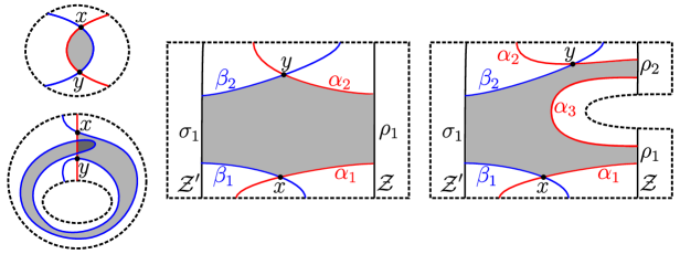
Figure 7. Some polygons. These are local pictures, that is, only a part of the diagram is shown (the boundary of which is indicated with dashed lines). Left: two polygons contributing to $n(x,y,(),())$, i.e., bigons. In the lower of the two, the darker region is covered with multiplicity two. Center: a polygon contributing to $n(x,y,(\rho_{1}),(\sigma_{1}))$. Right: a polygon contributing to $n(x,y,\allowbreak(\rho_{1},\rho_{2}),(\sigma_{1}))$.

Lemma 3.3.

Let $\mathcal{M}(x,y,(\sigma_{1},\dots,\sigma_{m}),(\rho_{1},\dots,\rho_{n}))$ be the moduli space of pseudoholomorphic curves as in [LOT10a] and [LOT11] connecting $x$ to $y$ with asymptotics specified by the sequences $(\sigma_{1},\dots,\sigma_{m}),(\rho_{1},\dots,\rho_{n})$. If this moduli space is $0$-dimensional then

$$n(x,y,(\sigma_{1},\dots,\sigma_{m}),(\rho_{1},\dots,\rho_{n}))\equiv\#\mathcal{M}(x,y,(\sigma_{1},\dots,\sigma_{m}),(\rho_{1},\dots,\rho_{n}))\pmod{2}.$$

Otherwise, $n(x,y,(\sigma_{1},\dots,\sigma_{m}),(\rho_{1},\dots,\rho_{n}))=0$.

Proof.

This follows from the definitions and the Riemann mapping theorem. ∎

Remark 3.4.

Counting immersed polygons in $\mathcal{D}(\phi)$ is combinatorial, and boils down to the combinatorics of gluing together components of $\mathcal{D}(\phi)\setminus({\boldsymbol{\alpha}}\cup{\boldsymbol{\beta}})$.

3.2. Type $D$ modules

The goal of this section is to associate a (differential) $\mathcal{C}(\mathcal{Z})$-bimodule $Q(\phi)$ to a strongly based mapping class $\phi\colon F(\mathcal{Z})\to F(\mathcal{Z})$. We first define a $\mathcal{C}(\mathcal{Z}^{\prime})$-$\mathcal{C}(\mathcal{Z})$-bimodule $P(\phi)$ associated to $\phi$, and then define $Q(\phi)$ in terms of $P(\phi)$.

Given a point $x\in{\boldsymbol{\alpha}}\cap{\boldsymbol{\beta}}$ define $I_{D}(x)$ to be the idempotent in $\mathcal{C}(\mathcal{Z}^{\prime})$ corresponding to the $\beta$-curves not occupied by $x$, and $J_{D}(x)$ to be the idempotent in $\mathcal{C}(\mathcal{Z})$ corresponding to the $\alpha$-curves not occupied by $x$. Let

$$P(\phi)=\bigoplus_{x\in{\boldsymbol{\alpha}}\cap{\boldsymbol{\beta}}}\mathcal{C}(\mathcal{Z}^{\prime})I_{D}(x)\otimes_{\mathbb{F}_{2}}J_{D}(x)\mathcal{C}(\mathcal{Z}).$$

This is a $\mathcal{C}(\mathcal{Z}^{\prime})$-$\mathcal{C}(\mathcal{Z})$-bimodule. Abusing notation imperceptibly, we let $x$ denote the generator for $P(\phi)$ corresponding to the intersection point $x$. Define a differential on $P(\phi)$ by

$$\partial(x)=\sum_{y\in{\boldsymbol{\alpha}}\cap{\boldsymbol{\beta}}}\sum_{\begin{subarray}{c}(\rho_{1},\dots,\rho_{n}),\\ (\sigma_{1},\dots,\sigma_{m})\end{subarray}}n(x,y,(\sigma_{1},\dots,\sigma_{m}),(\rho_{1},\dots,\rho_{n}))c(\sigma_{1})\cdot\cdots\cdot c(\sigma_{m})\cdot y\cdot c(\rho_{n})\cdot\cdots\cdot c(\rho_{1}),$$

and extending via the Leibniz rule $\partial(axb)=(\partial(a))xb+a(\partial(x))b+ax(\partial(b))$.

Lemma 3.5.

The bimodule $P(\phi)$ agrees with the bimodule $\widehat{\mathit{CFDD}}(\mathcal{D}(\phi),n/2-1)$ as defined in [LOT10a], [Zar09] and [LOT11].

Proof.

This is straightforward from the definitions and Lemma 3.3. (Note that in [LOT11] we would have thought of $P(\phi)$ as a left module over $\mathcal{C}(-\mathcal{Z})$ and a right module over $\mathcal{C}(-\mathcal{Z}^{\prime})$; using the fact that $\mathcal{C}(-\mathcal{Z})\cong\mathcal{C}(\mathcal{Z})^{\mathrm{op}}$ we are viewing $P(\phi)$ as a right module over $\mathcal{C}(\mathcal{Z})$ and left module over $\mathcal{C}(\mathcal{Z}^{\prime})$.) ∎

Proposition 3.6.

If $\phi$ is isotopic relative to the boundary of $F(\mathcal{Z})$ to $\psi$ then $P(\phi)$ is homotopy equivalent to $P(\psi)$.

Proof.

This follows from the identification $P(\phi)\cong\widehat{\mathit{CFDD}}(\mathcal{D}(\phi),n/2-1)$ (Lemma 3.5) and the corresponding invariance property of $\widehat{\mathit{CFDD}}(\mathcal{D}(\phi),\allowbreak n/2-1)$. (It should also be possible to give a direct proof, since all of the objects involved are topological.) ∎

The bimodules $P(\phi)$ are not the ones promised in the introduction; indeed, they are bimodules over two different algebras. We perform one further algebraic operation to them. Let $\mathbb{I}_{\mathcal{Z}}$ denote the identity map of $F(\mathcal{Z})$. Then for $\phi\in\mathit{MCG}_{0}(F(\mathcal{Z}))$ define

$$Q(\phi)=\operatorname{Mor}_{\mathcal{C}(\mathcal{Z}^{\prime})}(P(\mathbb{I}_{\mathcal{Z}}),P(\phi)),$$

where $\operatorname{Mor}$ denotes the chain complex of left module maps $P(\mathbb{I}_{\mathcal{Z}})\to P(\phi)$, which is a $\mathcal{C}(\mathcal{Z})$-bimodule.

Proposition 3.7.

The bimodule $Q(\phi)$ defined above agrees with the bimodule $\widehat{\mathit{CFDA}}(\phi,n/2-1)$ defined in [LOT10a] (or [Zar09]).

Proof.

The diagram $\mathcal{D}(\phi)$ is an $\alpha$-$\beta$-bordered Heegaard diagram. as in [LOT11]. On the other hand, $\mathcal{D}(\mathbb{I}_{-\mathcal{Z}})\cup_{\mathcal{Z}^{\prime}}\mathcal{D}(\phi)$ is an $\alpha$-$\alpha$-bordered Heegaard diagram for $\phi$, in the sense of [LOT10a]. Thus, the pairing theorem for bordered Floer homology expresses the bordered invariant $\widehat{\mathit{CFDA}}(\phi)$ as the $\mathcal{A}_{\infty}$ tensor product

(3.8) $$\widehat{\mathit{CFDA}}(\phi)\simeq\widehat{\mathit{CFAA}}(\mathcal{D}(\mathbb{I}_{-\mathcal{Z}}))\mathbin{\widetilde{\otimes}}_{\mathcal{A}(\mathcal{Z}^{\prime})}\widehat{\mathit{CFDD}}(\mathcal{D}(\phi)).$$

(See [LOT10a, Section 7] for the pairing theorem and, for instance, [Kel01] for a discussion of the $\mathcal{A}_{\infty}$ tensor product.) In particular, taking $\phi=\mathbb{I}$, the bimodules $\widehat{\mathit{CFDD}}(\mathcal{D}(\mathbb{I}_{\mathcal{Z}}))$ and $\widehat{\mathit{CFAA}}(\mathcal{D}(\mathbb{I}_{-\mathcal{Z}}))$ are quasi-inverses to each other (in the sense of [LOT10a, Definition LABEL:LOT2:def:QuasiInvertible]. So,

(3.9) $$\operatorname{Mor}_{\mathcal{A}(\mathcal{Z}^{\prime})}(\widehat{\mathit{CFDD}}(\mathcal{D}(\mathbb{I}_{\mathcal{Z}})),\mathcal{A}(\mathcal{Z}^{\prime}))\\ \begin{aligned} &\simeq\operatorname{Mor}_{\mathcal{A}(\mathcal{Z}^{\prime})}(\widehat{\mathit{CFAA}}(\mathcal{D}(\mathbb{I}_{-\mathcal{Z}}))\mathbin{\widetilde{\otimes}}\widehat{\mathit{CFDD}}(\mathcal{D}(\mathbb{I}_{\mathcal{Z}})),\widehat{\mathit{CFAA}}(\mathcal{D}(\mathbb{I}_{-\mathcal{Z}})))\\ &\simeq\widehat{\mathit{CFAA}}(\mathcal{D}(\mathbb{I}_{-\mathcal{Z}})).\end{aligned}$$

Combining Equations (3.8) and (3.9) and using the fact that $\widehat{\mathit{CFDD}}(\mathcal{D}(\phi),n/2-1)\cong P(\phi)$ gives the result. ∎

Corollary 3.10.

The bimodules $Q(\phi)$ satisfy the properties that $Q(\phi)\otimes Q(\psi)\simeq Q(\psi\circ\phi)$ and $Q(\mathbb{I})\simeq{}_{\mathcal{C}(\mathcal{Z})}\mathcal{C}(\mathcal{Z})_{\mathcal{C}(\mathcal{Z})}$. In particular, they give an action of $\mathit{MCG}_{0}(F(\mathcal{Z}))$ on the derived category of right differential modules over $\mathcal{C}(\mathcal{Z})$.

Proof.

This follows from Proposition 3.7 and the corresponding facts for $\widehat{\mathit{CFDA}}(\phi)$, which are proved in [LOT10a]. ∎

Remark 3.11.

The bimodules $Q(\phi)$ are left- and right-projective (compare [LOT10a, Corollary LABEL:LOT2:cor:tensor-projective]), so the ordinary tensor product in Corollary 3.10 agrees with the derived tensor product.

Example 3.12.

Figure 8 (left) shows a diagram for the identity map of the torus. There are three polygons (shown with different shadings in Figure 8 in the middle), contributing

$$\partial x_{1} =\sigma_{2,3}x_{2}\rho_{2,3}$$

$$\partial x_{2} =\sigma_{1,2}x_{1}\rho_{1,2}+\sigma_{3,4}x_{1}\rho_{3,4}$$

to the differential on $P(\mathbb{I})$. No other polygons contribute to the differential: for polygons to contribute in this case, their boundaries must contain a single connected segment in each of $\mathcal{Z}$ and $\mathcal{Z}^{\prime}$, with multiplicity one. Any polygon whose image is the union of two components of $\mathcal{D}(\mathbb{I})\setminus({\boldsymbol{\alpha}}\cup{\boldsymbol{\beta}})$ cannot contribute for idempotent reasons. The union of all three regions in $\mathcal{D}(\mathbb{I})\setminus({\boldsymbol{\alpha}}\cup{\boldsymbol{\beta}})$ is represented by two different polygons, one contributing to $n(x_{2},x_{1},(\sigma_{1,4}),(\rho_{3,4},\rho_{2,3},\rho_{1,2}))$ and one contributing to $n(x_{2},x_{1},\allowbreak(\sigma_{1,2},\sigma_{2,3},\sigma_{3,4}),\allowbreak(\rho_{1,4}))$. These cancel algebraically (each contributes $\sigma_{1,4}x_{1}\rho_{1,4}$ to $\partial x_{2}$).

Next, to compute $Q(\mathbb{I})$, we consider $\operatorname{Mor}_{\mathcal{C}(\mathcal{Z}^{\prime})}(P(\mathbb{I}),P(\mathbb{I}))$. As a left $\mathcal{C}(\mathcal{Z}^{\prime})$-module, $P(\mathbb{I})$ is generated by

$$S=\{x_{1},x_{1}\rho_{1,2},x_{1}\rho_{1,3},x_{1}\rho_{1,4},x_{1}\rho_{3,4},x_{2},x_{2}\rho_{2,3},x_{2}\rho_{2,4}\}.$$

Let $x$ be any element of $S_{1}=\{x_{1},x_{1}\rho_{1,2},x_{1}\rho_{1,3},x_{1}\rho_{1,4},x_{1}\rho_{3,4}\}$. Then there is an element in $\operatorname{Mor}_{\mathcal{C}(\mathcal{Z}^{\prime})}(P(\mathbb{I}),P(\mathbb{I}))$ sending $x$ to any element of

$$\{x_{1},x_{1}\rho_{1,2},x_{1}\rho_{1,3},x_{1}\rho_{1,4},x_{1}\rho_{3,4},\sigma_{2,4}x_{1},\sigma_{2,4}x_{1}\rho_{1,2},\sigma_{2,4}x_{1}\rho_{1,3},\sigma_{2,4}x_{1}\rho_{1,4},\\ \sigma_{2,4}x_{1}\rho_{3,4},\sigma_{2,3}x_{2},\sigma_{2,3}x_{2}\rho_{2,3},\sigma_{2,3}x_{2}\rho_{2,4}\}$$

and sending all other elements of $S$ to $0$.

Similarly, for $y$ any element of $S_{2}=\{x_{2},x_{2}\rho_{2,3},x_{2}\rho_{2,4}\}$ there is an element of $\operatorname{Mor}_{\mathcal{C}(\mathcal{Z}^{\prime})}(P(\mathbb{I}),\allowbreak P(\mathbb{I}))$ sending $y$ to any of

$$\{x_{2},x_{2}\rho_{2,3},x_{2}\rho_{2,4},\sigma_{1,3}x_{2},\sigma_{1,3}x_{2}\rho_{2,3},\sigma_{1,3}x_{2}\rho_{2,4},\\ \sigma_{1,2}x_{1},\sigma_{1,4}x_{1},\sigma_{3,4}x_{1},\sigma_{1,2}x_{1}\rho_{1,2},\sigma_{1,4}x_{1}\rho_{1,2},\sigma_{3,4}x_{1}\rho_{1,2},\sigma_{1,2}x_{1}\rho_{1,3},\sigma_{1,4}x_{1}\rho_{1,3},\sigma_{3,4}x_{1}\rho_{1,3},\\ \sigma_{1,2}x_{1}\rho_{1,4},\sigma_{1,4}x_{1}\rho_{1,4},\sigma_{3,4}x_{1}\rho_{1,4},\sigma_{1,2}x_{1}\rho_{3,4},\sigma_{1,4}x_{1}\rho_{3,4},\sigma_{3,4}x_{1}\rho_{3,4}\}$$

and sending all other elements of $S$ to $0$.

The next step in computing $Q(\mathbb{I})$ is to compute the differential and module structure on $\operatorname{Mor}_{\mathcal{C}(\mathcal{Z}^{\prime})}(P(\mathbb{I}),P(\mathbb{I}))$. This is cumbersome, although explicit. Some examples of this form can be found in [LOT11, Section 7] and [LOT10b, Section 8]. In Section 3.4 we will give a more practical way of working with one of our algebra actions.

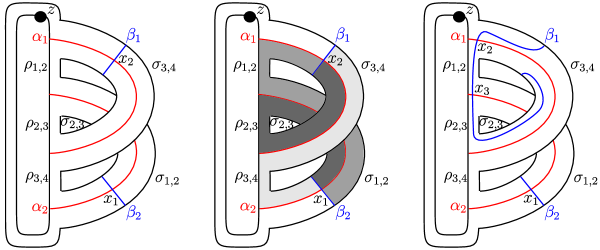
Figure 8. The identity map of the torus and a Dehn twist. Left: a diagram for the identity map of the torus. Center: three different polygons (rectangles) in the diagram, drawn with three different shadings. Right: a diagram for a Dehn twist around a particular essential curve in the torus.

Example 3.13.

Figure 8 on the right also shows a diagram for a particular Dehn twist of the torus. The associated module $P(\phi)$ has three generators, $x_{1}$, $x_{2}$ and $x_{3}$, with differentials

$$\partial(x_{1}) =\sigma_{2,3}x_{3}$$

$$\partial(x_{2}) =\sigma_{3,4}x_{1}\rho_{3,4}+x_{3}\rho_{1,2}$$

$$\partial(x_{3}) =\sigma_{1,2}x_{1}\rho_{1,3}+\sigma_{1,3}x_{2}\rho_{2,3}.$$

Unlike Example 3.12, where $\partial^{2}=0$ was forced by products in the algebra being zero, one of the cases of $\partial^{2}=0$ here involves cancellation:

$$\partial^{2}(x_{3})=\partial(\sigma_{1,2}x_{1}\rho_{1,3}+\sigma_{1,3}x_{2}\rho_{2,3})=\sigma_{1,2}\sigma_{2,3}x_{3}\rho_{1,3}+\sigma_{1,3}x_{3}\rho_{1,2}\rho_{2,3}=0.$$

3.3. Type $A$ modules

Let $M(\phi)$ be the ${\mathbb{F}_{2}}$-vector space generated by $\mathfrak{S}(\phi)={\boldsymbol{\alpha}}\cap{\boldsymbol{\beta}}$. We will make $M(\phi)$ into a ($\mathcal{A}_{\infty}$-) bimodule over $\mathcal{B}(\mathcal{Z}^{\prime})$ and $\mathcal{B}(\mathcal{Z})$. To start, define a left action of $\mathcal{B}(\mathcal{Z}^{\prime})$ and a right action of $\mathcal{B}(\mathcal{Z})$ on $M(\phi)$ as follows. Given $x\in\mathfrak{S}(\phi)$ and idempotents $I\in\mathcal{B}(\mathcal{Z}^{\prime})$, $J\in\mathcal{B}(\mathcal{Z})$ corresponding to arcs $\alpha_{i}$ and $\beta_{j}$ respectively, we have

$$I\cdot x\cdot J=\begin{cases}x&\text{if }x\in\alpha_{i}\cap\beta_{j}\\ 0&\text{otherwise.}\end{cases}$$

Next, given a chord $\rho$ in $\mathcal{B}(\mathcal{Z})$, define

$$x\cdot\rho=\sum_{y\in\mathfrak{S}(\phi)}n(x,y,(),(\rho))y.$$

Similarly, given a chord $\sigma$ in $\mathcal{B}(\mathcal{Z}^{\prime})$ and another point $y\in\mathfrak{S}(\mathcal{H})$, define

$$\sigma\cdot x=\sum_{y\in\mathfrak{S}(\phi)}n(x,y,(\sigma),())y.$$

We will also denote $\sigma\cdot x$ by $m_{1,1,0}(\sigma,x)$ and $x\cdot\rho$ by $m_{0,1,1}(x,\rho)$; the reason will become clear presently.

Example 3.14.

In the diagram for a Dehn twist of the torus in Figure 8, $x_{2}\rho_{1,2}=x_{3}$.

In general, the action we have defined so far may not be associative; see Figure 9. As the notation suggests, we should really think of $M(\phi)$ as an $\mathcal{A}_{\infty}$-bimodule. As a warm-up, define a differential on $M(\phi)$ by counting bigons:

$$\partial(x)=\sum_{y\in\mathfrak{S}(\phi)}n(x,y,(),())y.$$

It is straightforward to verify that $\partial^{2}=0$, and the reader to whom this is unfamiliar is encouraged to do so. We will also denote $\partial(x)$ as $m_{0,1,0}(x)$.

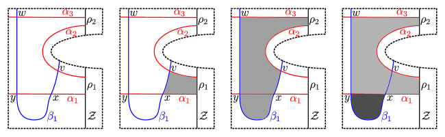
Figure 9. Non-associativity of the action on $M(\phi)$. This is a local example; only part of the diagram is drawn. There are products $x\cdot\rho_{1}=v$ and $v\cdot\rho_{2}=w$, given by the shaded regions in the second and third pictures, respectively. However, $x\cdot(\rho_{1}\rho_{2})=0$: there is (obviously) no rectangle giving a nontrivial operation of this form. The resolution is that $\partial(x)=y$ and $m_{3}(y,\rho_{1},\rho_{2})=w$; these operations are given by the darkly and lightly shaded regions in the fourth picture, respectively.

More generally, given a sequence of chords $\sigma_{1},\dots,\sigma_{n}$ in $\mathcal{B}(\mathcal{Z}^{\prime})$ and $\rho_{1},\dots,\rho_{n}$ in $\mathcal{B}(\mathcal{Z})$, and generators $x,y\in\mathfrak{S}(\phi)$ define

$$m_{m,1,n}(\sigma_{m},\dots,\sigma_{1},x,\rho_{1},\dots,\rho_{n})=\sum_{y\in\mathfrak{S}(\phi)}n(x,y,(\sigma_{1},\dots,\sigma_{m}),(\rho_{1},\dots,\rho_{n}))y.$$

Extend this multi-linearly to a map

$$m_{m,1,n}\colon\overbrace{\mathcal{B}(\mathcal{Z}^{\prime})\otimes\cdots\otimes\mathcal{B}(\mathcal{Z}^{\prime})}^{m\text{ copies}}\otimes M(\phi)\otimes\overbrace{\mathcal{B}(\mathcal{Z})\otimes\cdots\otimes\mathcal{B}(\mathcal{Z})}^{n\text{ copies}}\to M(\phi).$$

Lemma 3.15.

These $m_{i,1,j}$ endow $M(\phi)$ with the structure of an $\mathcal{A}_{\infty}$-bimodule.

Proof.

This is not too hard to prove combinatorially, but also follows from the analysis in [LOT08] and the Riemann mapping theorem. ∎

Remark 3.16.

Even if $m_{0,1,0}=0$, so that $m_{1,1,0}$ and $m_{0,1,1}$ make $M(\phi)$ into an honest bimodule, there is a lot of additional information in the higher $\mathcal{A}_{\infty}$-operations. See, for instance, Example 3.20.

As with the bimodules $P(\phi)$ in Section 3.2, the bimodules $M(\phi)$ are not the ones promised in the introduction. Let $\mathbb{I}_{\mathcal{Z}}$ denote the identity map of $F^{\circ}(\mathcal{Z})$. Then for $\phi\in\mathit{MCG}_{0}(F(\mathcal{Z}))$ define

(3.17) $$N(\phi)=\operatorname{Mor}_{\mathcal{B}(\mathcal{Z}^{\prime})}(M(\mathbb{I}_{\mathcal{Z}}),M(\phi)),$$

where $\operatorname{Mor}$ denotes the chain complex of left $\mathcal{A}_{\infty}$-module morphisms (whose cycles are the $\mathcal{A}_{\infty}$-homomorphisms); see, for instance, [LOT10a, Chapter 2]. Note that the right actions by $\mathcal{B}(\mathcal{Z})$ on $M(\mathbb{I})$ and $M(\phi)$ give $N(\phi)$ the structure of an ($\mathcal{A}_{\infty}$) $\mathcal{B}(\mathcal{Z})$-bimodule.

Proposition 3.18.

The bimodule $N(\phi)$ defined above agrees with the bimodule $\widehat{\mathit{CFDA}}(\phi,\allowbreak-n/2+1)$ defined in [LOT10a] (or [Zar09]).

Proof.

The proof is essentially the same as the proof of Proposition 3.7. ∎

Corollary 3.19.

The bimodules $N(\phi)$ satisfy the properties that $N(\phi)\mathbin{\widetilde{\otimes}}N(\psi)\simeq N(\psi\circ\phi)$ (where $\mathbin{\widetilde{\otimes}}$ denotes the $\mathcal{A}_{\infty}$ tensor product) and $N(\mathbb{I})\simeq{}_{\mathcal{B}(\mathcal{Z})}\mathcal{B}(\mathcal{Z})_{\mathcal{B}(\mathcal{Z})}$. In particular, the bimodules $N(\phi)$ give an action of $\mathit{MCG}_{0}(F(\mathcal{Z}))$ on the $\mathcal{A}_{\infty}$-homotopy category of right $\mathcal{A}_{\infty}$-modules over $\mathcal{B}(\mathcal{Z})$.

Proof.

Similarly to Corollary 3.10, this follows from Proposition 3.18 and the corresponding facts for $\widehat{\mathit{CFDA}}(\phi)$, which are proved in [LOT10a]. ∎

Example 3.20.

For the identity map $\mathbb{I}$ of the torus, using the diagram from Figure 8 $M(\mathbb{I})$ has two generators $x_{1}$ and $x_{2}$. The differential and ordinary product are both trivial. There are, however, obvious higher products given by the rectangles in Figure 8, of the forms:

$$m_{3}(\sigma_{1,2},x_{2},\rho_{1,2}) =x_{1}$$

$$m_{3}(\sigma_{3,4},x_{2},\rho_{3,4}) =x_{1}$$

$$m_{3}(\sigma_{2,3},x_{1},\rho_{2,3}) =x_{2}.$$

This is not the end of the story; indeed, with only these products, $M(\mathbb{I})$ would not satisfy the $\mathcal{A}_{\infty}$-relations. For instance, there is an operation

$$m_{4}(\sigma_{2,3},\sigma_{1,2},x_{2},\rho_{1,3})=x_{2}.$$

To see this, consider the union of the regions abutting $\rho_{1,2}$ and $\rho_{2,3}$. Make a cut in this region from $x_{2}$ along the $\beta$-curve to the boundary. The result is a polygon, from $x_{2}$ to itself, through the chord $\rho_{1,3}$ on one boundary component and the chords $\sigma_{2,3}$ and $\sigma_{1,2}$ on the other boundary component. (This operation is also forced by the $\mathcal{A}_{\infty}$-relation.)

Similarly, there are higher products:

$$m_{5}(\sigma_{1,3},\sigma_{1,2},x_{2},\rho_{1,3},\rho_{1,2}) =x_{1}$$

$$m_{6}(\sigma_{2,3},\sigma_{1,3},\sigma_{1,2},x_{2},\rho_{1,3},\rho_{1,3}) =x_{2}$$

$$m_{7}(\sigma_{1,3},\sigma_{1,3},\sigma_{1,2},x_{2},\rho_{1,3},\rho_{1,3},\rho_{1,2}) =x_{1}$$

$$\vdots$$

$$m_{5}(\sigma_{3,4},\sigma_{2,3},\sigma_{1,2},x_{2},\rho_{1,4}) =x_{1}$$

$$m_{6}(\sigma_{2,4},\sigma_{2,3},\sigma_{1,2},x_{2},\rho_{1,4},\rho_{2,3}) =x_{2}$$

$$m_{7}(\sigma_{1,4},\sigma_{2,3},\sigma_{1,2},x_{2},\rho_{1,4},\rho_{2,3},\rho_{1,2}) =x_{1}$$

$$\vdots,$$

as well as several more infinite families, and similar infinite families starting from $x_{1}$.

It would be natural to compute $N(\mathbb{I})$ next, via Equation (3.17). This is tedious (and infinite); we will give a better method for computing $N(\phi)$ from $M(\phi)$ in the next section. In particular, by Corollary 3.25, we have written down enough of $M(\phi)$ to characterize $N(\phi)$ (as well as $M(\phi)$).

3.4. Practical computations

As Example 3.12 illustrates, computing the bimodules $Q(\phi)$ and $N(\phi)$ from the modules $P(\phi)$ and $M(\phi)$ is quite cumbersome, and computing the tensor products $Q(\phi_{1})\otimes Q(\phi_{2})$ or $N(\phi_{1})\mathbin{\widetilde{\otimes}}N(\phi_{2})$ would be even more so. In this section, we give a reformulation of the bimodules $N(\phi)$ which is better suited for computations. The key tool is the type DD bimodule associated to the diagram $\mathcal{D}(\mathbb{I})$ in the second to lowest $\operatorname{spin}^{c}$-structure. (The type DD bimodules we have worked with so far are in the second to highest $\operatorname{spin}^{c}$-structure.)

Call a chord in $\mathcal{B}(\mathcal{Z})$ short if it connects adjacent points in ${\mathbf{a}}$. Let $\mathsf{SC}(\mathcal{Z})$ denote the set of short chords in $\mathcal{Z}$. The diagram $\mathcal{D}(\mathbb{I}_{\mathcal{Z}})$ sets up a correspondence between $\mathsf{SC}(\mathcal{Z})$ and $\mathsf{SC}(\mathcal{Z}^{\prime})$ as follows: two chords correspond if they lie on the boundary of a single connected component of $\mathcal{D}(\mathbb{I}_{\mathcal{Z}})\setminus({\boldsymbol{\alpha}}\cup{\boldsymbol{\beta}})$. Given a short chord $\xi\in\mathsf{SC}(\mathcal{Z})$ let $\xi^{\prime}$ be the corresponding short chord in $\mathsf{SC}(\mathcal{Z}^{\prime})$.

Definition 3.21.

Given an arc diagram $\mathcal{Z}$, let $\mathit{DD}\bigl{(}{\textstyle\frac{\mathbb{I}}{2}}\bigr{)}$ denote the $\mathcal{B}(\mathcal{Z})\text{-}\mathcal{B}(\mathcal{Z}^{\prime})$-bimodule defined as follows. The bimodule $\mathit{DD}\bigl{(}{\textstyle\frac{\mathbb{I}}{2}}\bigr{)}$ has one generator $x_{i}$ for each matched pair $\{a_{i},a^{\prime}_{i}\}$ in $M$. Let $I(x_{i})$ be the idempotent in $\mathcal{B}(\mathcal{Z})$ corresponding to $\{a_{i},a^{\prime}_{i}\}$ and $J(x_{i})$ the idempotent in $\mathcal{B}(\mathcal{Z}^{\prime})$ corresponding to $\{a_{i},a^{\prime}_{i}\}$. Let

$$\mathit{DD}\bigl{(}{\textstyle\frac{\mathbb{I}}{2}}\bigr{)}=\bigoplus_{i}\mathcal{B}(\mathcal{Z})I(x_{i})\otimes J(x_{i})\mathcal{B}(\mathcal{Z}^{\prime}).$$

Abusing notation, we also let $x_{i}$ denote a generator of the summand corresponding to $x_{i}$. Define a differential on $\mathit{DD}\bigl{(}{\textstyle\frac{\mathbb{I}}{2}}\bigr{)}$ by

$$\partial(x_{i})=\sum_{j}\sum_{\xi\in\mathsf{SC}(\mathcal{Z})}I(x_{i})\cdot\xi\cdot x_{j}\cdot\xi^{\prime}\cdot J(x_{i}),$$

and extending via the Leibniz rule. (Note that most terms in the sum defining $\partial(x_{i})$ vanish for idempotent reasons.)

Proposition 3.22.

The bimodule $\mathit{DD}\bigl{(}{\textstyle\frac{\mathbb{I}}{2}}\bigr{)}$ is homotopy equivalent to $\widehat{\mathit{CFDD}}(\mathcal{D}(\mathbb{I}_{-\mathcal{Z}}),\allowbreak-n/2+1)$.

Proof.

The identification of generators is given as follows: the generator $x_{i}$ for $\mathit{DD}\bigl{(}{\textstyle\frac{\mathbb{I}}{2}}\bigr{)}$ corresponding to the matched pair $\{a_{i},a^{\prime}_{i}\}$ corresponds to the generator $\mathbf{x}\subset{\boldsymbol{\alpha}}\cap{\boldsymbol{\beta}}$ for $\widehat{\mathit{CFDD}}(\mathcal{D}(\mathbb{I}_{-\mathcal{Z}}))$ consisting of $\{\alpha_{j}\cap\beta_{j}\mid j\neq i\}$. Each term in the differential on $\mathit{DD}\bigl{(}{\textstyle\frac{\mathbb{I}}{2}}\bigr{)}$ corresponds to an embedded hexagon in $\mathcal{D}(\mathbb{I}_{-\mathcal{Z}})$, and hence corresponds to a term in the differential on $\widehat{\mathit{CFDD}}(\mathcal{D}(\mathbb{I}_{-\mathcal{Z}}),-n/2+1)$. So, it remains to show that there are no other terms in the differential on $\widehat{\mathit{CFDD}}(\mathcal{D}(\mathbb{I}_{-\mathcal{Z}}),-n/2+1)$. We will do this by showing that there are no other index $1$ positive domains whose boundaries in $\mathcal{Z}$ and $\mathcal{Z}^{\prime}$ are such that they can contribute to the differential.

Writing $\mathcal{D}(\mathbb{I}_{-\mathcal{Z}})=(F^{\circ}(\mathcal{Z}),{\boldsymbol{\alpha}},{\boldsymbol{\beta}})$, each component of $F(\mathcal{Z})\setminus({\boldsymbol{\alpha}}\cup{\boldsymbol{\beta}})$ is a hexagon, with two sides contained in ${\boldsymbol{\alpha}}$, two sides contained in ${\boldsymbol{\beta}}$, one side in $\mathcal{Z}$ and one side in $\mathcal{Z}^{\prime}$.

For a domain $B$ to contribute $a^{\prime}\cdot y\cdot a$ to $\partial x$ we must have

$$e(B)+n_{\mathbf{x}}(B)+n_{\mathbf{y}}(B)-\iota(a)-\iota(a^{\prime})=-1.$$

For generators $a\in\mathcal{B}(\mathcal{Z})$, we have $\iota(a)=0$ if $a$ is an idempotent and $-1/2$ if $a$ is not. All non-trivial domains in $\mathcal{D}(\mathbb{I}_{-\mathcal{Z}})$ intersect both $\mathcal{Z}$ and $\mathcal{Z}^{\prime}$, so $\iota(a)=\iota(a^{\prime})=-1/2$. Thus, for a domain $B$ to contribute, it must have

$$e(B)+n_{\mathbf{x}}(B)+n_{\mathbf{y}}(B)=0.$$

Fix generators $\mathbf{x}=\{x_{1},\dots,x_{2n-1}\}$ and $\mathbf{y}=\{y_{1},\dots,y_{2n-1}\}$ for $\mathit{DD}\bigl{(}{\textstyle\frac{\mathbb{I}}{2}}\bigr{)}$. Reordering $\mathbf{x}$ and $\mathbf{y}$ if necessary, we may assume $x_{i}=y_{i}$ for $i<2n-1$. There are two cases: either $x_{2n-1}=y_{2n-1}$ or $x_{2n-1}\neq y_{2n-1}$. For simplicity, we will treat these two cases separately.

Case 1. $x_{2n-1}=y_{2n-1}$. There is one point $p\in{\boldsymbol{\alpha}}\cap{\boldsymbol{\beta}}$ not appearing in $\mathbf{x}=\mathbf{y}$. Let $R_{1},\dots,R_{4}$ denote the four components of $F^{\circ}(\mathcal{Z})\setminus({\boldsymbol{\alpha}}\cup{\boldsymbol{\beta}})$ which have $p$ as a corner. Note that $R_{i}\neq R_{j}$ for $i\neq j$ unless $R_{i}$ contains a basepoint.

If $R$ is some component of $F^{\circ}(\mathcal{Z})\setminus({\boldsymbol{\alpha}}\cup{\boldsymbol{\beta}})$ other than $R_{1},\dots,R_{4}$ then

$$e(R)+n_{\mathbf{x}}(R)+n_{\mathbf{y}}(R)=-1/2+1=1/2.$$

By contrast, for the regions $R_{1},\dots,R_{4}$,

$$e(R_{i})=-1/2+1/2=0.$$

Thus, for any positive domain $B$, $e(B)+n_{\mathbf{x}}(B)+n_{\mathbf{y}}(B)\geq 0$, with equality if and only if $B$ is a linear combination of $R_{1},\dots,R_{4}$. Thus, for grading reasons, the only domains that could contribute in this case are linear combinations of $R_{1},\dots,R_{4}$. Because the algebra element on each side must be a single, connected chord, the multiplicity of each $R_{i}$ must be $0$ or $1$. So, the rest of the argument boils down to the combinatorics of gluing together $\leq 4$ hexagons, each with two boundary components labeled $\alpha$, two labeled $\beta$, one labeled $\mathcal{Z}$ and one labeled $\mathcal{Z}^{\prime}$, and gluing allowed along the $\alpha$- and $\beta$-boundary components.

If we number the $R_{i}$ counter-clockwise around $p$, say, with $R_{1}$ separated from $R_{2}$ by a $\beta$-arc then the only such linear combinations which could give domains in $\pi_{2}(\mathbf{x},\mathbf{y})$ are $R_{1}+R_{2}$, $R_{2}+R_{3}$, $R_{3}+R_{4}$, $R_{4}+R_{1}$ and $R_{1}+R_{2}+R_{3}+R_{4}$. If $R_{1}+R_{2}$ gives a domain then the chords in $\mathcal{Z}$ corresponding to $R_{1}$ and $R_{2}$ must be consecutive. Such a domain has no holomorphic representative compatible with the idempotents, as in Example 3.12. The cases $R_{2}+R_{3}$, $R_{3}+R_{4}$ and $R_{4}+R_{1}$ are similar. For $R_{1}+R_{2}+R_{3}+R_{4}$, it is not possible for the domain to have connected boundary in $\mathcal{Z}$ (or $\mathcal{Z}^{\prime}$).

Thus, no domains from this case contribute to the differential on $\widehat{\mathit{CFDD}}(\mathcal{D}(\mathbb{I}_{-\mathcal{Z}}))$.

Case 2. $x_{2n-1}\neq y_{2n-1}$. As before, all regions have $e(R)+n_{\mathbf{x}}(R)+n_{\mathbf{y}}(R)\geq 0$. Moreover, equality only occurs for regions containing both $x_{2n-1}$ and $y_{2n-1}$ on their boundaries. There can be at most three such regions not containing basepoints; Figure 8 (on the left) is the essentially unique case in which there are three. Let $R_{1},R_{2},R_{3}$ denote the three such regions (if three exist). The only linear combinations of $R_{1},R_{2},R_{3}$ giving domains in $\pi_{2}(\mathbf{x},\mathbf{y})$ with multiplicities $0$ or $1$ everywhere in $\mathcal{Z}$ and $\mathcal{Z}^{\prime}$ are $R_{1}$, $R_{2}$, $R_{3}$, and $R_{1}+R_{2}+R_{3}$. The cases $R_{1}$, $R_{2}$ and $R_{3}$ contribute terms that occur in the differential on $\mathit{DD}\bigl{(}{\textstyle\frac{\mathbb{I}}{2}}\bigr{)}$. If $R_{1}+R_{2}+R_{3}$ exists then its geometry is exactly as in the genus $1$ case (Figure 8). Thus, as in Example 3.12, there are two cancelling holomorphic representatives.

This concludes the proof of Proposition 3.22. ∎

Corollary 3.23.

The bimodule $\mathit{DD}\bigl{(}{\textstyle\frac{\mathbb{I}}{2}}\bigr{)}\mathbin{\widetilde{\otimes}}_{\mathcal{B}(\mathcal{Z}^{\prime})}M(\phi)$ is $\mathcal{A}_{\infty}$-homotopy equivalent to $N(\phi)$.

Proof.

This follows from Proposition 3.22 and the definitions, similarly to the proof of Proposition 3.18. ∎

We have been using the notation $\mathbin{\widetilde{\otimes}}$ to denote the $\mathcal{A}_{\infty}$ tensor product. The resulting chain complexes are almost always infinite-dimensional. For cases under consideration, however, there is a smaller model for the $\mathcal{A}_{\infty}$ tensor product, which we denote $\boxtimes$. We refer the reader to [LOT10a] for the definition.

Example 3.24.

Continuing Example 3.20, we are now in a position to compute the bimodule $N$ for the identity map of the torus. In this case, the bimodule $\mathit{DD}\bigl{(}{\textstyle\frac{\mathbb{I}}{2}}\bigr{)}$ has generators $w_{1}$ and $w_{2}$, with

$$\partial w_{1} =\rho_{2,3}w_{2}\sigma_{2,3}$$

$$\partial w_{2} =\rho_{1,2}w_{1}\sigma_{1,2}+\rho_{3,4}w_{1}\sigma_{3,4}.$$

(This is, not coincidentally, the same as the bimodule $P(\mathbb{I})$ from Example 3.12.) Taking the $\boxtimes$ tensor product with the bimodule $M(\mathbb{I})$ from Example 3.20, we get a bimodule with generators $w_{1}\otimes x_{1}$ and $w_{2}\otimes x_{2}$, and operations:

$$m_{2}(w_{2}\otimes x_{2},\rho_{1,2}) =\rho_{1,2}w_{1}\otimes x_{1} m_{2}(w_{2}\otimes x_{2},\rho_{3,4}) =\rho_{3,4}w_{1}\otimes x_{1}$$

$$m_{2}(w_{1}\otimes x_{1},\rho_{2,3}) =\rho_{2,3}w_{2}\otimes x_{2} m_{2}(w_{2}\otimes x_{2},\rho_{1,3}) =\rho_{1,3}w_{2}\otimes x_{2}$$

$$m_{2}(w_{1}\otimes x_{1},\rho_{2,4}) =\rho_{2,4}w_{1}\otimes x_{1} m_{2}(w_{2}\otimes x_{2},\rho_{1,4}) =\rho_{1,4}w_{1}\otimes x_{1}.$$

This is exactly the $\mathcal{B}(\mathcal{Z})$-bimodule $\mathcal{B}(\mathcal{Z})$—as we expected.

(The module is projectively generated on the left, like the type $D$ cases above. On the right, it is an $\mathcal{A}_{\infty}$-module, like the type $A$ cases.)

We show a few examples of how these operations arise. The operation $m_{2}(w_{2}\otimes x_{2},\rho_{1,4})=\rho_{1,4}w_{1}\otimes x_{1}$ comes from a diagram of the following form:

using the higher product $m_{3}(\sigma_{1,2},x_{2},\rho_{1,2})=x_{1}$.

The operation $m_{2}(w_{2}\otimes x_{2},\rho_{1,2})=\rho_{1,2}w_{1}\otimes x_{1}$ comes from a diagram of the following form:

using the higher product $m_{5}(\sigma_{3,4},\sigma_{2,3},\sigma_{1,2},x_{2},\rho_{1,4})=x_{1}$. See [LOT10a] for more details.

Note that although the bimodule $M(\mathbb{I})$ had infinitely many nontrivial operations, the bimodule $N(\mathbb{I})$ has only finitely many. This will be true in general; see the discussion of boundedness in [LOT10a]. (In the terminology there, all of the bimodules in this paper are left and right bounded.)

Corollary 3.25.

The module $N(\phi)$ is determined by the higher products

$$m_{m,1,n}(\sigma_{i_{1}},\dots,\sigma_{i_{m}},\mathbf{x},\rho_{j_{1}},\dots,\rho_{j_{n}})$$

on $M(\phi)$ where $\sigma_{i_{1}},\dots,\sigma_{i_{m}}$ are short chords such that $\sigma^{\prime}_{i_{m}}\cdots\sigma^{\prime}_{i_{1}}\neq 0$. (In particular, the $\sigma_{i_{k}}$ are distinct and their union is connected.)

Proof.

In the bimodule $\mathit{DD}\bigl{(}{\textstyle\frac{\mathbb{I}}{2}}\bigr{)}\boxtimes M(\phi)$, these are the only higher products which can lead to non-zero terms in the differential. ∎

Remark 3.26.

The bimodule $\mathit{DD}\bigl{(}{\textstyle\frac{\mathbb{I}}{2}}\bigr{)}$ corresponds to the Koszul duality between the algebras $\mathcal{A}(\mathcal{Z})$ and $\mathcal{A}(\mathcal{Z}^{\prime})$. See [LOT11, Section 8].

3.5. Equivalence of the two actions

The reader might wonder if the two actions we have defined are genuinely different. They are not:

Proposition 3.27.

There is an equivalence of categories $\mathcal{F}\colon\mathcal{D}^{b}({}_{\mathcal{B}(\mathcal{Z})}\mathsf{Mod})\to\mathcal{D}^{b}({}_{\mathcal{C}(\mathcal{Z})}\mathsf{Mod})$ intertwining the actions of the mapping class group of $F(\mathcal{Z})$, in the sense that the diagram

commutes.

Proof.

In [LOT10a], we construct bimodules ${}_{\mathcal{B}(\mathcal{Z})}\widehat{\mathit{CFDD}}(\mathbb{I})_{\mathcal{C}(\mathcal{Z})}$ and ${}_{\mathcal{C}(\mathcal{Z})}\widehat{\mathit{CFAA}}(\mathbb{I})_{\mathcal{B}(\mathcal{Z})}$ such that for any mapping class $\phi$ of $F(\mathcal{Z})$,

$${}_{\mathcal{C}(\mathcal{Z})}\widehat{\mathit{CFAA}}(\mathbb{I})_{\mathcal{B}(\mathcal{Z})}\mathbin{\widetilde{\otimes}}{}_{\mathcal{B}(\mathcal{Z})}N(\phi)_{\mathcal{B}(\mathcal{Z})}\mathbin{\widetilde{\otimes}}{}_{\mathcal{B}(\mathcal{Z})}\widehat{\mathit{CFDD}}(\mathbb{I})_{\mathcal{C}(\mathcal{Z})} \simeq{}_{\mathcal{C}(\mathcal{Z})}Q(\phi)_{\mathcal{C}(\mathcal{Z})}$$

$${}_{\mathcal{B}(\mathcal{Z})}\widehat{\mathit{CFDD}}(\mathbb{I})_{\mathcal{C}(\mathcal{Z})}\otimes{}_{\mathcal{C}(\mathcal{Z})}Q(\phi)_{\mathcal{C}(\mathcal{Z})}\mathbin{\widetilde{\otimes}}{}_{\mathcal{C}(\mathcal{Z})}\widehat{\mathit{CFAA}}(\mathbb{I})_{\mathcal{B}(\mathcal{Z})} \simeq{}_{\mathcal{B}(\mathcal{Z})}N(\phi)_{\mathcal{B}(\mathcal{Z})}$$

$${}_{\mathcal{B}(\mathcal{Z})}\widehat{\mathit{CFDD}}(\mathbb{I})_{\mathcal{C}(\mathcal{Z})}\mathbin{\widetilde{\otimes}}{}_{\mathcal{C}(\mathcal{Z})}\widehat{\mathit{CFAA}}(\mathbb{I})_{\mathcal{B}(\mathcal{Z})} \simeq{}_{\mathcal{B}(\mathcal{Z})}\mathcal{B}(\mathcal{Z})_{\mathcal{B}(\mathcal{Z})}$$

$${}_{\mathcal{C}(\mathcal{Z})}\widehat{\mathit{CFAA}}(\mathbb{I})_{\mathcal{B}(\mathcal{Z})}\mathbin{\widetilde{\otimes}}{}_{\mathcal{B}(\mathcal{Z})}\widehat{\mathit{CFDD}}(\mathbb{I})_{\mathcal{C}(\mathcal{Z})} \simeq{}_{\mathcal{C}(\mathcal{Z})}\mathcal{C}(\mathcal{Z})_{\mathcal{C}(\mathcal{Z})}.$$

So, tensoring with $\widehat{\mathit{CFAA}}(\mathbb{I}_{\mathcal{Z}})$ gives the desired functor. ∎

4. Faithfulness of the action

To verify that the action is faithful, we start by giving a geometric interpretation of the rank of $H_{*}(M(\phi))$ for $\phi\in\mathit{MCG}_{0}(F)$. By definition, the rank of $H_{*}(M(\phi))$ in the idempotent corresponding to $\alpha_{i}$ and $\beta_{j}$ is the Floer homology of $\alpha_{i}$ with $\beta_{j}$. This Floer homology has a well-known geometric interpretation in terms of intersection numbers:

Lemma 4.1.

Let $\alpha$ and $\beta$ be non-isotopic, essential curves in a surface $F$, so that $\partial\alpha\subset\partial F$, $\partial\beta\subset\partial F$, $\partial\alpha\cap\partial\beta=\emptyset$, and $\alpha$ intersects $\beta$ transversely. Let $\mathit{HF}(\alpha,\beta)$ denote the Floer homology of the pair $(\alpha,\beta)$. That is, $\mathit{HF}(\alpha,\beta)$ is the homology of the chain complex $\mathit{CF}(\alpha,\beta)$ generated (over ${\mathbb{F}_{2}}$) by $\alpha\cap\beta$ and whose differential counts pseudoholomorphic bigons (or, equivalently, equivalence classes of immersed bigons) between $\alpha$ and $\beta$. Then $\dim_{\mathbb{F}_{2}}(\mathit{HF}(\alpha,\beta))=i(\alpha,\beta)$.

Here $i(\alpha,\beta)$ is geometric intersection number of $\alpha$ and $\beta$: the minimal number of intersections between any two curves isotopic (relative to the boundary) to $\alpha$ and $\beta$. This minimal number is achieved by any curves $\alpha^{\prime}$ and $\beta^{\prime}$ intersecting transversely with no bigons between them.

Proof.

The Floer homology group $\mathit{HF}(\alpha,\beta)$ is an isotopy invariant of $\alpha$ and $\beta$. If $\alpha^{\prime}$ and $\beta^{\prime}$ are isotopic to $\alpha$ and $\beta$ and arranged so that the are no bigons between $\alpha^{\prime}$ and $\beta^{\prime}$ then $\mathit{CF}(\alpha^{\prime},\beta^{\prime})$ has no differential. Thus,

$$\dim_{\mathbb{F}_{2}}(\mathit{HF}(\alpha,\beta))=\dim_{\mathbb{F}_{2}}(\mathit{CF}(\alpha^{\prime},\beta^{\prime}))=|\alpha^{\prime}\cap\beta^{\prime}|=i(\alpha,\beta),$$

as desired. ∎

To prove faithfulness of the mapping class group action, it suffices to prove:

Theorem 2.

The bimodule $N(\phi)$ (respectively $Q(\phi)$) is quasi-isomorphic to ${}_{\mathcal{B}(\mathcal{Z})}\mathcal{B}(\mathcal{Z})_{\mathcal{B}(\mathcal{Z})}$ (respectively ${}_{\mathcal{C}(\mathcal{Z})}\mathcal{C}(\mathcal{Z})_{\mathcal{C}(\mathcal{Z})}$) if and only if $\phi$ is isotopic to the identity.

Proof.

We discuss $N(\phi)$ first. The functor $\operatorname{Mor}_{\mathcal{B}(-\mathcal{Z}^{\prime})}(M(\mathbb{I}_{\mathcal{Z}}),\cdot)$ gives an equivalence of categories, so it suffices to show that $M(\phi)\simeq M(\mathbb{I})$ implies $\phi\sim\mathbb{I}$. Let $I_{i}$ denote the idempotent corresponding to $\eta_{i}$ (or $\beta_{i}$) and $J_{i}$ the idempotent corresponding to $\alpha_{i}$. Then $I_{i}H_{*}(M(\phi))J_{j}$ is the Floer homology group $\mathit{HF}(\beta_{i},\alpha_{j})$ so, by Lemma 4.1,

$$\dim_{\mathbb{F}_{2}}I_{i}H_{*}(M(\phi))J_{j}=i(\beta_{i},\alpha_{j}).$$

Thus, if $M(\phi)\simeq M(\mathbb{I})$ then $i(\beta_{i},\alpha_{j})=\delta_{i,j}$ By Lemma 3.1, this implies that $\{\beta_{i}\}$ is isotopic to the set of dual curves $\{\eta_{i}\}$ (which are also the $\beta$-curves for the identity map). Thus, $\phi$ fixes the curves $\eta_{i}$ (up to isotopy). Since the complement of the $\eta_{i}$ is a union of disks, and $\phi$ does not permute these disks (since $\phi$ fixes the boundary of $F(\mathcal{Z})$), this implies that $\phi\sim\mathbb{I}$.

The statement about $Q(\phi)$ follows formally, since $Q(\phi)\simeq\widehat{\mathit{CFAA}}(\mathbb{I}_{\mathcal{Z}})\mathbin{\widetilde{\otimes}}N(\phi)\mathbin{\widetilde{\otimes}}\widehat{\mathit{CFDD}}(\mathbb{I}_{\mathcal{Z}})$, and tensoring with $\widehat{\mathit{CFAA}}(\mathbb{I})$ and $\widehat{\mathit{CFDD}}(\mathbb{I})$ give equivalences of categories. Alternatively, we can give essentially the same proof as above. Let $\mathcal{I}(\mathcal{Z})$ denote the subring of idempotents in $\mathcal{C}(\mathcal{Z})$. Then

$$I_{i}H_{*}(\mathcal{I}(-\mathcal{Z}^{\prime})\otimes_{\mathcal{C}(-\mathcal{Z}^{\prime})}P(\phi)\otimes_{\mathcal{C}(\mathcal{Z})}\mathcal{I}(\mathcal{Z}))J_{j}\cong\mathit{HF}(\beta_{i},\alpha_{j}).$$

(Here, $\mathcal{I}(\mathcal{Z})$ is a $\mathcal{C}(\mathcal{Z})$-algebra via the augmentation map $\mathcal{C}(\mathcal{Z})\to\mathcal{I}(\mathcal{Z})$ sending any non-idempotent element to $0$.) The rest of the proof is then the same. ∎

Proof of Theorem 1.

This is immediate from Theorem 2, together with the identification between $N(\phi)$ and $\widehat{\mathit{CFDA}}(\phi,-n/2+1)$ (Proposition 3.18). ∎

As a corollary, when we iterate a map, the ranks of the homology of the bimodules grow like the dilatation of a pseudo-Anosov map.

Corollary 4.2.

For $\phi$ a pseudo-Anosov mapping class with dilatation $\lambda$,

$$\lim_{n\to\infty}\sqrt[n]{\dim_{\mathbb{F}_{2}}H_{*}(N(\phi^{n}))}=\lim_{n\to\infty}\sqrt[n]{\dim_{\mathbb{F}_{2}}H_{*}(Q(\phi^{n}))}=\lambda.$$

Proof.

First consider the similar statement for $M(\phi^{n})$. By Lemma 4.1,

$$\dim_{\mathbb{F}_{2}}I_{i}H_{*}(M(\phi^{n}))J_{j}=i(\beta_{i},\alpha_{j})=i(\phi^{n}(\eta_{i}),\alpha_{j}).$$

It is a well-known that the intersection numbers in pseudo-Anosov maps grow exponentially with the iteration. More precisely,

(4.3) $$\lim_{n\to\infty}\frac{i(\phi^{n}(\eta_{i}),\alpha_{j})}{\lambda^{n}}=\mu_{s}(\eta_{i})\mu_{u}(\alpha_{j})$$

where $\mu_{s}$ and $\mu_{u}$ are, respectively, the transverse measures on the stable and unstable foliations of $\phi$, suitably normalized. (See, e.g., [FLP79, Theorem 12.2] for the theorem for surfaces with no boundary, or [FLP79, Theorem 11.5] for a related theorem in the case of a surface with boundary.)

For the statement of the corollary, we do not need the precise constants on the right-hand side of Equation (4.3), just that they are non-zero. But $\mu_{s}(\eta_{i})\neq 0$ for any pseudo-Anosov map, as otherwise the simple closed curve formed by connecting the endpoints of $\eta_{i}$ along $\partial F$ would be a reducing curve. (If $\eta_{i}$ connects two different boundary components, consider instead the curve formed by taking two copies of $\eta_{i}$ and connecting the endpoints the long way around $\partial F$.) Similarly, $\mu_{u}(\alpha_{j})\neq 0$, so by Equation (4.3), $i(\phi^{n}(\eta_{i}),\alpha_{j})$ grows as $\lambda^{n}$. The dimension $\dim_{\mathbb{F}_{2}}H_{*}(M(\phi^{n}))$ is a sum of such terms, so $\dim_{\mathbb{F}_{2}}H_{*}(M(\phi^{n}))$ grows as $\lambda^{n}$, as well.

By definition, $N(\phi^{n})\simeq\operatorname{Mor}_{\mathcal{B}(-\mathcal{Z}^{\prime})}(M(\mathbb{I}_{\mathcal{Z}}),M(\phi^{n}))$. Since $\mathcal{B}(-\mathcal{Z}^{\prime})$ and $M(\mathbb{I}_{\mathcal{Z}})$ are finite-dimensional, $\dim_{\mathbb{F}_{2}}H_{*}(N(\phi^{n}))\leq K\dim_{\mathbb{F}_{2}}H_{*}(M(\phi^{n}))$ for some constant $K$. Since $\operatorname{Mor}_{\mathcal{B}(-\mathcal{Z}^{\prime})}(M(\mathbb{I}_{\mathcal{Z}}),\cdot)$ is an equivalence of categories (with inverse given by taking $\operatorname{Mor}$ with another bimodule), we also have a similar bound the other direction, proving the statement in the corollary for $N(\phi^{n})$.

The statement about $Q(\phi)$ follows similarly, since $Q(\phi)\simeq\widehat{\mathit{CFAA}}(\mathbb{I}_{\mathcal{Z}})\mathbin{\widetilde{\otimes}}N(\phi)\mathbin{\widetilde{\otimes}}\widehat{\mathit{CFDD}}(\mathbb{I}_{\mathcal{Z}})$, and both $\widehat{\mathit{CFAA}}(\mathbb{I}_{\mathcal{Z}})$ and $\widehat{\mathit{CFDD}}(\mathbb{I}_{\mathcal{Z}})$ are finite-dimensional, and tensoring with $\widehat{\mathit{CFAA}}(\mathbb{I}_{\mathcal{Z}})$ (respectively $\widehat{\mathit{CFDD}}(\mathbb{I}_{\mathcal{Z}})$) gives an equivalence of categories (where tensoring with $\widehat{\mathit{CFDD}}(\mathbb{I}_{\mathcal{Z}})$ (respectively $\widehat{\mathit{CFAA}}(\mathbb{I}_{\mathcal{Z}})$) gives the inverse equivalence). ∎

Remark 4.4.

A similar statement holds if $\phi$ is reducible; then the growth rate of the rank of the homology is given by the maximum dilatation of any pseudo-Anosov component of $\phi$, as at least one $\alpha_{i}$ and one $\eta_{j}$ must intersect the pseudo-Anosov component. If $\phi$ has no pseudo-Anosov components (i.e., some power of $\phi$ is a composition of Dehn twists along pairwise-disjoint curves), the rank of the homology grows only linearly.

5. Finite generation

In this section, we briefly review the sense in which the module categories on which the mapping class group is acting are finitely generated.

Definition 5.1.

Given objects $\{M_{i}\}$ in triangulated category $\mathscr{C}$, the subcategory generated by $\{M_{i}\}$ is the smallest triangulated subcategory of $\mathscr{C}$ containing all of the $M_{i}$. We say that $\{M_{i}\}$ generate $\mathscr{C}$ if the subcategory generated by $\{M_{i}\}$ is, in fact, $\mathscr{C}$. We say that $\mathscr{C}$ is finitely generated if there is a finite set of objects $\{M_{i}\}$ which generate $\mathscr{C}$.

Although the definition of finite generation is rather abstract, our proof that our module categories are finitely generated will be satisfyingly concrete. Fix an arc diagram $\mathcal{Z}$, and let $\mathcal{B}=\mathcal{B}(\mathcal{Z})$, $\mathcal{C}=\mathcal{C}(\mathcal{Z})$. Before giving the proof, we develop a little more algebra. Let $\mathcal{C}_{+}$ be the ideal in $\mathcal{C}$ generated by all strand diagrams $s$ in which not all strands are horizontal (so as an ${\mathbb{F}_{2}}$-vector space, $\mathcal{C}$ is the direct sum of $\mathcal{C}_{+}$ and the subring of idempotents of $\mathcal{C}$). Observe that $\mathcal{C}_{+}$ is nilpotent; for instance, this follows from the facts that $\mathcal{C}$ is finite-dimensional, the total length gives a grading on $\mathcal{C}$, and $\mathcal{C}_{+}$ is the positively graded part of $\mathcal{C}$ with respect to this grading (compare Remark 2.15). In particular, for any $\mathcal{C}$-module $M$, the module $\mathcal{C}_{+}\cdot M$ is a proper submodule of $M$.

A simple module over $\mathcal{C}$ is a module $M$ which is $1$-dimensional over ${\mathbb{F}_{2}}$ (and so has trivial differential). The simple modules are in bijective correspondence with the $2n$ minimal idempotents in $\mathcal{C}$.

Theorem 3.

The derived categories $\mathcal{D}^{b}({}_{\mathcal{B}}\mathsf{Mod})$ and $\mathcal{D}^{b}({}_{\mathcal{C}}\mathsf{Mod})$ are finitely generated.

Proof.

We start by proving the statement for $\mathcal{D}^{b}({}_{\mathcal{C}}\mathsf{Mod})$; one can give a similar proof for $\mathcal{B}$, but since we have been working with $\mathcal{A}_{\infty}$-modules over $\mathcal{B}$ a little extra verbiage is required.

We prove that $\mathcal{C}$ is generated by the simple modules. Our proof is by induction on the dimension over ${\mathbb{F}_{2}}$ of a differential module $M\in\mathcal{D}^{b}({}_{\mathcal{C}}\mathsf{Mod})$. There is a short exact sequence

$$0\to\mathcal{C}_{+}M\to M\to M/(\mathcal{C}_{+}M)\to 0.$$

Further, $M/\mathcal{C}_{+}M$ is a direct sum of simple modules and $\mathcal{C}_{+}M$ has strictly smaller dimension than $M$. By induction, we can assume that $\mathcal{C}_{+}M$ is in the triangulated subcategory generated by the simple modules; it follows that $M$ is in this subcategory as well.

The statement for $\mathcal{D}^{b}({}_{\mathcal{B}}\mathsf{Mod})$ now follows from the statement for $\mathcal{D}^{b}({}_{\mathcal{C}}\mathsf{Mod})$ and the fact that tensoring with $\widehat{\mathit{CFAA}}(\mathbb{I})$ gives an equivalence between the two categories. ∎

Remark 5.2.

If we prefer to think of elements of $\mathcal{D}^{b}({}_{\mathcal{C}}\mathsf{Mod})$ as projective modules, we can give a similar proof using the elementary projective modules $\mathcal{C}\cdot I$ (for $I$ one of the $n$ minimal idempotents).

It is not hard to extend the proof of Theorem 3 to give the following:

Theorem 4.

The modulo $2$ Grothendieck group $G({}_{\mathcal{B}}\mathsf{Mod})$ of differential $\mathcal{B}$-modules is isomorphic to $H_{1}(F(\mathcal{Z});\mathbb{Z}/2)$. The action of the mapping class group on ${}_{\mathcal{B}}\mathsf{Mod}$ defined in this paper decategorifies to the standard action of the mapping class group on $H_{1}(F(\mathcal{Z});\mathbb{Z}/2)$. The corresponding statements also hold for ${}_{\mathcal{C}}\mathsf{Mod}$, as well as for the Grothendieck groups of projective differential modules $K_{0}({}_{\mathcal{B}}\mathsf{Mod})$ and $K_{0}({}_{\mathcal{C}}\mathsf{Mod})$.

Proof.

The proof of Theorem 3 shows that the $n$ elementary modules generate $G({}_{\mathcal{C}}\mathsf{Mod})$. To see that they are linearly independent, consider the algebra map

$$\mathcal{C}\to\mathcal{C}/\mathcal{C}_{+}=\bigoplus_{i=1}^{n}{\mathbb{F}_{2}}.$$

This maps the $n$ generators of $G({}_{\mathcal{C}}\mathsf{Mod})$ to a basis for $G({}_{\mathcal{C}/\mathcal{C}_{+}}\mathsf{Mod})=({\mathbb{F}_{2}})^{n}$.

To understand the induced mapping class group action, let $\alpha_{1},\dots,\alpha_{n}$ be the basis of curves for $F(\mathcal{Z})$ specified by the pairs of points in $M$, and let $\gamma_{1},\dots,\gamma_{n}$ be dual curves. Then, for idempotents $I_{i}$ and $I_{j}$, the number of generators $g_{ij}$ of $I_{i}\widehat{\mathit{CFDA}}(\phi,-n/2+1)I_{j}$ (as a type DA bimodule) is equal (modulo $2$) to the number of intersections between $\phi(\alpha_{i})$ and $\gamma_{j}$. (To see this, note that each generator of $N(\phi)$ can be promoted uniquely to a generator of $\widehat{\mathit{CFDA}}(\phi,-n/2+1)$.) Use the $\alpha_{i}$ to give a basis $[\alpha_{1}],\dots,[\alpha_{n}]$ for $H_{1}(F(\mathcal{Z}))$. With respect to this basis,

$$\phi_{*}[\alpha_{i}] =(\alpha_{i}\cdot\gamma_{1},\dots,\alpha_{i}\cdot\gamma_{n})$$

$$\equiv(g_{i,1},\dots,g_{i,n})\pmod{2}.$$

This implies that the induced action on Grothendieck groups agrees with the action on $H_{1}(F(\mathcal{Z}))$.

The results for $G({}_{\mathcal{B}}\mathsf{Mod})$, $K_{0}({}_{\mathcal{B}}\mathsf{Mod})$ and $K_{0}({}_{\mathcal{C}}\mathsf{Mod})$ follow similarly; alternatively, they follow from the fact that all of these triangulated categories are equivalent. ∎

Remark 5.3.

Since we have been working with ungraded differential modules, we are forced to use the modulo $2$ Grothendieck groups in Theorem 4.

Remark 5.4.

The proof of Theorem 4 immediately extends to show that the action of the mapping class group on $G({}_{\mathcal{A}(\mathcal{Z})}\mathsf{Mod})\cong\Lambda^{*}H_{1}(F(\mathcal{Z});\mathbb{Z}/2)$ is the standard action on $\Lambda^{*}H_{1}(F(\mathcal{Z});\mathbb{Z}/2)$.

Remark 5.5.

In light of Auroux’s reformulation of bordered Floer theory in terms of partially-wrapped Fukaya categories [Aur10], it is natural to compare Theorem 4 with Abouzaid’s computation of the Grothendieck group of modules over the Fukaya category of a closed surface [Abo08]: for the Fukaya category of a closed surface $F$, the Grothendieck group is $H_{1}(SF;\mathbb{Z})\bigoplus\mathbb{R}$, where $SF$ is the unit tangent bundle to $F$.

6. Further questions

The results of this paper suggest several natural questions. Most prominent among them is whether knowing that the mapping class group has a faithful representation on a linear category has group-theoretic consequences. A faithful action of a group on a vector space has many consequences (like the Tits alternative [Tit72] and residual finiteness), and many of these consequences are known to hold for mapping class groups. It seems plausible that some of these could be explained by the linear-categorical actions of the mapping class groups.

A second natural question is whether one can give a similar linear-categorical action of the mapping class group of a closed surface.

A question more internal to Heegaard Floer homology is whether the actions on bordered Floer homology in $\operatorname{spin}^{c}$-structures between the $(-n/2+1)^{\text{st}}$ and $(n/2-1)^{\text{st}}$ are faithful. It seems likely that they are, but the techniques of this paper do not apply directly.

Finally, there are many known categorical actions of braid groups. It would be interesting to know which, if any, of these admit extensions to mapping class group actions; in particular, this would be a step towards extending Khovanov-type knot invariants to $3$-manifold invariants.

References

- [Abo08] Mohammed Abouzaid, On the Fukaya categories of higher genus surfaces, Adv. Math. 217 (2008), no. 3, 1192–1235.
- [AGW11] Denis Auroux, J. Elisenda Grigsby, and Stephan Wehrli, On Khovanov-Seidel quiver algebras and bordered Floer homology, 2011, arXiv:1107.2841.
- [Aur10] Denis Auroux, Fukaya categories of symmetric products and bordered Heegaard-Floer homology, J. Gökova Geom. Topol. 4 (2010), 1–54, arXiv:1001.4323.
- [FLP79] A. Fathi, F. Laundenbach, and V. Poénaru (eds.), Travaux de Thurston sur les surfaces, Astérisque, vol. 66, Société Mathématique de France, Paris, 1979, Séminaire Orsay, with an English summary.
- [GW10] J. Elisenda Grigsby and Stephan M. Wehrli, On the colored Jones polynomial, sutured Floer homology, and knot Floer homology, Adv. Math. 223 (2010), no. 6, 2114–2165, arXiv:0907.4375.
- [Kel01] Bernhard Keller, Introduction to -infinity algebras and modules, Homology Homotopy Appl. 3 (2001), no. 1, 1–35, arXiv:math.RA/9910179.
- [KM11] Peter B. Kronheimer and Tomasz Mrowka, Khovanov homology is an unknot-detector, Publ. Math. Inst. Hautes Études Sci. (2011), no. 113, 97–208, arXiv:1005.4346.
- [KS02] Mikhail Khovanov and Paul Seidel, Quivers, Floer cohomology, and braid group actions, J. Amer. Math. Soc. 15 (2002), no. 1, 203–271, arxiv:math.QA/0006056.
- [KT07] Mikhail Khovanov and Richard Thomas, Braid cobordisms, triangulated categories, and flag varieties, Homology Homotopy Appl. 9 (2007), no. 2, 19–94, arXiv:math/0609335.
- [LOT08] Robert Lipshitz, Peter S. Ozsváth, and Dylan P. Thurston, Bordered Heegaard Floer homology: Invariance and pairing, 2008, arXiv:0810.0687v4.
- [LOT10a] by same author, Bimodules in bordered Heegaard Floer homology, 2010, arXiv:1003.0598v3.
- [LOT10b] by same author, Computing by factoring mapping classes, 2010, arXiv:1010.2550v3.
- [LOT11] Robert Lipshitz, Peter S. Ozsváth, and Dylan P. Thurston, Heegaard Floer homology as morphism spaces, Quantum Topology 2 (2011), no. 4, 384–449, arXiv:1005.1248.
- [Sei02] Paul Seidel, Symplectic Floer homology and the mapping class group, Pacific J. Math. 206 (2002), no. 1, 219–229.
- [Sie11] Kyler Siegel, A geometric proof of a faithful linear-categorical surface mapping class group action, 2011, arXiv:1108.3676.
- [Tit72] J. Tits, Free subgroups in linear groups, J. Algebra 20 (1972), 250–270.
- [Zar09] Rumen Zarev, Bordered Floer homology for sutured manifolds, 2009, arXiv:0908.1106.