63ème année, 2010-2011 1028

Sieve in expansion

1 Introduction

This report presents recent works extending sieve methods, from their classical setting, to new situations characterized by the targeting of sets with exponential growth, arising often from discrete groups like $\operatorname{SL}_{m}(\mathbf{Z})$ or sufficiently big subgroups.

A recent lecture of Sarnak [54] mentions some of the original motivation (related to the Markov equation and closed geodesics on the modular surface). The first general results concerning these sieve problems appeared around $2005$ in preprint form, and Bourgain, Gamburd and Sarnak have written a basic paper presenting its particular features [4]. Other applications, with a very different geometric flavor, also appeared independently around that time, first (somewhat implicitly) in some works of Rivin [52].

The most crucial feature in applying sieve to these new situations is their dependence on spectral gaps, either in a discrete setting (related to expander graphs or to Property $(\tau)$ of Lubotzky [40]) or in a geometric setting (generalizing for instance Selberg’s result that $\lambda_{1}\geqslant 3/16$ for the spectrum of the Laplace operator on the classical hyperbolic modular surfaces).

The outcome of these developments is that there now exist very general sieve inequalities involving, roughly speaking, discrete objects with exponential growth. Moreover, their applicability (including to problems seemingly unrelated with classical analytic number theory, as we will show) has expanded enormously, as – partly motivated by these new applications of sieve methods – many new cases of spectral gaps have become available. Particularly impressive are the results on expansion in finite linear groups (due to many people, but starting from the breakthrough of Helfgott [26] for $\operatorname{SL}_{2}$), and those concerning applications of ergodic methods to lattices in semisimple groups with Property $(\tau)$ (developed most generally by Gorodnik and Nevo [21]).

Before going towards the heart of this report, we state here a particularly concrete and appealing result arising from sieve in expansion. We recall first that $\Omega(n)$ is the arithmetic function giving the number of prime factors, counted with multiplicity, of a non-zero integer $n$, extended so that $\Omega(0)=+\infty$.

Let $\Lambda\subset\operatorname{SL}_{m}(\mathbf{Z})$ be a Zariski-dense subgroup, for instance the group $L$ generated by the elements

$$\begin{pmatrix}1&\pm 3\\ 0&1\end{pmatrix},\quad\begin{pmatrix}1&0\\ \pm 3&1\end{pmatrix}\in\operatorname{SL}_{2}(\mathbf{Z}),$$ (1)

in the case $m=2$

Let $f$ be an integral polynomial function on $\mathbf{Z}^{m}$, which is non-constant. Let $x_{0}\in\mathbf{Z}^{m}-\{0\}$ be a fixed vector. There exists an integer $r=r(f,x_{0},\Lambda)\geqslant 1$ such that the set

$$\mathcal{O}_{f}(x_{0};r)=\{\gamma\in\Lambda\,\mid\,\Omega(f(\gamma\cdot x_{0}))\leqslant r\}$$

is Zariski-dense in $\operatorname{SL}_{m}$, and in particular is infinite. In fact, there exists such $r$ for which $\mathcal{O}_{f}(x_{0};r)$ is not thin, in the sense of [57, Def. 3.1.1].

Part of the point, and it will be emphasized below, is that $\Lambda$ may have infinite index in $\operatorname{SL}_{m}(\mathbf{Z})$. In particular, for $m=2$, this is the case for the group $L$ generated by the matrices (1).

Notation. We recall here some basic notation.

– The letter $p$ will always refer to prime numbers; for a prime $p$, we write $\mathbf{F}_{p}$ for the finite field $\mathbf{Z}/p\mathbf{Z}$, and we write $\mathbf{F}_{q}$ for a field with $q$ elements. For a set $X$, $|X|$ is its cardinality, a non-negative integer or $+\infty$.

– The Landau and Vinogradov notation $f=O(g)$ and $f\ll g$ are synonymous, and $f(x)=O(g(x))$ for all $x\in D$ means that there exists an “implied” constant $C\geqslant 0$ (which may be a function of other parameters, explicitly mentioned) such that $|f(x)|\leqslant Cg(x)$ for all $x\in D$. This definition differs from that of N. Bourbaki [1, Chap. V] since the latter is of topological nature. On the other hand, the notation $f(x)\sim g(x)$ and $f=o(g)$ are used with the asymptotic meaning of loc. cit.

Acknowledgments. Thanks are due to J. Bourgain, N. Dunfield, E. Fuchs, A. Gamburd, F. Jouve, A. Kontorovich, H. Oh, L. Pyber, P. Sarnak, D. Zywina and others for their help, remarks and corrections concerning this report. In particular, discussions with O. Marfaing during his preparation of a Master Thesis on this topic [43] were very helpful.

2 Motivation

Sieve methods are concerned with multiplicative properties of sets of integers. Thus to expand the range of the sieve, one should describe new sets of integers to investigate. To present the spirit of this survey, we first give two examples of such sets of integers, which are rather unusual from a sieve perspective. One of them is a particularly appealing instance of “sieve in orbits”, first considered in [4]: the distribution of curvatures of integral Apollonian circle packings. The second is even more surprising to look at: it has to do with the first homology of certain “random” $3$-manifolds. Although we will say rather less about it later on, it presents some unusual features, and suggests interesting questions.

2.1 Apollonian circle packings

It is a very classical geometrical fact that, given three circles $(\bigcirc_{1},\bigcirc_{2},\bigcirc_{3})$ in the plane which are pairwise tangent to each other, and have disjoint “interiors” (the discs they bound), with radii $(r_{1},r_{2},r_{3})$ and curvatures $(c_{1},c_{2},c_{3})=(r_{1}^{-1},r_{2}^{-1},r_{3}^{-1})$, one can find two more circles (say $(\bigcirc_{4},\bigcirc^{\prime}_{4})$ with curvatures $(c_{4},c^{\prime}_{4})$), so that both

$$(\bigcirc_{1},\bigcirc_{2},\bigcirc_{3},\bigcirc_{4})\text{ and }(\bigcirc_{1},\bigcirc_{2},\bigcirc_{3},\bigcirc^{\prime}_{4})$$

are four pairwise tangent circles (with disjoint “interiors”). In fact, this applies also to negative radii or curvatures, where a negative radius is interpreted to mean that the “interior” of the circle should be the complement of the bounded disc (see Figure 1). Such $4$-tuples are called Descartes configurations, since a result of Descartes states that the two sets of four curvatures satisfy the quadratic equations

$$Q(c_{1},c_{2},c_{3},c_{4})=Q(c_{1},c_{2},c_{3},c^{\prime}_{4})=0$$

where

$$Q(x,y,z,t)=2(x^{2}+y^{2}+z^{2}+t^{2})-(x+y+z+t)^{2}.$$

In particular, if $(\bigcirc_{1},\bigcirc_{2},\bigcirc_{3},\bigcirc_{4})$ are such that their curvatures are all integers, then we obtain an integral quadratic equation for $c^{\prime}_{4}$ where one solution (namely, $c_{4}$) is an integer: thus $c^{\prime}_{4}$ is an integer also. Moreover, again given $(\bigcirc_{1},\bigcirc_{2},\bigcirc_{3},\bigcirc_{4})$ with integral curvatures, there are also circles

$$\bigcirc^{\prime}_{1},\bigcirc^{\prime}_{2},\bigcirc^{\prime}_{3},$$

for which, for instance, the circles

$$(\bigcirc^{\prime}_{1},\bigcirc_{2},\bigcirc_{3},\bigcirc_{4})$$

form a Descartes configuration, and as above, the curvatures $c^{\prime}_{1}$, $c^{\prime}_{2}$, $c^{\prime}_{3}$ are integers. In fact, these new curvatures are given – by solving the quadratic equation using the known root – as

$$(c^{\prime}_{1},c_{2},c_{3},c_{4})=(c_{1},c_{2},c_{3},c_{4})\cdot{}^{t}{{s_{1}}},$$

$$(c_{1},c^{\prime}_{2},c_{3},c_{4})=(c_{1},c_{2},c_{3},c_{4})\cdot{}^{t}{{s_{2}}},$$

$$(c_{1},c_{2},c^{\prime}_{3},c_{4})=(c_{1},c_{2},c_{3},c_{4})\cdot{}^{t}{{s_{3}}},$$

$$(c_{1},c_{2},c_{3},c^{\prime}_{4})=(c_{1},c_{2},c_{3},c_{4})\cdot{}^{t}{{s_{4}}},$$

where the matrices $s_{1}$, …, $s_{4}$ are in the group $O(Q,\mathbf{Z})$ of integral automorphisms of the quadratic form above, namely

$$s_{1}=\begin{pmatrix}-1&2&2&2\\ &1&&\\ &&1&\\ &&&1\end{pmatrix},\quad\quad s_{2}=\begin{pmatrix}1&&&\\ 2&-1&2&2\\ &&1&\\ &&&1\end{pmatrix},\quad\quad$$

and $s_{3}$ and $s_{4}$ are similar. Note that $s_{i}^{2}=1$ for all $i$, and one can in fact show that these are the only relations satisfied by those matrices.

Each of the new sets of curvatures can be used to iterate the process; in other words, denoting by $\mathcal{A}$ the subgroup of $O(Q,\mathbf{Z})$ generated by the $s_{i}$, the integers arising as coefficients of a vector in the orbit $\mathcal{A}\cdot\text{\boldmath${c}$}$ of a “root quadruple” $\text{\boldmath${c}$}=(c_{1},\ldots,c_{4})$, are all the curvatures of circles arising in this iterative circle packing. These are Apollonian circle packings, and the first step is described in Figure 1 in one particular case (where one notices the convention dealing with negative curvatures).

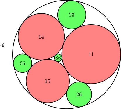
Figure 1: Apollonian circle packing for $\text{\boldmath${c}$}=(-6,11,14,15)$; the labels are the curvatures.

The set $\mathcal{C}(\text{\boldmath${c}$})$ of these curvatures, considered with or without multiplicity, is our first example of integers to sieve for. It is clear from the outset that such an attempt will be deeply connected with the understanding of the group $\mathcal{A}$. Moreover, an interest in the multiplicative properties of the elements of $\mathcal{C}(\text{\boldmath${c}$})$ will obviously depend on the properties of the reduction maps

$$\mathcal{A}\rightarrow\mathcal{A}_{p}=\mathcal{A}\ (\mathrm{mod}\ {{p}})\subset O(Q,\mathbf{Z}/p\mathbf{Z}),$$

modulo primes, and in particular in the image of this reduction map.

The following features of $\mathcal{A}$ illustrate a basic property that makes the question challenging:

– The group $\mathcal{A}$ is “big” in some sense: it is Zariski-dense in $O(Q)$ (as a $\mathbf{Q}$-algebraic group), so that, if one can only use polynomial constructions, $\mathcal{A}$ is indistinguishable from the big Lie group $O(Q,\mathbf{C})$.

– However, $\mathcal{A}$ is “small” in some other sense: specifically, $\mathcal{A}$ has infinite index in $O(Q,\mathbf{Z})$. Stated differently, the quotient $\mathcal{A}\backslash O(Q,\mathbf{R})$ (a three-manifold) has infinite volume for its natural measure, induced from Haar measure on $O(Q,\mathbf{R})$.

Arithmetic properties of Apollonian packings were first discussed in [23], including some properties of $\mathcal{C}(\text{\boldmath${c}$})$; the use of sieve to study $\mathcal{C}(\text{\boldmath${c}$})$ was begun in [4].

2.2 Dunfield-Thurston random $3$-manifolds

Our second example of integers to sieve from is chosen partly as an illustration of the great versatility of sieve, and partly because it will lead to some interesting examples later. It is based on a paper of Dunfield and Thurston [13] (which did not explicitly introduce sieve); related work is due to Maher [42] and the author [35] (where sieve is explicitly present).

Let $g\geqslant 2$ be a fixed integer. Fix also a handlebody $H_{g}$ of genus $g$; it is a connected oriented compact $3$-manifold with boundary, and this boundary surface $\Sigma_{g}$ is a surface of genus $g$ (compact connected and oriented); in other words, for $g=2$, $H_{g}$ is a solid double “doughnut”, and $\Sigma_{g}$ its $2$-dimensional boundary. A very classical way (going back to Heegaard) of constructing compact $3$-manifolds (also connected, oriented, without boundary) is the following: take a homeomorphism $\phi$ of $\Sigma_{g}$, and consider the manifold

$$M_{\phi}=H_{g}\cup_{\phi}H_{g}$$

obtained by gluing two copies of $H_{g}$ using the map $\phi$ to identify points on their common boundary.

As may seem intuitively reasonable, the manifold $M_{\phi}$ does not change if $\phi$ is changed continuously; this means that $M_{\phi}$ really depends only on the mapping class of $\phi$ in the mapping class group $\Gamma_{g}$ of $\Sigma_{g}$ (roughly, the group of “discrete” invariants of the homeomorphisms of the surface; these groups, as was recently discussed in this seminar [50], have many properties in common with the groups $\operatorname{SL}_{m}(\mathbf{Z})$, or better with their quotients $\operatorname{Sp}_{2g}(\mathbf{Z})$).

The topic of [13] (which is partly inspired by the Cohen-Lenstra heuristic for ideal class groups of number fields) is the investigation of the statistic properties of the fundamental group $\pi_{1}(M_{\phi})$ when $\phi$ is taken as a “random” elements of $\Gamma_{g}$ (in a sense to be described precisely below), in particular the study of the abelianization $H_{1}(M_{\phi},\mathbf{Z})$ of $\pi_{1}(M_{\phi})$, motivated by the virtual Haken Conjecture (according to which every compact $3$-manifold with infinite fundamental group should have a finite covering $N$ such that the abelianization of $\pi_{1}(N)$ is infinite).

Motivated by this, our second example of set of integers is, roughly, the set of the orders of torsion subgroups of $H_{1}(M_{\phi},\mathbf{Z})$, as $\phi$ runs over $\Gamma_{g}$. Or rather, since here multiplicity is very hard to control, one should think of this as the map

$$\Gamma_{g}\rightarrow|H_{1}(M_{\phi},\mathbf{Z})|\in\{0,1,2,3,\ldots\}\cup\{+\infty\}.$$

It may be fruitful to think about these integers from a sieve point of view because of the “local” information given by the homology with coefficients in $\mathbf{F}_{p}$ for $p$ prime, namely

$$H_{1}(M_{\phi},\mathbf{Z})\otimes\mathbf{Z}/p\mathbf{Z}=H_{1}(M_{\phi},\mathbf{Z}/p\mathbf{Z}),$$

and the sieve-like description

$$\dim H_{1}(M_{\phi},\mathbf{Z})\otimes\mathbf{Q}\geqslant 1\Longleftrightarrow(\text{For all primes $p$, }\dim_{\mathbf{Z}/p\mathbf{Z}}H_{1}(M_{\phi},\mathbf{Z}/p\mathbf{Z})\geqslant 1)$$

of the manifolds with infinite first homology (this is because $H_{1}(M_{\phi},\mathbf{Z})$ is a finitely-generated group).

A certain similarity with the previous example arises here from the fact that, as shown by Dunfield and Thurston, there is a natural isomorphism

$$H_{1}(M_{\phi},\mathbf{Z})\simeq V/\langle J,\phi_{*}J\rangle$$ (2)

where $V=H_{1}(\Sigma_{g},\mathbf{Z})\simeq\mathbf{Z}^{2g}$ is the first homology of the surface $\Sigma_{g}$, $J$ is the image in $V$ of $H_{1}(H_{g},\mathbf{Z})\simeq\mathbf{Z}^{g}$, which is a (fixed!) Lagrangian subspace for the intersection pairing on $V$, and $\phi_{*}$ denotes the induced action of $\phi$ on $V$. Thus $H_{1}(M_{\phi},\mathbf{Z})$ only depends on $\phi_{*}$, which is an element of the discrete group $\operatorname{Sp}(V)\simeq\operatorname{Sp}_{2g}(\mathbf{Z})$ of symplectic maps on $V$, with respect to the intersection pairing. Moreover, the reduction modulo $p$ is given by

$$H_{1}(M_{\phi},\mathbf{Z}/p\mathbf{Z})\simeq V_{p}/\langle J_{p},\phi_{*}J_{p}\rangle$$ (3)

where $V_{p}=V/pV$, $J_{p}=J/pJ$, and therefore it depends only on the reduction modulo $p$ of $\phi_{*}$, an element of the finite group $\operatorname{Sp}(V/pV)\simeq\operatorname{Sp}_{2g}(\mathbf{Z}/p\mathbf{Z})$.

3 A quick survey of sieve

In this section, we survey quickly some of the basic principles of sieve methods, and state one version of the fundamental result that evolved from V. Brun’s first investigations. Our goal is to make the sieve literature, and its terminology and notation, accessible to non-experts. In particular, this section is essentially self-contained; only in the next one do we start to fit the examples above (and many others) in the sieve framework.

3.1 Classical sieve

The classical sieve methods arose from natural questions related to the way multiplicative constraints on positive integers (linked to restrictions on their prime factorization) can interact with additive properties. The best known among these questions, and a motivating one for V. Brun and many later arithmeticians, is whether there exist infinitely many prime numbers $p$ such that $p+2$ is also prime, but the versatility of sieve methods is quite astounding. For many illustrations, and for background information, we refer to the very complete modern treatment found in the recent book of J. Friedlander and H. Iwaniec [16].

In the usual setting, the basic problem of sieve theory is the following: given a sequence $\mathcal{F}=(a_{n})_{n\geqslant 1}$ of non-negative real numbers (usually with a finite support, which is supposed to be a parameter tending to infinity) and a (fixed) subset $\mathcal{P}$ of the primes (e.g., all of them), one seeks to understand the sum

$$S(\mathcal{F},z)=\sum_{{\stackrel{{\scriptstyle{\scriptstyle n\geqslant 1}}}{{{\scriptstyle(n,P(z))=1}}}}}{a_{n}},\quad\text{ where }\quad P(z)=\prod_{{\stackrel{{\scriptstyle{\scriptstyle p\in\mathcal{P}}}}{{{\scriptstyle p<z}}}}}{p},$$

which encodes the contribution to the total sum

$$S(\mathcal{F})=\sum_{n\geqslant 1}{a_{n}},$$

of the integers not divisible by the primes in $\mathcal{P}$ which are $<z$, and one wishes to do so using properties of the given sequence which are encoded in sieve axioms or sieve properties concerning the congruence sums

$$S_{d}(\mathcal{F})=\sum_{{\stackrel{{\scriptstyle{\scriptstyle n\geqslant 1}}}{{{\scriptstyle n\equiv 0\ (\mathrm{mod}\ {{d}})}}}}}{a_{n}}.$$ (4)

The fundamental relation between these quantities is the well-known inclusion-exclusion formula

$$S(\mathcal{F},z)=\sum_{d\mid P(z)}{\mu(d)S_{d}(\mathcal{F})},$$

and the basic philosophy is that, for many sequences of great arithmetic interest, the congruence sums above can be understood quite well. Indeed, the notion of “sieve of dimension $\kappa>0$” arises as corresponding to a sequence $\mathcal{F}$ for which, intuitively, the “density” of the sequence over integers divisible by a prime number $p$ (in $\mathcal{P}$) is approximately $\kappa p^{-1}$, at least on average over $p$, i.e., we have

$$S_{d}(\mathcal{F})=g(d)S(\mathcal{F})+r_{d}(\mathcal{F}),$$ (5)

where $r_{d}(\mathcal{F})$ is considered as a “small” remainder and $g$ is a multiplicative function of $d\geqslant 1$ for which $g(p)$ satisfies

$$g(p)=\frac{\kappa}{p}+O(p^{-1-\delta})$$ (6)

for some $\delta>0$ (or even weaker or averaged versions of this, such as

$$\sum_{{\stackrel{{\scriptstyle{\scriptstyle p\leqslant x}}}{{{\scriptstyle}}}}}{g(p)\log p}=\kappa\log x+O(1)\ ;$$ (7)

since we have

$$\sum_{p\leqslant x}{\frac{\log p}{p}}=\log x+O(1),$$

for $x\geqslant 2$, by the Prime Number Theorem, such an assumption is consistent with the heuristic suggested above).

This dimension condition often means that the sum $S(\mathcal{F},z)$ corresponds to the number of integers (in a finite sequence) which, modulo the primes $p\in\mathcal{P}$, must avoid $\kappa$ residue classes.

A characteristic example is the sequence $\mathcal{F}_{f}=\mathcal{F}_{f,X}$, associated with a fixed monic polynomial $f\in\mathbf{Z}[T]$ of degree $r\geqslant 1$ and a (large) parameter $X$, defined as the multiplicity

$$a_{n}=|\{m\leqslant X\,\mid\,f(m)=n\}|$$ (8)

of the representations of an integer as a value $f(m)$ with $m\leqslant X$. In that case, if $\mathcal{P}$ is the set of all primes and $z\approx X^{1/2r}$, it follows that

$$S(\mathcal{F},z)=|\{m\leqslant X\mid\,f(m)\text{ has no prime factor $<z$}\}|,$$ (9)

and in particular, if $z\approx X^{1/2r}$, we get

$$S(\mathcal{F},z)=|\{\text{primes $\gg X^{r/2}$ of the form $f(m)$ with $m\leqslant X$}\}|,$$

a function of much arithmetic interest.

One immediately notices in this example that, to be effective, sieve methods have to handle estimates uniform in terms of the support of the sequence, and in terms of the parameter $z$ determining the set of the primes in the sieve, as the latter will be a function of the former.

The congruence sums modulo $d\geqslant 1$ squarefree are easy to understand here: we have

$$S_{d}(\mathcal{F}_{f,X})=\sum_{{\stackrel{{\scriptstyle{\scriptstyle m\leqslant X}}}{{{\scriptstyle d\mid f(m)}}}}}{1},$$

and by splitting the sum over $m$ into residue classes modulo $d$ and denoting

$$\rho_{f}(d)=|\{\alpha\in\mathbf{Z}/d\mathbf{Z}\,\mid\,f(\alpha)\equiv 0\ (\mathrm{mod}\ {{d}})\}|$$

the number of roots of $f$ modulo $d$, we find

$$S_{d}(\mathcal{F}_{f,X})=\sum_{{\stackrel{{\scriptstyle{\scriptstyle\alpha\in\mathbf{Z}/d\mathbf{Z}}}}{{{\scriptstyle f(\alpha)=0\ (\mathrm{mod}\ {{d}})}}}}}{\sum_{{\stackrel{{\scriptstyle{\scriptstyle m\leqslant X}}}{{{\scriptstyle m\equiv\alpha\ (\mathrm{mod}\ {{d}})}}}}}{1}}=\frac{\rho_{f}(d)}{d}X+O(1)$$ (10)

for $X\geqslant 2$, where the implied constant depends on $f$. The Chinese Remainder Theorem shows that $d\mapsto\rho_{f}(d)$ is multiplicative, and then from the Chebotarev density theorem (in the general case, though a trivial argument suffices if $f(T)=(T-a_{1})\cdots(T-a_{r})$ splits completely over $\mathbf{Z}$, which corresponds to the Hardy-Littlewood prime tuple conjecture), we know that

$$\sum_{p\leqslant x}{\frac{\rho_{f}(p)}{p}}=\kappa\log\log x+O(1),$$

where $\kappa=\kappa(f)$ is the number of irreducible factors of $f$ in $\mathbf{Q}[T]$, so that the sieve problem here is of dimension $\kappa$. (E.g., for $f(T)=T^{2}+1$, we have $\kappa=1$; there is, on average over primes $p$, one square root of $-1$ in $\mathbf{Z}/p\mathbf{Z}$.)

A number of very sophisticated combinatorial and number-theoretic analysis (starting with Brun) have led to the following basic sieve statement (see, e.g., [16, Th. 11.13], where more details are given):

With notation as above, for a sieve problem of dimension $\kappa>0$, there exists a real number $\beta(\kappa)>0$ such that

$$(f(s)+O(\log D)^{-1/6}))S(\mathcal{F})\prod_{p\mid P(z)}{(1-g(p))}+R(D)\leqslant S(\mathcal{F},P)\\ \leqslant(F(s)+O((\log D)^{-1/6})S(\mathcal{F})\prod_{p\mid P(z)}{(1-g(p))}+R(D)$$

for $z=D^{1/s}$ with $s>\beta(\kappa)$, where $F(s)>0$ and $f(s)>0$ are certain functions of $s\geqslant 0$, depending on $\kappa$, defined as solutions of explicit differential-difference equations, such that

$$\lim_{s\rightarrow+\infty}{f(s)}=\lim_{s\rightarrow+\infty}{F(s)}=1,$$

and where

$$R(D)=\sum_{d<D}{|r_{d}(\mathcal{F})|}.$$

In both upper and lower bounds, the implied constant depends only on $\kappa$ and on the constants in the asymptotic (6).

The leading term in the upper and lower bounds has a clear intuitive meaning: one congruence condition leads to a proportion $1-g(p)$ of the sum $S(\mathcal{F})$ that “passes” the test of sieving by $p$, and multiple congruence conditions behave – up to a point – as if they were independent. In particular, as soon as the remainders in (5) are small for fixed $d$, we have an asymptotic formula for sieving with a fixed set of primes, as the support of the sequence $\mathcal{F}$ grows.

Since $g(p)$ is about $\kappa p^{-1}$ on average, the Mertens formula leads to

$$\prod_{p\mid P}{(1-g(p))}\asymp\frac{1}{\log X}$$

for $z=X^{1/s}$ for any fixed $s>0$. The following definition is therefore a natural expression of the fact that one needs $R$ to be of smaller order of magnitude to obtain actual consequences from Theorem 3.1.

[Level of distribution] Let $(\mathcal{F}_{n})$ be sequences as above and $D_{n}>0$. The $\mathcal{F}_{n}$ have level of distribution $\geqslant D_{n}$ if and only if

$$R_{n}=\sum_{d<D_{n}}{|r_{d}(\mathcal{F}_{n})|}\ll S(\mathcal{F}_{n})(\log D_{n})^{-B}$$ (11)

for any $B>0$ and $n\geqslant 2$, the implied constant depending on $B$.

In the context of Example 3.1 for $f\in\mathbf{Z}[T]$ of degree $r$, with $\kappa$ irreducible factors, we have

$$r_{d}(\mathcal{F}_{f,X})\ll d^{\varepsilon}$$

for all $d\geqslant 1$ squarefree and $\varepsilon>0$, the implied constant depending on $\varepsilon$. Since $S(\mathcal{F}_{f,X})\asymp X$, we see that the level of distribution is $\geqslant D$ for any $D=X^{1-\delta}$ for $\delta>0$. Applying Theorem 3.1 with $z=D^{1/s}$, $s$ large enough, we deduce that there exists $r(f)\geqslant 1$ such that there are infinitely many positive integers $m$ such that $f(m)$ has at most $r(f)$ prime factors, counted with multiplicity (and in fact, there are $\gg X/(\log X)^{\kappa}$ such integers $m\leqslant X$).

3.2 The sieve as a local-global study

The point of view just described concerning sieves is very efficient. However, we will use an essentially equivalent formal description which is more immediately natural in the applications we want to consider later.

In this second viewpoint, we start with a set $Y$ of objects of “global” (and often arithmetic) nature. To study them, we assume given maps

$$Y\rightarrow Y_{p}$$

for $p$ prime which are analogues of (and often defined by) “reduction modulo $p$”. Often, $Y$ parametrizes certain integers, and the $Y_{p}$ parametrize their residue classes modulo $p$. To emphasize this intuition, we write $y\ (\mathrm{mod}\ {{p}})$ for the image in $Y_{p}$ of $y\in Y$. We interpret these maps as giving local information on objects in $Y$, and we assume that $Y_{p}$ is a finite set. It is often the case that $Y\rightarrow Y_{p}$ is surjective, but sometimes it is convenient to allow for non-surjective reduction maps.

Using such data, we can form sifted sets associated with a set $\mathcal{P}$ of primes, some $z\geqslant 2$, and some subsets $\Omega_{p}\subset Y_{p}$, namely

$$\mathcal{S}_{z}(Y;\Omega)=\{y\in Y\,\mid\,y\ (\mathrm{mod}\ {{p}})\notin\Omega_{p}\text{ for all }p\in\mathcal{P},\ p<z\}\subset Y.$$ (12)

To “count” the elements in this sifted set, we consider quite generally that we have available a finite measure $\mu$ on $Y$, and the problem we turn to is to estimate (asymptotically, or from above or below), the measure $\mu(\mathcal{S}_{z}(Y;\Omega))$ of the sifted set. We assume for simplicity that for given $y\in Y$, the set of $p\in\mathcal{P}$ with $y\ (\mathrm{mod}\ {{p}})\in\Omega_{p}$ is finite (this holds in most applications).

This question can be interpreted in the previous framework as follows: for any $y\in Y$, we define

$$n(y)=\prod_{{\stackrel{{\scriptstyle{\scriptstyle p\in\mathcal{P}}}}{{{\scriptstyle y\ (\mathrm{mod}\ {{p}})\in\Omega_{p}}}}}}{p}$$

for $y\in Y$, with the convention that $n(y)=0$ if the product is infinite. This is a non-negative integer depending on $y$ such that the “adjunction” property

$$(p\mid n(y))\Longleftrightarrow(y\ (\mathrm{mod}\ {{p}})\in\Omega_{p})$$

holds for all $p\in\mathcal{P}$ if $n(y)\geqslant 1$.

Although the case $n(y)=0$ is usually exceptional, it may occur. In order to take it into account, we define

$$Y^{0}=\{y\in Y\,\mid\,n(y)=0\},\quad\quad Y^{+}=Y-Y^{0}.$$

We define the sequence $\mathcal{F}=(a_{n})_{n\geqslant 1}$ by

$$a_{n}=\mu(\{y\in Y\,\mid\,n(y)=n\}).$$ (13)

It follows that

$$S(\mathcal{F})=\sum_{n}{a_{n}}=\mu(Y^{+}),$$

and

$$S(\mathcal{F},z)=\sum_{(n,P(z))=1}{a_{n}}=\mu\Bigl{(}\{y\in Y^{+}\,\mid\,(n(y),P(z))=1\}\Bigr{)}=\mu(\mathcal{S}_{z}(Y^{+};\Omega)).$$

Example 3.1 may also be interpreted in this manner: we take $Y$ to be the set of positive integers, $\mu$ to be the counting measure restricted to integers $1\leqslant m\leqslant X$ in $Y$, the reduction maps to be $Y\rightarrow\mathbf{Z}/p\mathbf{Z}$, which are indeed surjective maps onto finite sets. With

$$\Omega_{p}=\{\alpha\in\mathbf{Z}/p\mathbf{Z}\,\mid\,f(\alpha)=0\}$$

the set of zeros of $f$ modulo $p$, it is clear that

$$\mu(\mathcal{S}_{z}(Y;\Omega))=S(\mathcal{F},z)$$

is the quantity given in (9).

Similarly, the congruence sums $S_{d}(\mathcal{F})$ are now given by

$$S_{d}(\mathcal{F})=\mu(\{y\in Y^{+}\,\mid\,y\ (\mathrm{mod}\ {{p}})\in\Omega_{p}\text{ for all }p\mid d\})$$

for $d$ squarefree. This is also the measure of the set

$$\Omega_{d}=\prod_{p\mid d}{\Omega_{p}}\subset\prod_{p\mid d}{Y_{p}}$$

under the image measure of $\mu$ by the map of simultaneous reduction modulo $p\mid d$ on $Y^{+}$.

It is therefore very natural to take the following point of view towards the dimension condition (5): first, we expect that for $p$ prime – provided the measure $\mu$ counts “a large part” of $Y$ –, we can write

$$\mu(\{y\in Y\,\mid\,y\ (\mathrm{mod}\ {{p}})=\alpha\})\approx\mu(Y)\nu_{p}(\alpha)$$

for all $\alpha$, where $\nu_{p}$ is some natural probability measure on the finite set $Y_{p}$; secondly, we expect that for $d$ squarefree, the reductions modulo the primes $p$ dividing $d$ are (approximately) independent, so that

$$\mu(\{y\in Y\,\mid\,y\ (\mathrm{mod}\ {{p}})=\alpha_{p}\text{ for all }p\mid d\})\approx\mu(Y)\prod_{p\mid d}{\nu_{p}(\alpha_{p})}.$$ (14)

If we compare this with (5), this corresponds to taking

$$g(p)=\nu_{p}(\Omega_{p}),\quad\quad g(d)=\prod_{p\mid d}{\nu_{p}(\Omega_{p})},$$

and fits well with the intuitive meaning of $g(d)$ as encoding the density of the sequence restricted to $n$ divisible by $d$. Most crucially, we note that assuming that $g$ is multiplicative is essentially equivalent with the expected asymptotic independence property (14).

We now proceed to make approximations (14) precise, and interpret the level of distribution condition. This makes most sense in an asymptotic setting, and we therefore assume that we have we have a sequence $(\mu_{n})$ of finite measures on $Y$ (corresponding to taking $X\rightarrow+\infty$ in Example 3.1).

For any fixed squarefree number $p$, we consider the image of the associated probability measures

$$\tilde{\mu}_{n}=\mu_{n}/\mu_{n}(Y),$$

on the finite set

$$Y_{d}=\prod_{p\mid d}{Y_{d}},$$

which are probability measures $\tilde{\mu}_{n,d}$ on $Y_{d}$.

[Basic requirements] Sieve with level $D_{n}\geqslant 1$ is possible for the objects in $Y$ using $Y\rightarrow Y_{p}$, and for a sequence $(\mu_{n})$ of measures on $Y$, provided we have:

(1) [Existence of independent local distribution] For every $d$ squarefree, the image measures $\tilde{\mu}_{n,d}$ converge to some measure $\nu_{d}$, and in fact

$$\nu_{d}=\prod_{p\mid d}{\nu_{p}}.$$

In other words, there are probability measures $\nu_{d}$ on $Y_{d}$ such that

$$\mu_{n}(\{y\in Y\,\mid\,y\ (\mathrm{mod}\ {{p}})=\alpha_{p}\})=\mu_{n}(Y)(\nu_{d}(\alpha)+r_{d,n}(\alpha))$$

for all $d$ and $\alpha=(\alpha_{p})_{p\mid d}\in Y_{d}$, and

$$\lim_{n\rightarrow+\infty}{r_{d,n}(\alpha)}=0$$

for all fixed $d$ and $\alpha\in Y_{d}$.

(2) [Level of distribution condition] Given subsets $\Omega_{p}\subset Y_{p}$, and

$$\Omega_{d}=\prod_{p\mid d}{\Omega_{p}},$$

we have

$$\sum_{d<D_{n}}{|\Omega_{d}|\max_{\alpha}|r_{d,n}(\alpha)|}\ll(\log D_{n})^{-A}$$ (15)

$$\mu_{n}(Y^{0})\ll\mu_{n}(Y)(\log D_{n})^{-A}$$ (16)

for all $n\geqslant 1$, the implied constant depending on $A$ and the $\Omega_{p}$.

These assumptions are a form of quantitative, uniform equidistribution results for the reductions of objects of $Y$ modulo primes, and of independence of these reductions modulo various primes. Much of the difficulty of the sieve in orbits (as in Section 2.1 or more generally, as described in the next section) lies in checking the validity of these conditions. We will present some of the techniques and new results in the next sections.

However, if we assume that the basic requirements are met, we may combine these conditions with the fundamental statement of sieve, to deduce the following general fact. Given sets $\Omega_{p}\subset Y_{p}$ such that

$$\nu_{p}(\Omega_{p})=\frac{\kappa}{p}+O(p^{-1-\delta})$$ (17)

(a condition which is local and does not depend at all on $Y$) for some $\delta>0$ and $p$ prime, we obtain by summing over $\Omega_{p}$ that the congruence sums satisfy

$$\mu_{n}(y\in Y\,\mid\,y\ (\mathrm{mod}\ {{p}})\in\Omega_{p}\text{ for }p\mid d)=\mu_{n}(Y)\nu_{d}(\Omega_{d})+r_{d,n}(\Omega)$$

where

$$r_{d,n}(\Omega)\ll|\Omega_{d}|\max_{\alpha\in Y_{d}}{|r_{d,n}(\alpha)|}.$$

By independence, $g(d)=|\Omega_{d}|$ is multiplicative. Hence we derive (weakening the conclusion of Theorem 3.1) that

$$\mu_{n}(\{y\in Y\,\mid\,y\ (\mathrm{mod}\ {{p}})\notin\Omega_{p}\text{ for all }p<D_{n}^{1/s}\})\asymp\frac{\mu_{n}(Y)}{(\log D_{n})^{\kappa}}$$ (18)

for $n\geqslant 1$ and for all fixed $s$ large enough (in terms of $\kappa$).

This description applies easily to Examples 3.1 and 3.2 with the sequence $(\mu_{X})$ of counting measures on $1\leqslant m\leqslant X$. The measure $\nu_{p}$ is simply the uniform probability measure on $\mathbf{Z}/p\mathbf{Z}$, and the independence (which passed almost unnoticed) is valid, as an expression of the Chinese Remainder Theorem: knowing the reduction modulo a prime $p_{1}$ of a general integer $n$ gives no information whatsoever on its reduction modulo another prime $p_{2}$. Quantitatively, we have

$$|\{m\leqslant X\,\mid\,m\equiv\alpha\ (\mathrm{mod}\ {{d}})\}|=\frac{X}{d}+O(1),$$

and we recover the level of distribution $D=X^{1-\delta}$ with $\delta>0$ of Example 3.1. (This is about the best one can hope for.) Note that condition (16) is here trivial since $Y^{0}$ is the finite set of positive integral roots of $f$.

The upper-bound (16) is obtained, in all the cases discussed in this report, as an immediate consequence of (15). Indeed, in all cases we consider, it will be true that $n(y)=0$ means that $y\ (\mathrm{mod}\ {{p}})\in\Omega_{p}$ for all $p$. One can then write

$$\mu_{n}(Y^{0})\leqslant\mu_{n}(\{y\in Y\,\mid\,y\ (\mathrm{mod}\ {{p}})\in\Omega\})$$

for any fixed $p$, and under the assumptions above, we find for $p\leqslant D_{n}$ that

$$\mu_{n}(Y^{0}) \leqslant\mu_{n}(Y)\Bigl{\{}\nu_{p}(\Omega_{p})+O(|\Omega_{p}|\max_{\alpha\in\Omega_{p}}{|r_{p,n}(\alpha)|})\Bigr{\}}$$

$$\ll\mu_{n}(Y)\Bigl{\{}\frac{1}{p}+O((\log D_{n})^{-A})\Bigr{\}},$$

so we derive (16) by taking $p$ of size comparable with $(\log D_{n})^{A}$.

4 Sieve in orbits

We will now present the general version of the sieve problem developed by Bourgain, Gamburd and Sarnak, which generalizes the example of Apollonian circle packings (Section 2.1). As with the group $\mathcal{A}$, the global objects of interest are directly related to discrete groups with exponential growth. (Further discussion of the example in Section 2.2 is found in Section 6.1.)

4.1 The general setting

Consider a finitely-generated group $\Lambda\subset\operatorname{GL}_{m}(\mathbf{Z})$ for some $m\geqslant 1$ (e.g., $\mathcal{A}\subset\operatorname{GL}_{4}(\mathbf{Z})$, the “Lubotzky” group $L$ of (1) in $\operatorname{SL}_{2}(\mathbf{Z})$, or $\operatorname{SL}_{m}(\mathbf{Z})$ itself).

Given a non-zero vector $x_{0}\in\mathbf{Z}^{m}$, form the $\Lambda$-orbit

$$\mathcal{O}(x_{0})=\Lambda\cdot x_{0}\subset\mathbf{Z}^{m},$$

and fix some polynomial function $f\in\mathbf{Q}[X_{1},\ldots,X_{m}]$ such that $f$ is integral valued and non-constant on $\mathcal{O}(x_{0})$ (for instance, $f\in\mathbf{Z}[X_{1},\ldots,X_{m}]$). The “philosophical” question to consider is then

“To what extent are the values $f(x)$, where $x\in\mathcal{O}(x_{0})$, typical integers?”

More precisely, as far as sieve is concerned, the question is: how do the multiplicative properties (number and distribution of prime factors) of the $f(\gamma x_{0})$ differ from those of general integers? From the point of view of Section 3.2, we are therefore looking at $Y=\mathcal{O}(x_{0})$, and its reductions modulo primes

$$Y\rightarrow Y_{p}=\mathcal{O}(x_{0}\ (\mathrm{mod}\ {{p}})),$$

the latter being the orbit of $x_{0}\ (\mathrm{mod}\ {{p}})$ under the action of $\Lambda_{p}$, the image of $\Lambda$ under reduction modulo primes.

One may also consider other actions of $\Lambda$; for instance taking $Y=\Lambda$ itself is natural enough, with $Y_{p}$ the reduction of $\Lambda$ modulo $p$. However, if one considers the image of $\Lambda$ in $\operatorname{GL}_{m^{2}}(\mathbf{Z})$ corresponding to the multiplication action of $\Lambda$ on $\operatorname{GL}_{m}(\mathbf{Z})$ on the left, the group $\Lambda$ is isomorphic to the orbit of the vector “identity” $x_{0}=1\in M_{m}(\mathbf{Z})\simeq\mathbf{Z}^{m^{2}}$.

Later we will explain how to count elements of $Y$ in order to apply the basic sieve statements. However, there is a first qualitative way of phrasing the guess that there should be many elements $x$ of $\mathcal{O}(x_{0})$ with $f(x)$ having few prime factors, which was pointed out in [4]. Namely, let

$$\mathcal{O}_{f}(x_{0};r)=\{x\in\mathcal{O}(x_{0})\,\mid\,\Omega(f(x))\leqslant r\}$$

for $r\geqslant 1$ and define the “saturation number” for the orbit:

$$r(f,\Lambda)=\min\{r\geqslant 1\,\mid\,\mathcal{O}_{f}(x_{0};r)\text{ and }\mathcal{O}(x_{0})\text{ have the same Zariski-closure}\},$$

or in other words, the smallest $r\geqslant 1$ such that the elements of $\mathcal{O}_{f}(x_{0};r)$ satisfy no further polynomial relation than those of the full orbit $\mathcal{O}(x_{0})$. One asks then:

Question .

Is this “saturation number” finite, and if yes, what is it?

When $m=1$, a set in $\mathbf{Z}$ is either Zariski-closed, if finite, or has Zariski-closure the whole affine line. Thus the existence of saturation number for an infinite subset $\mathcal{O}$ of $\mathbf{Z}$ amounts to no more (but no less) than the statement that $\mathcal{O}$ is infinite.

However, with $m\geqslant 2$, the saturation condition may become quite interesting. The following example is discussed in [4, §6,Ex. C]: consider the orbit $\mathcal{O}$ of $x_{0}=(3,4,5)$ under the action of the orthogonal group $\Lambda=\operatorname{SO}(2,1)(\mathbf{Z})$. This orbit is the set of integral Pythagorean triples, and its Zariski closure is the cone $\{x^{2}+y^{2}-z^{2}=0\}$. Considering the function $f(x,y,z)=xy/2$ (the area of the right-triangle associated with $(x,y,z)$), and using the recent quantitative results of Green and Tao [25] on the number of arithmetic progressions of length $4$ in the primes, Bourgain, Gamburd and Sarnak show that the saturation number is $6$ in that case. However, it is highly likely (this follows from some of the Hardy-Littlewood conjectures) that there are infinitely many integral right-triangles with area having $\leqslant 5$ prime factors! These triangles, however, have sides related by a non-trivial polynomial relation.

It seems interesting to to sharpen a bit the strength of the saturation condition by replacing the condition “Zariski-dense” with the stronger condition that $\mathcal{O}_{f}(x_{0};r)$ be not thin. We recall the definition (see [57, §3.1]):

[Thin set] Let $V/k$ be an irreducible algebraic variety defined over a field $k$ of characteristic zero. A subset $A\subset V(k)$ is thin if there exists a $k$-morphism $W\stackrel{{\scriptstyle f}}{{\longrightarrow}}V$ of algebraic varieties such that $f$ has no $k$-rational section, $\dim(W)\leqslant\dim(V)$ and

$$A\subset f(W(k)).$$

For $m=1$, there are many infinite thin sets in $\mathbf{Z}$. However, one shows that such a set (say $\mathcal{T}$) satisfies

$$|\{n\in\mathcal{T}\,\mid\,|n|\leqslant X\}|\ll X^{1/2}(\log X)$$

for $X\geqslant 2$ (a result of S.D. Cohen, see, e.g., [57, Th. 3.4.4]), so that even Chebychev’s elementary bounds prove that the set of prime numbers is not thin. The example of the set of squares shows that the exponent $1/2$ is best possible.

We now see that Theorem 1 states, for certain groups $\Lambda$ and their orbits, that the saturation number is finite, even that $\mathcal{O}_{f}(x_{0};r)$ is non-thin. We will sketch below the proof of this result, in a slightly more general case. Interestingly, although [4] only considers the original saturation condition, the values of $r$ for which they prove that $\mathcal{O}_{f}(x_{0};r)$ is Zariski-dense are always such that it is not thin.

4.2 How to count?

In the setting of the previous section, we have many examples of a set $Y$ with reduction maps $Y\rightarrow Y_{p}$, and we wish to implement the sieve techniques, for instance to prove that some saturation number is finite. For this purpose, as described in Section 3, it is first necessary to specify how one wishes to count the elements of $Y$, or in other words, one must specify which finite measures $(\mu_{n})$, will be used to check the Basic Requirements of sieve (Definition 3.2).

A beautiful, characteristic, feature of the sieve in expansion is that there are often two or three natural ways of counting the elements of $Y$. We illustrate this in the case that $Y=\Lambda$ is a (finitely generated) subgroup of $\operatorname{GL}_{m}(\mathbf{Z})$. One may then use:

– [Archimedean balls] One may fix a norm $\|\cdot\|$ on $\operatorname{GL}_{m}(\mathbf{R})$, and let $\mu_{X}$ be the uniform counting measure on the finite set

$$B_{\Lambda}(X)=\{g\in\Lambda\subset\operatorname{GL}_{m}(\mathbf{R})\,\mid\,\|g\|\leqslant X\}$$

for some $X\geqslant 1$.

– [Combinatorial balls] One may fix instead a finite generating set $S$ of $\Lambda$, assumed to be symmetric (i.e., $s\in S$ implies $s^{-1}\in S$), and use it to define first a combinatorial word-length metric, i.e.,

$$\|g\|_{S}=\min\{k\geqslant 0\,\mid\,g=s_{1}\cdots s_{k}\text{ for some }s_{1},\ldots,s_{k}\in S\}.$$

Then one can then consider the uniform counting probability measure $\mu_{k}$ on the finite combinatorial ball

$$B_{S}(k)=\{g\in\Lambda\,\mid\,\|g\|_{S}\leqslant k\}$$

for $k\geqslant 1$ integer. This set depends on $S$, but many robust properties should be (and are) independent of the choice of generating sets.

– [Random walks] Instead of the uniform probability on combinatorial balls, it may be quite convenient to use a suitable weight on the elements of $B_{S}(k)$ that takes into account the multiplicity of their representation as words of length $k$. More precisely, we assume that $1\in S$ (adding it up if necessary) and we consider the probability measure $\mu_{k}$ on $\Lambda$ such that

$$\mu_{k}(g)=\frac{1}{|S|^{k}}\mathop{\sum\cdots\sum}\limits_{{\stackrel{{\scriptstyle{\scriptstyle(s_{1},\ldots,s_{k})\in S^{k}}}}{{{\scriptstyle s_{1}\cdots s_{k}=g}}}}}{1}$$

(adding $1$ to a generated set $S$, if needed, ensures that this measure is supported on the $S$-combinatorial ball or radius $k$, and not the combinatorial sphere.)

Compared with the previous combinatorial balls, the point of this weight is that it simplifies enormously any sum over $B_{S}(k)$: we have

$$\sum_{g\in\Lambda}{\varphi(g)\mu_{k}(g)}=\frac{1}{|S|^{k}}\mathop{\sum\cdots\sum}\limits_{s_{1},\ldots,s_{k}\in S}{\varphi(s_{1}\cdots s_{k})},$$

for any function $\varphi$ on $\Lambda$, where the summation variables on the right are free.

This third weight has a natural probabilistic interpretation: $\mu_{k}$ is the law of the $k$-th step of the left-invariant random walk $(X_{k})_{k\geqslant 0}$ on $\Lambda$, defined by

$$X_{0}=1\in\Lambda\,\quad\,X_{k+1}=X_{k}\xi_{k+1},$$

where $(\xi_{k})_{k\geqslant 1}$ is a sequence of $S$-valued independent random variables (on some probability space $(\Omega,\Sigma,\mathbf{P})$) such that

$$\mathbf{P}(\xi_{k}=s)=\frac{1}{|S|}\quad\text{ for all $k\geqslant 1$ and $s\in S$.}$$

Once the counting method $(\mu_{X})$ is chosen, the more precise form of Question 4.1 becomes to bound from below the function

$$\pi_{f}(X;r)=\mu_{X}(\gamma\in\Lambda\,\mid\,\Omega(f(\gamma\cdot x_{0}))\leqslant r)$$

as $X\rightarrow+\infty$. Precisely, the idea is to prove – for suitable $r$ – a lower bound which is sufficient to ensure that $\mathcal{O}_{f}(x_{0};r)$ is Zariski-dense, by comparison with upper bounds (known or to be established) for the counting functions

$$\mu_{X}(\gamma\in\Lambda\,\mid\,f(\gamma\cdot x_{0})\in W)$$

for a proper Zariski-closed subvariety $W\subset V=\overline{\mathcal{O}(x_{0})}$ (or for a thin subset $W\subset V(\mathbf{Q})\cap\mathbf{Z}^{m}$).

5 The basic requirements

Consider $\Lambda$ and an orbit $\mathcal{O}(x_{0})$ as in the previous section, and assume a counting method (i.e., a sequence $(\mu_{X})$ of measures on $Y$) has been selected. We now proceed to check if the basic requirements of sieve are satisfied.

However, we first make the following assumption (which will be refined later):

Assumption .

The Zariski-closure $G/\mathbf{Q}$ of the group $\Lambda\subset\operatorname{GL}_{m}(\mathbf{Z})$ is a semisimple group, e.g., $\operatorname{SL}_{m}$, or $\operatorname{Sp}_{2g}$ or an orthogonal group, or a product of such groups.

For instance, this means that we exclude from the considerations below the subgroup generated by the single element $2\in\operatorname{GL}_{1}(\mathbf{Z}[1/2])$ and its orbit $\{2^{n}\}\subset\mathbf{Z}[1/2]$ (we extend here the base ring slightly); this is understandable because the question of finding integers $n$ for which, say, $f(2^{n})=2^{n}-1$, is prime remains stubbornly resistant. Indeed, the basic results used to understand the local information available from $\Lambda\rightarrow\Lambda_{p}$ simply fail in that case (see Remark 5.1 below). In [4, §2], Bourgain, Gamburd and Sarnak give some more examples that show why general reductive groups lead to very different – and badly understood – phenomena.

The same reason make solvable groups (e.g., upper-triangular matrices) delicate to handle; as for nilpotent groups, they are definitely accessible to sieve methods. However, their behavior (in terms of growth) is milder and one would not need the considerations of expansion in groups that are needed for semisimple groups.

5.1 Local limit measures

According to Section 3.2, we start the investigation of sieve by checking whether, for a fixed squarefree integer $d$, the measures $\tilde{\mu}_{X,d}$ on

$$\prod_{p\mid d}{\Lambda_{p}}$$

have a limit, and whether this limit is a product measure. This last condition is crucial, and it sometimes require more preliminary footwork. The basic difficulty is illustrated in the following situation: suppose that, for some set $Z$, there are non-constant maps

$$N\,:\,Y\rightarrow Z,\quad\quad N_{p}\,:\,Y_{p}\rightarrow Z,$$

and that

$$N(y)=N_{p}(y\ (\mathrm{mod}\ {{p}}))$$

for all primes $p$. Then $y\ (\mathrm{mod}\ {{p}})$ does carry some information concerning $y$, namely the value of $N(y)$. Consequently, it is not possible for $y\ (\mathrm{mod}\ {{p_{1}p_{2}}})$ to become equidistributed towards a product measure $\nu_{p_{1}}\times\nu_{p_{2}}$.

In the sieve in orbits, this happens frequently when orthogonal groups are concerned. For instance, the Apollonian group $\mathcal{A}$ is not contained in $\operatorname{SO}(Q,\mathbf{Z})$ and we have

$$\det(\gamma)=\det(\gamma\ (\mathrm{mod}\ {{p}}))$$

for all $p$. (In fact, there is a further obstruction even for $\operatorname{SO}(Q,\mathbf{Z})$.)

If such obstacles to independence appear for a given problem, this is a sign that it should reworded or rearranged: instead of $Y$, one should attempt to sieve, for instance, the fibers of $N$. (This is justified by the fact that, in some cases, different fibers may indeed have very different behavior, and can not be treated uniformly).

In our case of sieve in orbits for a group $\Lambda$ which is Zariski-dense in the semisimple group $G/\mathbf{Q}$, the most efficient method is to reduce first to the connected component $G^{0}$ of $G$ (by replacing $\Lambda$ with $\Lambda\cap G^{0}(\mathbf{Q})$ and then to the simply-connected covering group $G^{sc}$ of $G^{0}$ using the projection map

$$\pi\,:\,G^{sc}\rightarrow G^{0}\ ;$$

one works with the inverse image $\Lambda^{sc}$ of $\Lambda$ in $G^{sc}(\mathbf{Q})$, and consider the function $\tilde{f}=f\circ\pi$ instead of $f$. Note that, in general, either of these operations might require to work over a base number field distinct from $\mathbf{Q}$, but there is no particular difficulty in doing so. For a detailed analysis in the case of the Apollonian group $\mathcal{A}$, where $G=O(Q)$ is not connected and the connected component $\operatorname{SO}(Q)$ is not simply-connected, see [4, §6] or [17].

In the situation of Theorem 1, we have $G=\operatorname{SL}_{m}$, which is connected and simply-connected, so these preliminaries are not needed. The same thing happens if $G$ is a symplectic group $G=\operatorname{Sp}_{2g}$, or if $G$ is a product of groups of these two types.

The following result is the crucial ingredient that shows that a Zariski-dense subgroup in a simply-connected group satisfies a strong form of independence of reduction modulo primes:

[Strong approximation and independence] Let $G$ be a connected, simply-connected, absolutely almost simple $\mathbf{Q}$-group embedded in $\operatorname{GL}_{m}/\mathbf{Q}$, and let $\Lambda\subset G(\mathbf{Q})\cap\operatorname{GL}_{m}(\mathbf{Z})$ be a Zariski-dense subgroup. There exists a finite set of primes $\Sigma=\Sigma(\Lambda)$ such that $G$ has a model, still denoted $G$, over $\mathbf{Z}[1/\Sigma]$, and:

(1) For all primes $p$ not in $\Sigma$, the map

$$\Lambda\rightarrow G(\mathbf{F}_{p})$$

is surjective, i.e., the image $\Lambda_{p}$ of reduction modulo $p$ is “as large as possible”, so that $\Lambda_{p}=G(\mathbf{F}_{p})$.

(2) For all squarefree integers $d$ coprime with $\Sigma$, the reduction map

$$\Lambda\rightarrow\prod_{p\mid d}{G(\mathbf{F}_{p})}=G(\mathbf{Z}/d\mathbf{Z})$$

is surjective, i.e., we have $\Lambda_{d}=G(\mathbf{Z}/d\mathbf{Z})$ and $\Lambda\rightarrow\Lambda_{d}$ is surjective.

(3) Assume $\mu_{k}$ is the weighted counting method of Section 4.2 associated with a finite symmetric generating set $S$, with $1\in S$. Then, for any integer $d$ coprime with $\Sigma$, the probability measures $\tilde{\mu}_{k,d}$ on

$$\Lambda_{d}=\prod_{p\mid d}{\Lambda_{p}}=G(\mathbf{Z}/d\mathbf{Z})$$

converge, as $k\rightarrow+\infty$, to the uniform probability measure $\nu_{d}=\prod{\nu_{p}}$, i.e., the measure so that

$$\nu_{d}(\gamma)=\frac{1}{|G(\mathbf{Z}/d\mathbf{Z})|},\quad\quad\text{ for all }\gamma\in G(\mathbf{Z}/d\mathbf{Z}).$$

Parts (1) and (2) have been proved, in varying degree of generality (and with very different methods), by a number of people, in particular Hrushovski and Pillai [30], Nori [47], Matthews-Vaserstein-Weisfeiler [44]; the most general statement is due to Weisfeiler [60].

Part (3), on the other hand, is usually not proved a priori, It holds, in fact, also in many cases when the two other counting methods are used (i.e., archimedean balls and unweighted combinatorial balls) but it is then seen as a consequence the stronger quantitative forms of equidistribution (which are parts of the Basic Requirements anyway). We will say more about this in the next sections, but we should observe, However, that these limiting measures are certainly the most natural ones that one might expect (being the Haar probability measures on the finite groups $G(\mathbf{Z}/d\mathbf{Z})$).

We explain the quite straightforward proof of (3) for the weighted counting (it is also an immediate consequence of the probabilistic interpretation and standard Markov-chain theory).

Let $\varphi\,:\,\Lambda_{d}\rightarrow\mathbf{C}$ be any function. The integral of $\varphi$ according to $\tilde{\mu}_{k,d}$ is

$$\sum_{y\in\Lambda_{d}}{\varphi(y)\frac{1}{|S|^{k}}\mathop{\sum\cdots\sum}\limits_{{\stackrel{{\scriptstyle{\scriptstyle s_{1},\ldots,s_{k}\in S}}}{{{\scriptstyle s_{1}\cdots s_{k}=y}}}}}{1}}=\frac{1}{|S|^{k}}\mathop{\sum\cdots\sum}\limits_{s_{1},\ldots,s_{k}\in S}{\varphi(s_{1}\cdots s_{k})}=(M^{k}\varphi)(1)$$

where $M$ is the Markov averaging operator on functions on $\Lambda_{d}$ associated to $S$, i.e., for any $f\,:\,\Lambda_{d}\rightarrow\mathbf{C}$ and $x\in\Lambda_{d}$, we have

$$(Mf)(x)=\frac{1}{|S|}\sum_{s\in S}{f(xs)}.$$

The constant function $1$ is an eigenfunction of $M$ with eigenvalue $1$. Because $S$ generates $\Lambda$ (hence $\Lambda_{d}$), it is an eigenvalue with multiplicity $1$. Thus if we write

$$\varphi=\frac{1}{|\Lambda_{d}|}\sum_{y\in\Lambda_{d}}{\varphi(y)}+\varphi_{0},$$

we have

$$M^{k}\varphi=\frac{1}{|\Lambda_{d}|}\sum_{y\in\Lambda_{d}}{\varphi(y)}+M^{k}\varphi_{0},$$

and therefore

$$\Bigl{|}(M^{k}\varphi)(1)-\frac{1}{|\Lambda_{d}|}\sum_{y\in\Lambda_{d}}{\varphi(y)}\Bigr{|}\leqslant\max_{y\in\Lambda_{d}}|(M^{k}\varphi_{0})(y)|\leqslant|\Lambda_{d}|\rho_{0}(M)^{k}\|\varphi\|_{2}$$ (19)

where $\rho_{0}$ is the spectral radius of the operator $M$ restricted to the space of functions on $\Lambda_{d}$ with mean $0$ (according to the uniform probability measure), endowed with the corresponding $L^{2}$-norm $\|\cdot\|_{2}$. Having ensured that $1\in S$, as we required for the weighted counting method, also implies that $-1$ is not an eigenvalue of $M$. Since $M$ is symmetric, hence has real spectrum, and this spectrum is clearly in $[-1,1]$, it follows that $\rho_{0}(M)<1$. Thus

$$\int_{\Lambda_{d}}{\varphi(y)d\tilde{\mu}_{k,d}}\rightarrow\frac{1}{|\Lambda_{d}|}\sum_{y\in\Lambda_{d}}{\varphi(y)}$$

as $k\rightarrow\infty$, which is the desired local equidistribution with respect to $\nu_{d}$.

In fact, independence, in the sense of Theorem 5.1, only holds for simply-connected groups. Thus, its conclusion may be taken as a “practical” alternate characterization, with a very obvious interpretation, as far as sieve is concerned at least.

Now, consider again the cyclic group generated by $2\in\operatorname{GL}_{1}(\mathbf{Z}[1/2])$. Its image in $\operatorname{GL}_{1}(\mathbf{F}_{p})$ (for $p$ odd) is cyclic, and of order the order of $2$ modulo $p$. This remains a very mysterious quantity; in particular, it is certainly not the case that $2$ generates $\mathbf{F}_{p}^{\times}$ for most $p$ (a well-known conjecture of Artin states that this should happen for a positive proportion of the primes, but even this remains unknown). Thus the basic principles of sieve break down at this early stage for this group. (The best that has been done, for the moment, is to use the fact that, for almost all primes $\ell$, there is some prime $p$ for which the order of $2$ modulo $p$ is $\ell$, in order to show that $2^{n}-1$ has, typically, roughly as many small prime factors as one would expect in view of its size; see [35, Exercise 4.2]).

For the Apollonian group, Fuchs [17] has determined explicitly the image under reduction modulo $d$ of (the inverse image in the simply connected covering of) $\mathcal{A}$, for all $d$.

For concrete groups, it might also be possible to check Strong Approximation directly. For the group $L\subset\operatorname{SL}_{2}(\mathbf{Z})$ (see (1)) which has infinite index, for instance, it is clear that $L$ surjects to $\operatorname{SL}_{2}(\mathbf{F}_{p})$ for all primes $p\not=3$, and that it is trivial modulo $3$. Then one obtains the surjectivity of

$$L\rightarrow\prod_{p\mid d}{\operatorname{SL}_{2}(\mathbf{F}_{p})}$$

for all $d$ with $3\nmid d$ using the Goursat Lemma of group theory (which is crucial in the proof of (2) in any case).

5.2 Quantitative equidistribution: combinatorial aspects

We consider a finitely generated group $\Lambda\subset\operatorname{GL}_{m}(\mathbf{Z})$ such that its Zariski-closure $G$ is simple, connected and simply connected, together with a symmetric finite generating set $S$.

If we select the weighted combinatorial count (assuming that $1\in S$), we see from Theorem 5.1 that in order to satisfy the basic requirements of Definition 3.2 for sieving up to some level $D_{k}$, we “only” must check the level of distribution condition (15), provided we restrict our attention to sieving using primes $p$ outside the possible finite exceptional set $\Sigma$, and squarefree integers $d$ coprime with $\Sigma$.

In turn, the estimate (19), with $\varphi$ the characteristic function of a point $\alpha$, shows that we have a quantitative equidistribution result for fixed $d$, $(d,\Sigma)=1$, of the type

$$|r_{d,k}(\alpha)|\leqslant\sqrt{|\Lambda_{d}|}\rho_{d}^{k},$$

valid for all $\alpha\in\Lambda_{d}$, where $\rho_{d}$ is the spectral radius of the averaging operator on functions of mean zero on $\Lambda_{d}$, which satisfies $\rho_{d}<1$.

It is therefore obvious that obtaining a level of distribution for $\Lambda$ amounts to having an upper bound for $\rho_{d}$ which is uniform in $d$.

The best that can be hoped for is that $\rho_{d}\leqslant\rho<1$ for all $d\geqslant 1$ and some fixed $\rho$: the exponential rate of equidistribution is then uniform over $d$. This is equivalent to the well-known, incredibly useful, condition that the family of Cayley graphs of $\Lambda_{d}$ with respect to $S$ be an expander (see [28] for background on expanders). Precisely:

[Expander family, random-walk definition] Let $(\Gamma_{i})_{i\in I}$ be a family of connected $k$-regular graphs for a fixed $k\geqslant 1$, possibly with multiple edges or loops. The family $(\Gamma_{i})$ is an expander if there exists $\rho<1$, independent of $i$, such that

$$\rho_{i}\leqslant\rho<1$$

for all $i$, where $\rho_{i}$ is the spectral radius of the Markov averaging operator on functions of mean $0$ on $\Gamma_{i}$, with respect to the inner product

$$\langle f_{1},f_{2}\rangle=\frac{1}{|\Gamma_{i}|}\sum_{x\in\Gamma_{i}}{f_{1}(x)\overline{f_{2}(x)}}.$$

Assuming that we have an expander, with expansion constant $\rho$, and that

$$|\Omega_{p}|\leqslant p^{\Delta},\quad|\Lambda_{p}|\leqslant p^{\Delta_{1}},$$

we obtain the immediate estimate

$$\sum_{d<D}{|\Omega_{d}|\max_{\alpha\in\Lambda_{d}}|r_{d,k}(\alpha)|}\leqslant D^{1+\Delta+\Delta_{1}/2}\rho^{k}$$

for $k\geqslant 1$. This provides levels of distribution (as in Definition 3.2) of the type

$$D_{k}=\beta^{k},\quad\text{ for any }\quad 1<\beta<\rho^{-1/(1+\Delta+\Delta_{1}/2)}.$$ (20)

This applied to the weighted counting. One may however expect that, under the condition that the Cayley graphs be expanders, a similar level of distribution should hold for combinatorial balls also. However, to the author’s knowledge, this is currently only known under the additional condition that $\Lambda$ be a (necessarily non-abelian) free group. When this is the case, Bourgain, Gamburd and Sarnak [4, §3.3, (3.29), (3.32)] prove, using the well-known spectral theory on free groups, that for the counting measure on the combinatorial ball of radius $k$. there exists $\tau<1$, depending only on the expansion constant $\rho$ of the family of graphs, such that the measures $\tilde{\mu}_{d,k}$ converge towards the uniform measure $\nu_{d}$ on $\Lambda_{d}$ (for $d$ coprime to a suitable finite set of primes), with error bounded by

$$|r_{d,k}(\alpha)|\ll|B_{S}(k)|^{\tau-1}$$

for all $k\geqslant 1$.

The restriction to free groups is awkward from some points of view. However, for instance, the inverse image of $\mathcal{A}$ in the simply-connected covering of $\operatorname{SO}(Q)$ is free, so this can be used in the case of the Apollonian circle packings. Moreover, as observed in [4], for applications such as upper-bounds on saturation numbers, one can use the fact (the “Tits alternative”) that, under our assumptions on $G$, any Zariski-dense subgroup $\Lambda$ of $G$ contains a free subgroup $\Lambda_{Z}$ which is still Zariski-dense in $G$. It is then possible to apply sieve to the orbit of $x_{0}$ under $\Lambda_{Z}$ instead of $\Lambda$.

It becomes, in any case, of pressing concern to know whether the expansion property holds. Here we can reformulate the question in terms of the Cayley graphs of $G(\mathbf{Z}/d\mathbf{Z})$ for $d\geqslant 1$ squarefree, with respect to suitable sets of generators (avoiding a few exceptional primes).

This question has in fact quite a pedigree. But until very recently, the known examples where all lattices in semisimple groups. Indeed, the expansion property can also be phrased in the case of interest as stating that the group $\Lambda$ has Property $(\tau)$ of Lubotzky for representations factoring through the congruence quotients $\Lambda\rightarrow\Lambda_{d}=G(\mathbf{Z}/d\mathbf{Z})$. Thus it is known, by work of Clozel [11], for $\Lambda$ any finite-index subgroup of $G(\mathbf{Z})$. In fact, for many cases of great interest, like (finite index subgroups in) $\operatorname{SL}_{m}(\mathbf{Z})$ for $m\geqslant 3$ or $\operatorname{Sp}_{2g}(\mathbf{Z})$ for $g\geqslant 2$, the result follows from Kazhdan’s Property (T).

For subgroups $\Lambda$ (possibly) of infinite index in $G(\mathbf{Z})$, there has been dramatic progress recently, partly motivated by the sieve applications. The following theorem has now been announced:

[Expansion in finite linear groups] Let $G/\mathbf{Q}$ be absolutely almost simple, connected and simply-connected, embedded in $\operatorname{GL}_{m}$ for some $m$, e.g., $G=\operatorname{SL}_{m}$, $m\geqslant 2$, or $\operatorname{Sp}_{2g}$, $g\geqslant 1$. Let $\Lambda\subset G(\mathbf{Q})\cap\operatorname{GL}_{m}(\mathbf{Z})$ be a finitely-generated subgroup which is Zariski-dense in $G$. Fix a symmetric finite system of generators $S$ of $\Lambda$. Then the family of Cayley graphs, with respect to $S$, of the groups $\Lambda_{d}$ obtained by reduction modulo $d$ of $\Lambda$ is an expander family, where $d$ runs over squarefree integers.

This applies, in particular, to the group $L$ of (1); this was essentially a question of Lubotzky.

Many people have contributed (and still contribute) to the proof of this result (and variants, extensions, etc). We do not attempt a complete history or any semblance of proof, but it seems useful to sketch the overall strategy that has emerged:

– [1st step: Growth] A first crucial step, which was first successfully taken by Helfgott [26] for $G=\operatorname{SL}_{2}$ and $\operatorname{SL}_{3}$ [27], is to prove a growth theorem in the finite groups $G(\mathbf{F}_{p})$ for $p$ prime: there exists $\delta>0$, depending only on $G$, such that for any generating subset $A\subset G(\mathbf{F}_{p})$, we have

$$|A\cdot A\cdot A|=|\{abc\,\mid\,a,b,c\in A\}|\gg\min(|G(\mathbf{F}_{p})|,|A|^{1+\delta}),$$ (21)

where the implied constant depends only on $G$.

Such a result, once known, implies that the diameter of the Cayley graphs is $\ll(\log p)^{C}$ for some constant $C\geqslant 1$. This, by itself, suffices – by standard graph theory – to obtain an explicit upper-bound for the spectral radius $\rho_{p}$, but one which is weaker than the desired uniform spectral gap (namely, of the type $1-\rho_{p}\gg(\log p)^{-D}$ for some $D\geqslant 0$). Although this is insufficient for applications to results like Theorem 1, it may be pointed out that this is enough for some others, including rather surprising ones in arithmetic geometry [14].

After Helfgott’s breakthrough, growth results were proved by Gill and Helfgott [20] (for $\operatorname{SL}_{m}$, with a restriction on $A$) and (independently and simultaneously) by Breuillard-Green-Tao [8] and Pyber-Szabó [51, Th. 4] in (more than) the necessary generality for our purpose. An intermediate paper of Hrushovski [29] should be mentioned, since it brought to light a somewhat old preprint of Larsen and Pink [36], from which a useful general inequality emerged (see, e.g, [8, Th. 4.1]) concerning (roughly) the size of the intersection of a “non-growing” set of $G(\mathbf{F}_{p})$ and proper algebraic subvarieties of $G$.

– [2nd step: Expansion for primes] As mentioned, the growth theorem does not immediately imply that the Cayley graphs are expanders. Bourgain and Gamburd [3] were the first to prove this property for $\operatorname{SL}_{2}(\mathbf{F}_{p})$. Their method starts with an approach going back to Sarnak and Xue [56], which compares upper and lower bounds for the number of loops in the Cayley graphs, based at the identity, and of length $\ell\approx\log p$. As in [56], the lower bound comes from a spectral expansion and the fact that the smallest degree of a non-trivial linear representation of $\operatorname{SL}_{2}(\mathbf{F}_{p})$ is “large” (namely, it is $(p-1)/2$, as proved by Frobenius already). The upper-bound relies on a new important and ingenious ingredient, now called “flattening lemma” ([3, Prop. 2]), which is used to show that large girth of the Cayley graphs (a property which is fairly easy to prove) is enough to ensure that, after $\gg\log p$ steps, the random walks on the graphs are very close to uniformly distributed, and thus there can’t be too many loops of that length at the identity. In turn, the proof of the flattening lemma turns out, ultimately, to be obtained from Helfgott’s growth result (21) in $\operatorname{SL}_{2}(\mathbf{F}_{p})$. (Why is that so? Very roughly, one may say that Bourgain and Gamburd show that, if doubling the number of steps $\gg\log p$ of the random walk does not lead to a great improvement of its uniformity, it must be the case that its support must be to a large extent concentrated on a set $A\subset\operatorname{SL}_{2}(\mathbf{F}_{p})$ which does not grow, i.e., such that (21) is false; according to Helfgott’s theorem, this means that $A$ is contained in a proper subgroup, but such a possibility is in fact fairly easy to exclude, because one started with a random walk using generators of $G(\mathbf{F}_{p})$).

After the proof of the general growth theorems, this second step was extended to other groups (e.g., it is announced by Breuillard, Green and Tao in [8]).

– [3rd step: Expansion for squarefree $d$] This step, which the discussion above has shown to be absolutely fundamental for sieve applications, was first done by Bourgain, Gamburd and Sarnak for $\operatorname{SL}_{2}$ in [4], using a rather sophisticated argument. However, Varjú [59] found a more streamlined proof, which can be adapted to more general groups, in particular $\operatorname{SL}_{m}$, as soon as a growth theorem for $G(\mathbf{F}_{p})$ is known. More general cases, including the statement we have given, have been announced by Salehi Golsefidy and Varjú [53] (who give the most general, and in fact, best possible version, which applies to any group such that the connected component of identity of the Zariski-closure is perfect) .

5.3 Quantitative equidistribution: spectral and ergodic aspects

We now consider a sieve in orbit, for a subgroup $\Lambda$ with Zariski-closure $G/\mathbf{Q}$, where we count using counting measures on archimedean balls. The results are more fragmentary than in the combinatorial case. Certainly, from the discussion above, we see that the main issue is to extend the quantitative equidistribution statement (Part (3) of Theorem 5.1) to this counting method. However, Parts (1) and (2) still apply. Since

$$\mu_{X}(\gamma\in\Lambda\,\mid\,\gamma\equiv\gamma_{0}\ (\mathrm{mod}\ {{d}}))=\sum_{{\stackrel{{\scriptstyle{\scriptstyle\|\gamma\|\leqslant X}}}{{{\scriptstyle\gamma\equiv\gamma_{0}\ (\mathrm{mod}\ {{d}})}}}}}{1}$$

for any $d\geqslant 1$ and $\gamma_{0}\in\Lambda_{d}$, and this is also

$$\sum_{{\stackrel{{\scriptstyle{\scriptstyle\|\tau\gamma_{0}\|\leqslant X}}}{{{\scriptstyle\tau\in\Lambda(d)}}}}}{1}$$

where $\Lambda(d)=\ker(\Lambda\rightarrow\Lambda_{d})$ is the $d$-th (generalized) congruence subgroup of $\Lambda$, one can see that this amounts to issues of uniformity and effectivity in “lattice-point counting” for the quotient $X_{\Lambda}=\Lambda\backslash G(\mathbf{R})$ and the congruence covers $X_{\Lambda}(d)=\Lambda(d)\backslash G(\mathbf{R})$.

For $G(\mathbf{R})=\operatorname{SL}_{2}(\mathbf{R})$, $\Lambda\subset\operatorname{SL}_{2}(\mathbf{Z})$, and $X_{\Lambda}$ of finite volume, a well-known result of Selberg (see, e.g., [31, Th. 15.11]), the original proof of which depends on the spectral decomposition of the Laplace operator on $X_{\Lambda}$, proves the local equidistribution with good error term depending directly on the first non-zero eigenvalue $\lambda_{1}(d)$ for the Laplace operator on the hyperbolic surface $\Lambda(d)\backslash\mathbf{H}$. This indicates once more that spectral gaps – of some kind – are crucial tools for the quantitative equidistribution. The striking difference with the elementary argument leading to (10) should become clear: instead of counting integers in a (large) interval, where the boundary contribution is essentially negligible, we have hyperbolic lattice-point problems, where the “boundary” may contribute a positive propertion of the mass.

It is now natural to distinguish two cases, depending on whether $\Lambda$ is a lattice in the real points of its Zariski-closure $G$ (always assumed to be simple, connected and simply-connected), or whether $\Lambda$ has infinite index in such lattices; in terms of $X_{\Lambda}$, the dichotomy has very clear meaning: either $X_{\Lambda}$ has finite or infinite volume, with respect to the measure induced from a Haar measure on $G(\mathbf{R})$. (Note that we still require Theorem 5.1 to be valid, which means that $G(\mathbf{R})$ has no compact factor).

(1) [Finite-volume case] Although it seems natural to apply methods of harmonic analysis on $X_{\Lambda}(d)$, similar to Selberg’s, there are serious technical difficulties. This is especially true when $X_{\Lambda}$ is not compact, since the full spectral decomposition of $L^{2}(X_{\Lambda})$ depends then on the general theory of Eisenstein series (see the paper of Duke, Rudnick and Sarnak [12] for the first results along these lines).

However, starting with Eskin-McMullen [15], a number of methods from ergodic theory have been found to lead to very general results on lattice-point counting in this finite-volume case. For the purpose of showing the required quantitative uniform equidistribution (as in Theorem 5.1), one may mention first the results of Maucourant [45]; the most general ones have been extensively developed by Gorodnik and Nevo [21], [22] (see also [46]). Without saying more (due to a lack of competence), it should maybe only be said that the incarnation of the spectral gap that occurs in this case is the exponent $p=p_{\Lambda}>2$ such that matrix coefficients of unitary representations occurring in $L^{2}_{0}(\Lambda(d)\backslash G(\mathbf{R}))$ are in $L^{p+\varepsilon}$ for all $\varepsilon>0$. The existence of such a $p>2$ is known from the validity of Property $(\tau)$. If $G(\mathbf{R})$ has Property $(T)$, this constant depends only on $G(\mathbf{R})$, and explicit values are known (due to Li [38] for classical groups and Oh in general [48]); for certain groups like $\operatorname{SL}_{m}$, $m\geqslant 3$ or $\operatorname{Sp}_{2g}$, $g\geqslant 2$, these works give optimal values, as far as the general representation theory of the group $G(\mathbf{R})$ is concerned (the actual truth for congruence subgroups lies within the realm of the Generalized Ramanujan Conjectures, and is deeper; see [55] for more about these aspects.)

(2) [Infinite volume case] The archimedean counting for these groups is the most delicate among the cases currently considered. Indeed, the only examples which have been handled in that case are subgroups of the isometry groups of hyperbolic spaces, i.e., of orthogonal groups $O(n,1)$, where the Lax-Phillips spectral approach to lattice-point counting [37] is available, at least when the Hausdorff dimension of the limit set of the discrete subgroup $\Lambda\subset\operatorname{SO}(n,1)(\mathbf{R})$ is large enough. This is the case, for instance, for the Apollonian group $\mathcal{A}$ (which can be conjugated into a subgroup of $O(3,1)(\mathbf{R})$): the limit set has Hausdorff dimension $>1.30$, whereas the Lax-Phillips lower-bound is $\delta>1$.

Again, due to a lack of competence, no more will be said about the techniques involved, except to mention that the presence of a spectral gap for the hyperbolic Laplace operator still plays a crucial role; such gaps are established either by methods going back to Gamburd’s thesis [19], or by extending to infinite volume the comparison theorems between the first non-zero eigenvalues for the hyperbolic and combinatorial Laplace operators (due to Brooks and Burger in the compact case, see, e.g., [9, Ch. 6]), and applying the corresponding case of expansion for Cayley graphs (Theorem 5.2). We will however state a few results of Kontorovich and Oh [33] in Section 5.5, and refer to Oh’s ICM report [49] for more on the methods involved.

5.4 Finiteness of saturation number

We now show how to implement the sieve to prove Theorem 1, using the weighted counting method (i.e., implicitly, random walks). It should be quite clear that the method is very general.

Let $Y=\Lambda$, $x_{0}$ and $f$ be as in the theorem, or indeed Zariski-dense in a simple simply-connected group $G$ (instead of $\operatorname{SL}_{m}$). For simplicity, we consider the sieve in $Y=\Lambda$ instead of the orbit $\mathcal{O}(x_{0})$; it is straightforward to deduce saturation for the latter from this. We also assume that the irreducible components of the hypersurface $\{f(\gamma x_{0})=0\}$ in $G$ are absolutely irreducible. Fix a symmetric set of generators $S$ with $1\in S$. By our previous arguments (Theorem 5.1 and Theorem 5.2), the basic requirements of sieve are met.

We proceed to study the sifted set (12) for the set of primes $\mathcal{P}$ consisting of those $p$ not in the finite “exceptional” set $\Sigma$ given by Theorem 5.1, and

$$\Omega_{p}=\{\gamma\in Y_{p}=G(\mathbf{F}_{p})\,\mid\,f(\gamma\cdot(x_{0}\ (\mathrm{mod}\ {{p}})))=0\in\mathbf{Z}/p\mathbf{Z}\}.$$

Indeed, $\mathcal{S}_{z}(\Lambda;\Omega)$ is the set of $\gamma\in\Lambda$ for which $f(\gamma\cdot x_{0})$ has no prime factor $<z$ (outside $\Sigma$). After maybe enlarging the set $\Sigma$ (remaining finite), standard Lang-Weil estimates show that

$$|\Omega_{p}|=\kappa p^{\dim(G)-1}+O(p^{\dim(G)-3/2})$$

where $\kappa$ is the number of absolutely irreducible components of the hypersurface in $G$ defined by $\{f(\gamma x_{0})=0\}$, and the implied constant is absolute. Since

$$|G(\mathbf{F}_{p})|=p^{\dim(G)}+O(p^{\dim(G)-1/2}),$$

(which can be checked very elementarily for many groups) it follows that the density of $\Omega_{p}$ satisfies

$$\nu_{p}(\Omega_{p})=\frac{\kappa}{p}+O(p^{-3/2})$$

for all $p\notin\Sigma$. This verifies (17): the sieve in orbit has “dimension” $\kappa$ in the standard sieve terminology. We see from (20) that (18) holds with

$$D_{k}=\beta^{k}$$

for some $\beta>1$ (indeed $\beta$ can be any real number $<\rho^{-1/(1+3\dim(G)/2)}$ , where $\rho<1$ is the expansion constant for our Cayley graphs, as in Definition 5.2).

The conclusion is that there are many $\gamma\in\Lambda$ where $f(\gamma\cdot x_{0})$ is not divisible by primes $<z=\beta^{k/s}$, indeed the $\mu_{k}$-measure of this set, say $\mathcal{S}_{k}$, is

$$\mu_{k}(\mathcal{S}_{k})\gg\frac{1}{(\log z)^{\kappa}}\asymp\frac{1}{k^{\kappa}},$$

for $k$ large enough. To prove from this that the saturation number is finite, we need two more easy ingredients:

(1) If $\gamma\in\mathcal{S}_{k}$, then the integer $n=f(\gamma\cdot x_{0})$ has a bounded number of prime factors. (Except if $n=0$, which only happens with much smaller probability, see Remark 3.2). Indeed, we have

$$n=f(s_{1}\cdots s_{n}x_{0})$$

for some $s_{i}\in S$. Since the function $f$ has polynomial growth, we see immediately that there exists a constant $\lambda\geqslant 1$ such that

$$f(\gamma\cdot x_{0})\ll\lambda^{k}$$ (22)

for all $\gamma\in\mathcal{S}_{k}$. An integer of this size, with no prime factor $<\beta^{k/s}$, must necessarily satisfy

$$\Omega(f(\gamma\cdot x_{0}))\leqslant r=\frac{s\log\lambda}{\log\beta}.$$

If the Cayley graphs satisfy a weaker property than expansion, one can still do a certain amount of sieving. However, the level of distribution being weaker, one obtains only points of the orbit with fewer prime factors than typically expected for integers of that size (see the Appendix for the meaning of this).

(2) We must check that the lower bound is incompatible with the set of $\gamma$ with $\Omega(f(\gamma\cdot x))\leqslant r$ being too small, i.e., thin or simply not Zariski-dense. For the latter this is quite easy: indeed, any subset $W$ of $\Lambda$ contained in a proper hypersurface $\{g=0\}$ of $G$ satisfies the much slower growth

$$\mu_{k}(W)\ll\delta^{-k}$$

for some $\delta>1$, as one can see simply by selecting a suitable prime $p$ for which $\{g=0\}$ is a hypersurface modulo $p$ and bounding

$$\mu_{k}(W)\leqslant\mu_{k}(\gamma\,\mid\,g(\gamma)=0\ (\mathrm{mod}\ {{p}}))$$

using local equidistribution modulo $p$ and the Lang-Weil estimates.

In order to show a similar result for thin sets, however, one must apply the large sieve instead, as discussed briefly in Section 6.2.

5.5 Other results for the sieve in orbits

We collect here a few results which have been proved in the setting of the sieve in orbits.

We start with results concerning the Apollonian group and the associated circle packings.

• Fuchs [17] has studied very carefully the reductions modulo integers of the Apollonian group.

• Based on this study, a delicate conjecture predicts a local-global principle for the presence of integers among the curvature set $\mathcal{C}(\text{\boldmath${c}$})$; Bourgain and Fuchs [2] have at least shown that the number of integers $\leqslant T$ arising as curvatures (without multiplicity) is $\gg T$.

• Kontorovich and Oh have applied spectral-ergodic counting methods in infinite volume to deduce, first, asymptotic formulas for the number of curvatures $\leqslant T$, and then – by means of sieve – have obtained upper and lower bounds for the number of prime curvatures, or the number of pairs of prime curvatures of two tangent circles in the packing (such as $11$ and $23$ in Figure 1). Note that here, counting in the orbit means that the Lax-Phillips theory does not apply, and thus new ideas are needed. They also did a similar analysis for orbits of infinite-index subgroups $\Lambda$ of $\operatorname{SO}(2,1)(\mathbf{Z})$ acting on the cone of Pythagorean triples (see Remark 4.1), see [34]; remarkably, using Gamburd’s explicit spectral gap [19], they obtain for instance – for sufficiently large limit sets, but possiby infinite index – the expected proportion of triangles with hypothenuse having $\leqslant 14$ prime factors.

The integral points $V_{m,n}$ of the $\operatorname{SL}_{m}$-homogeneous spaces

$$\mathcal{V}_{m,n}=\{\gamma\in\operatorname{GL}_{m}\,\mid\,\det(\gamma)=n\}$$

have been studied in great detail by Nevo and Sarnak [46], in the setting of archimedean balls, using methods based on mixing and ergodic theory. They show, for instance, that if $f\in\mathbf{Q}[\mathcal{V}_{m,n}]$ is integral valued on $V_{m,n}$, absolutely irreducible and has no congruence obstruction to being prime (i.e., for any prime $p$, there exists $\gamma\in V_{m,n}$ with $p\nmid f(\gamma)$), then the saturation number of $V_{m,n}$ is

$$\leqslant 1+18m_{e}^{3}\deg(f),$$

where $m_{e}$ is the smallest even integer $\geqslant m-1$, in fact that

$$|\{\gamma\in V_{m,n}\,\mid\,\|\gamma\|\leqslant T\text{ and }\Omega(f(\gamma))\leqslant r\}|\gg\frac{|\{\gamma\in V_{m,n}\,\mid\,\|\gamma\|\leqslant T\}|}{(\log T)},$$ (23)

for $r>18m_{e}^{3}\deg(f)$.

As explained in [46], bounds like (23) do not transfer trivially to non-principal homogeneous spaces (i.e., orbits of an arithmetic group with non-trivial stabilizer), although this is no problem when the mere finiteness of a saturation number is expected. Gorodnik and Nevo [21, 22] have obtained results which extend such results to many cases. Their results apply, for example, to the orbits

$$\mathcal{O}(g_{0})=\{g\in M_{m}(\mathbf{Z})\,\mid\,g={}^{t}{{\gamma}}g_{0}\gamma\text{ for some }\gamma\in\operatorname{SL}_{m}(\mathbf{Z})\}$$

for a fixed non-degenerate symmetric integral matrix $g_{0}$, if $m\geqslant 3$. Thus, for suitable functions $f$, $\kappa$ and (explicit) $r$, they prove a lower bound

$$|\{g\in\mathcal{O}(g_{0})\,\mid\,\|g\|\leqslant T\text{ and }\Omega(f(g))\leqslant r\}|\gg\frac{|\{g\in\mathcal{O}(g_{0})\,\mid\,\|g\|\leqslant T\}|}{(\log T)^{\kappa}}$$

(here the stabilizer is an orthogonal group).

6 Related sieve problems and results

We present here other developments of sieve in expansion, as well as some analogues over finite fields.

6.1 Geometric examples

In the spirit of Section 2.2, there are a number of geometric situations where one naturally wonders about “genericity” properties of elements in interesting discrete groups not given as subgroups of some $\operatorname{GL}_{m}(\mathbf{Z})$. Sometimes, using arithmetic quotients, and their reductions modulo primes, is enough to attack very interesting problems, as we described already for the homology of Dunfield-Thurston $3$-manifolds.

For these, the discrete group involved is the mapping class group $\Gamma_{g}$ of a surface $\Sigma_{g}$ of genus $g$. It is finitely generated, and because rather little is known about the precise structure of combinatorial balls, it is natural (as done in [13]) to use a weighted combinatorial counting to apply sieve in that case, or in other words, to use a random walk on $\Gamma_{g}$ based on a symmetric generating set $S$, with $1\in S$ for simplicity.

Since (2) and (3) only depend on the image of a mapping class $\phi$ in $\operatorname{Sp}_{2g}(\mathbf{Z})$ or $\operatorname{Sp}_{2g}(\mathbf{F}_{p})$, one is – in effect – doing a random walk (though not always with uniformly probable steps) on the discrete group $\operatorname{Sp}_{2g}(\mathbf{Z})$. Since, for $g\geqslant 2$ (which is most interesting) this group has Property (T), the basic requirements of sieve hold.

In addition, it is not difficult to compute the size of

$$\Omega_{p}=\{\gamma\in\operatorname{Sp}_{2g}(\mathbf{F}_{p})\,\mid\,\langle J_{p},\gamma J_{p}\rangle\not=\mathbf{F}_{p}^{2g}\},$$

which is of size $p^{-1}+O(p^{-2})$ for $p\geqslant 2$ (for fixed $g$; intuitively a determinant must be zero for this to hold, and this happens with probability roughly $1/p$). Thus the homology of Dunfield-Thurston $3$-manifolds can be handled with a sieve of dimension $1$.

If $\phi_{k}$ is the $k$-th step of a random walk on $\Gamma_{g}$ (with respect to a generating set), using notation from Section 3.2, the set $Y^{0}$ corresponds to those manifolds with $H_{1}(M_{\phi_{k}},\mathbf{Z})$ which is infinite. As in Remark 3.2, this event has probability to $0$ (proved in [13]) exponentially fast as $k\rightarrow+\infty$ ([35, Pr. 7.19 (1)]).

One can then also deduce that

$$\mathbf{P}(H_{1}(M_{\phi_{k}},\mathbf{Z})\text{ has no $p$-part for }p<z=\beta^{k})\asymp\frac{1}{k},$$

for some $\beta=\beta(g)>1$. Using the description (2), we see also that if $H_{1}(M_{\phi_{k}},\mathbf{Z})$ is finite, its order can not be too large, more precisely there exists $\lambda\geqslant 1$ such that the product $\Delta_{k}$ of those $p$ with $H_{1}(M_{\phi_{k}},\mathbf{F}_{p})\not=0$ satisfies

$$p\leqslant\lambda^{k}$$

(because $\Delta_{k}$ divides a non-zero determinant of such size). So by comparison, we deduce that there exists $r$ (depending on $g$ and the generators $S$) such that

$$\mathbf{P}(H_{1}(M_{\phi_{k}},\mathbf{Z})\text{ is finite and has order divisible by $\leqslant r$ primes})\gg\frac{1}{k}.$$

In another direction, an application of the large sieve shows that, with probability going to $1$, $|H_{1}(M_{\phi_{k}},\mathbf{Z})|$ is divisible by “many” primes $<z$. This means $|H_{1}(M_{\phi_{k}},\mathbf{Z})|$ is typically finite, but very large (see [35, Pr. 7.19 (2)]).

Other examples of groups where sieve can be applied are given by automorphisms of free groups (of rank $m\geqslant 2$, where the action on the abelianization gives a quotient $\operatorname{SL}_{m}(\mathbf{Z})$). Thus, sieve methods give another illustration of the many analogies between these discrete groups (others are surveyed in the recent talk [50] of F. Paulin in this seminar); see also the related works of Rivin [52] and Maher [42].

6.2 Large sieve problems

We have briefly mentioned the large sieve already, and we will now add a few words (see [35] for much more on this topic). In the context of Section 3.2, and starting with some work of Linnik, many sieve situations have appeared where the condition sets $\Omega_{p}$ satisfy

$$\nu_{p}(\Omega_{p})\geqslant\delta>0$$ (24)

for some $\delta>0$ and all primes $p$; because, for the classical case, this amounts to excluding many residue classes, it is customary to speak of a large sieve situation.

The large sieve method, under the assumptions of Basic Requirements (local independent equidistribution and its quantitative version) leads roughly to two types of statements:

(1) An upper-bound for $\mu_{n}(\mathcal{S}_{z}(Y;\Omega))$ of the type

$$\mu_{n}(\mathcal{S}_{z}(Y;\Omega))\ll\mu_{n}(Y)H^{-1},\quad\quad H=\sum_{d<z}{\mu(d)^{2}\prod_{p\mid d}{\frac{\nu_{p}(\Omega_{p})}{1-\nu_{p}(\Omega_{p})}}}$$

(for $z$ of size similar to the level of distribution; see [35, Prop. 2.3, Cor. 2.13]). In the sieve in orbits, this can be used to show that

$$\mu_{n}(W)\ll\delta^{-k}$$

for some $\delta>1$, where $W\subset G(\mathbf{Q})\cap\operatorname{GL}_{m}(\mathbf{Z})$ is a thin set, using the fact (see [57, Th. 3.6.2]) that the complement $\Omega_{p}$ of $W\ (\mathrm{mod}\ {{p}})$ satisfies a large-sieve condition:

$$|\Omega_{p}|\gg 1$$

for $p$ large enough. This extends the finiteness of saturation numbers to thin sets.

(2) An upper-bound for the mean-square of

$$\Bigl{(}\sum_{{\stackrel{{\scriptstyle{\scriptstyle p<z}}}{{{\scriptstyle y\ (\mathrm{mod}\ {{p}})\in\Omega_{p}}}}}}{1}-\sum_{p<z}{\nu_{p}(\Omega_{p})}\Bigr{)}$$

with respect to $\mu_{n}$ (see [35, Prop. 2.15]). This leads to the fact that the number of $p<z$ such that $y\ (\mathrm{mod}\ {{p}})$ is in $\Omega_{p}$ is close to the expected value

$$\sum_{p<z}{\nu_{p}(\Omega_{p})}$$

with high probability.

This is used for instance to show that the homology of the $3$-manifolds has typically a very large torsion part (growing faster than any polynomial, as $k\rightarrow+\infty$).

Another application of the large sieve, in settings related to discrete groups, concernes the question of trying to detect the “typical” Galois group of the splitting field of the characteristic polynomial of an element $x$ in a subgroup $\Lambda\subset\operatorname{GL}_{m}(\mathbf{Z})$. The (quite classical) idea is to use Frobenius automorphisms at primes to produce conjugacy classes in the Galois group. If, for instance, $\Lambda$ is Zariski-dense in $\operatorname{SL}_{m}$, the factorization pattern of the characteristic polynomial modulo $p$ gives a conjugacy class $c$ in the symmetric group $\mathfrak{S}_{m}$, which is the maximal possible Galois group for the characteristic polynomial. Since it is not too difficult to show that

$$|\{g\in\operatorname{SL}_{m}(\mathbf{F}_{p})\,\mid\,\text{the conjugacy class associated to $g$ is $c$}\}|\sim\frac{|c|}{|\operatorname{SL}_{m}(\mathbf{F}_{p})|}$$

for fixed $m$, conjugacy class $c$ and $p\rightarrow+\infty$, this is a condition like (24) when $\nu_{p}$ is the uniform probability measure on $\operatorname{SL}_{m}(\mathbf{F}_{p})$. One can then prove that the Galois group is as large as possible, with probability going to $1$ (see [52], [35, Th. 7.12] and, for a very general statement, the recent work of the author with F. Jouve and D. Zywina [32], where the typical Galois group is essentially the Weyl group of the Zariski closure of $\Lambda$.)

Finally, very recently, Lubotzky and Meiri [41] have used the large sieve (and the expansion result of Salehi Golsefidy and Varjú [53]) in order to prove that, if $\Gamma$ is a finitely-generated subgroup of $\operatorname{GL}_{m}(\mathbf{C})$ which is not virtually solvable, one has

$$\mathbf{P}(X_{k}\text{ is of the form $\gamma^{m}$ for some $\gamma\in\Gamma$ and $m\geqslant 2$})\ll\exp(-\beta k)$$

for every left-invariant random walk $(X_{k})$ on $\Gamma$ defined using a symmetric generated set $S$ of $\Gamma$ (with $1\in\Gamma$), where $\beta>0$ depends on $S$. This result does not have any obvious “classical analogue”, and is a strong form of a converse of a result of Mal’cev. Moreover, the proof involves many subtle group-theoretic ingredients in addition to the sieve, and hence this theorem seems to be an excellent illustration of the potential usefulness of sieve ideas as a new tool in the study of discrete groups.

6.3 Sieve for Frobenius over finite fields

There are a number of interesting analogies between the type of sieve problems in Section 4 and problems of arithmetic geometry over finite fields which concern the properties of the action (typically, characteristic polynomials) of Frobenius elements associated to families of algebraic varieties over finite fields. In this context, instead of expansion properties, one uses the Riemann Hypothesis over finite fields (and uniform estimates for Betti numbers) to prove the required equidistribution properties (quantitative uniform versions of the Chebotarev density theorem). We refer to [35, §8, App. A] for precise descriptions and sample problems, especially in large-sieve situations (which were already implicit in work of Chavdarov [10]), and only mention that a prototypical question is the following: given $f\in\mathbf{F}_{p}[X]$ of degree $2g$ and without repeated roots, and the family of hyperelliptic curves given by

$$C_{t}\,:\,y^{2}=f(x)(x-t)$$

where $t$ is the parameter, how many $t\in\mathbf{F}_{p^{\nu}}$ are there such that $|C_{t}(\mathbf{F}_{p^{\nu}})|$ is prime, or almost prime?

One may also consider the case of a fixed algebraic variety over a number field, and the variation with $p$ of its reductions modulo primes. The principles of the “sieve for Frobenius” (now, in some sense, in horizontal context) are still applicable, though they suffer from the lack of Riemann Hypothesis (or even strong enough versions of the Bombieri-Vinogradov Theorem), and the unconditional results are therefore fairly weak (see [10] and [61]).

7 Remarks, problems and conjectures

We conclude by describing some open interesting problems and other related works.

(1) [Conjugacy classes] Let $\Lambda\subset\operatorname{SL}_{m}(\mathbf{Z})$ be a Zariski-dense subgroup, of infinite index. The theory and results described previously give information – theorems or conjectures – concerning the distribution of the elements of $\Lambda$ and, in some sense, their density among the elements of $\operatorname{SL}_{m}(\mathbf{Z})$. Now one may ask: what about the set of conjugacy classes of $\Lambda$? This seems like a very natural and interesting question, and even in the case of $m=2$ it does not seem (to the author’s knowledge) that much is known.

(2) [Strong equidistribution for word-length metric] It would be of great interest to obtain a version of Part (3) of Theorem 5.1 for the (unweighted) word-length counting method when $\Lambda$ is a fairly general group with exponential growth (in particular, when it is not free).

(3) [Explicit bounds] We have concentrated on general results, which in some sense are quite basic from the point of view of applying sieve. It is natural that now much effort goes into improving the results, and in particular in obtaining explicit bounds for saturation numbers, or explicit quantitative lower-bounds. We have mentioned examples like those of Nevo-Sarnak or Gorodnik-Nevo for lattices and archimedean balls. These, as well as the argument in Section 5.4, indicate clearly that a first inevitable step is to prove an explicit version of spectral gap. In the ergodic setting, this comes ultimately from spectral theory, and the gap is quite explicit (this goes back to Selberg’s famous $3/16$ theorem). It would be extremely interesting to have, for instance, a version of Theorem 5.2 (even, to begin with, for $\operatorname{SL}_{2}$) in which the expansion constant for the Cayley graph is a known function of, say, the coordinates of the matrices in the generating set $S$. As pointed out by E. Breuillard, the issue is not the effectiveness of the methods (for instance, there is no issue comparable to the Landau-Siegel for zeros Dirichlet $L$-functions): the methods and results that lead to this theorem are effective in principle (but one must be careful when general groups are involved and “effective” algebraic geometry is needed).

(4) [Refinements] Once – or when – an explicit spectral gap is known, one can envision the application of more refined versions of sieve; this has been done, e.g., by Liu and Sarnak [39] for sieving integral points on quadrics in three variables, where a sophisticated weighted sieve is brought to bear.

Along these lines, it would be extremely interesting also to find examples where Iwaniec’s Bilinear Form of the remainder term for the linear sieve (see [16, §12.7]) was exploited. Similarly, it would be remarkable to have applications where the level of distribution is obtained by a non-trivial average estimate of the remainders $r_{d}$, instead of summing individual esimates (this being the heart of the Bombieri-Vinogradov theorem).

(5) [Primes?] In many cases, when there are no congruence obstructions, one expects that the saturation number be $1$, i.e., that many elements of an orbit have $f(x)$ be prime. For instance, Bourgain, Gamburd and Sarnak propose [4, Conjecture 1.4] a fairly general conjecture concerning the value of the saturation number. The paper of Fuchs and Sanden [18, Conj. 1.2, 1.3] gives two very precise quantitative conjectures concerning prime curvatures of Apollonian circle packings, which are quite delicate (and shows that making quantitative conjectures is rather subtle in such settings). Some results with primes are known, but the methods used are more directly comparable with those of Vinogradov and the circle method than with sieve: Nevo and Sarnak [46, Th. 1.4] find a Zariski-dense subset of $V_{m,n}$ (see (5.5)) where all coordinates of the matrix are primes (up to sign), under the necessary condition that $n\equiv 0\ (\mathrm{mod}\ {{2^{m-1}}})$, and Bourgain and Kontorovich [6] show that (for instance) the set of all integers arising as (absolute value of) the bottom-right corner of an element in a thin subgroup of $\operatorname{SL}_{2}(\mathbf{Z})$ with sufficiently large limit set contains all positive integers $\leqslant N$ with $\ll N^{1-\delta}$ exceptions – in particular, infinitely many primes – for $N$ large enough.

One may then also ask: “what is the strength of such statements, if valid”? What do they mean about prime numbers? The only clue in that direction – to the author’s knowledge – is the following indirect fact: Friedlander and Iwaniec have shown (see [16, §14.7]) that one can prove that there is the expected proportion of matrices

$$g=\begin{pmatrix}a&b\\ c&d\end{pmatrix}\in\operatorname{SL}_{2}(\mathbf{Z})$$

with

$$a^{2}+b^{2}+c^{2}+d^{2}=p\text{ prime},\ p\leqslant X,$$

provided a suitable form of the Elliott-Halberstam conjecture holds (level of distribution $Q=X^{1/2+\delta}$, for some small $\delta>0$, for primes $\leqslant X$). This is a type of sieve in orbits, obviously. The assumption here is widely believed to be true, but seems entirely out of reach (e.g., it is much stronger than the Generalized Riemann Hypothesis). It is now known (by the work of Goldston, Pintz and Yıldırım) that this would also imply the existence of infinitely gaps of bounded size between consecutive primes (see, e.g., [16, Th. 7.17]).

Appendix: What to expect from integers

We recall here, very briefly and for completeness, the most basic estimates concerning multiplicatives properties of integers. These serve as comparison points for statements on the distribution of prime factors of elements of any set of integers. Of course, all these facts are known in much stronger form than what we state.

• The number of primes $p\leqslant X$ is asymptotic to $X/(\log X)$ (the Prime Number Theorem).

• More generally, for $k\geqslant 1$ (fixed), the number of integers $n\leqslant X$ which are product of $k$ (or $\leqslant k$) prime factors, is asymptotic to

  $$\frac{1}{(k-1)!}\frac{X(\log\log X)^{k-1}}{(\log X)}.$$

• On the other hand, for $k\geqslant 1$ (fixed), the number of integers $n\leqslant X$ which have no prime factor $p\leqslant X^{1/k}$ is of order $\asymp X/(\log X)$. Note that this set is a subset of the previous one (when $\leqslant k$ prime factors are considered), but the restriction on the size of prime factors is more stringent than the restriction on their numbers, and the order of magnitude becomes insensitive to the number of prime factors $k$.

• The typical number of prime divisors of an integer $n\leqslant X$ is $\log\log X$; indeed, we have the Hardy-Ramanujan variance bound

  $$\sum_{n\leqslant X}{\Bigl{(}\Omega(n)-\log\log X\Bigr{)}^{2}}\ll X\log\log X,$$

  so that, e.g., there are

  $$\ll\frac{X}{\log\log X}$$

  integers $\leqslant X$ with $|\Omega(n)-\log\log X|\geqslant(\log\log X)/2$.

References

- [1] N. BOURBAKI – Fonctions d’une variable réelle, Paris, Hermann, 1976.
- [2] J. BOURGAIN and E. FUCHS – A proof of the positive density conjecture for integer Apollonian circle packing, preprint (2010), arXiv:1001.3894
- [3] J. BOURGAIN and A. GAMBURD – Uniform expansion bounds for Cayley graphs of , Ann. of Math. 167 (2008), 625–642.
- [4] J. BOURGAIN, A. GAMBURD and P. SARNAK – The affine linear sieve, Invent. math. 179 (2010), 559–644.
- [5] J. BOURGAIN, A. GAMBURD and P. SARNAK – Generalization of Selberg’s Theorem and affine sieve, preprint (2010), arXiv:0912.5021
- [6] J. BOURGAIN and A. KONTOROVICH – On representations of integers in thin subgroups of , preprint (2010), arXiv:1001.4534.
- [7] J. BOURGAIN and P. VARJÚ – Expansion in , arbitrary, preprint (2010), arXiv:1006.3365.
- [8] E. BREUILLARD, B. GREEN and T. TAO – Linear approximate groups, preprint (2010), arXiv:1005.1881.
- [9] M. BURGER – Petites valeurs propres du Laplacien et topologie de Fell, PhD Thesis (1986), Econom Druck AG (Basel).
- [10] N. CHAVDAROV – The generic irreducibility of the numerator of the zeta function in a family of curves with large monodromy, Duke Math. J. 87 (1997), 151–180.
- [11] L. CLOZEL –Démonstration de la conjecture , Invent. math. 151 (2003), 297–328.
- [12] W. DUKE, Z. RUDNICK and P. SARNAK – Density of integer points on affine homogeneous varieties. Duke Math. J. 71 (1993), 143–179.
- [13] N. DUNFIELD and W. THURSTON – Finite covers of random: -manifolds, Invent. math. 166 (2006), 457–521.
- [14] J. ELLENBERG, C. HALL and E. KOWALSKI – Expander graphs, gonality and variation of Galois representations, preprint (2010), arXiv:1008.3675.
- [15] A. ESKIN and C. McMULLEN – Mixing, counting, and equidistribution in Lie groups, Duke Math. J. 71 (1993), 181–209.
- [16] J. FRIEDLANDER and H. IWANIEC – Opera de cribro, Colloquium Publ. 57, A.M.S, 2010.
- [17] E. FUCHS – Strong approximation in the Apollonian group, preprint (2009).
- [18] E. FUCHS and K. SANDEN – Some experiments with integral Apollonian circle packings, J. Experimental Math., to appear.
- [19] A. GAMBURD – On the spectral gap for infinite index “congruence” subgroups of , Israel J. Math. 127 (2002), 157-–200.
- [20] N. GILL and H. HELFGOTT – Growth of small generating sets in , preprint (2010); arXiv:1002.1605
- [21] A. GORODNIK and A. NEVO – The ergodic theory of lattice subgroups, Annals of Math. Studies 172, Princeton Univ. Press, 2009.
- [22] A. GORODNIK and A. NEVO – Lifting, restricting and sifting integral points on affine homogeneous varieties, preprint (2010).
- [23] R. GRAHAM, J. LAGARIAS, C. MALLOWS, A. WILKS and C. YAN – Apollonian circle packings: number theory, J. Number Theory 100 (2003), 1–45, arXiv:math/0009113v2.
- [24] B. GREEN – Approximate groups and their applications: work of Bourgain, Gamburd, Helfgott and Sarnak, Current Events Bulletin of the AMS, 2010.
- [25] B. GREEN and T. TAO – Linear equations in primes, Annals of Math. 171 (2010), 1753-–1850.
- [26] H. HELFGOTT – Growth and generation in , Ann. of Math. 167 (2008), 601–623.
- [27] H. HELFGOTT – Growth in , J. European Math. Soc. (to appear).
- [28] S. HOORY, N. LINIAL and A. WIGDERSON – Expander graphs and their applications, Bull. A.M.S 43 (2006), 439–561.
- [29] E. HRUSHOVSKI – Stable group theory and approximate subgroups, preprint (2010), arXiv:0909.2190.
- [30] E. HRUSHOVSKI and A. PILLAY – Definable subgroups of algebraic groups over finite fields, J. reine angew. Math 462 (1995), 69–91.
- [31] H. IWANIEC and E. KOWALSKI – Analytic Number Theory, Colloquium Publ. 53, A.M.S, 2004.
- [32] F. JOUVE, E. KOWALSKI and D. ZYWINA – Splitting fields of characteristic polynomials of random elements in arithmetic groups, preprint, arXiv:1008.3662
- [33] A. KONTOROVICH and H. OH – Apollonian circle packings and closed horospheres on hyperbolic -manifolds, preprint (2008), 0811.2236v4
- [34] A. KONTOROVICH and H. OH – Almost prime Pythagorean triples in thin orbits, preprint (2010), arXiv:1001.0370.
- [35] E. KOWALSKI – The large sieve and its applications, Cambridge Tracts in Math. 175, Cambridge Univ. Press, 2008.
- [36] M. LARSEN and R. PINK – Finite subgroups of algebraic groups, preprint (1998), http://www.math.ethz.ch/~pink/ftp/LP5.pdf
- [37] P. LAX and R. PHILIIPS – The asymptotic distribution of lattice points in Euclidean and non-Euclidean spaces, Journal of Functional Analysis 46 (1982), 280–350.
- [38] J.S. LI – The minimal decay of matrix coefficients for classical groups, Math. Appl., 327, Kluwer, (1995), 146–169.
- [39] J. LIU and P. SARNAK – Integral points on quadrics in three variables whose coordinates have few prime factors, Israel J. of Math., to appear.
- [40] A. LUBOTZKY – Discrete groups, expanding graphs and invariant measures, Progress in Math. 125, Birkaüser 1994.
- [41] A. LUBOTZKY and C. MEIRI – Sieve methods in group theory I: powers in linear groups, preprint (2010).
- [42] J. MAHER – Random Heegard splittings, Journal of Topology, to appear.
- [43] O. MARFAING – Sieve and expanders, Master Thesis Report, ETH Zürich and Université Paris Sud, 2010.
- [44] C. MATTHEWS, L. VASERSTEIN and B. WEISFEILER – Congruence properties of Zariski-dense subgroups, Proc. London Math. Soc. (3) 48 (1984), no. 3, 514–532.
- [45] F. MAUCOURANT – Homogeneous asymptotic limits of Haar measures of semisimple linear groups and their lattices, Duke Math. J. 136 (2007), 357–399.
- [46] A. NEVO and P. SARNAK – Prime and almost prime integral points on principal homogeneous spaces, preprint (2010).
- [47] M.V. NORI – On subgroups of , Invent. math. 88 (1987), 257–275.
- [48] H. OH – Uniform pointwise bounds for matrix coefficients of unitary representations and applications to Kazhdan constants, Duke Math. J. 113 (2002), 133–192.
- [49] H. OH – Dynamics on geometrically finite hyperbolic manifolds with applications to Apollonian circle packings and beyond, Proc. ICM Hyderabad, India, 2010, arXiv:1006.2590.
- [50] F. PAULIN – Sur les automorphismes de groupes libres et de groupes de surface, Séminaire Bourbaki, Exp. 1023 (2010).
- [51] L. PYBER and E. SZABÓ – Growth in finite simple groups of Lie type of bounded rank preprint (2010), arXiv:1005.1858v1
- [52] I. RIVIN – Counting Reducible Matrices, Polynomials, and Surface and Free Group Automorphisms, Duke Math. J. 142 (2008), 353–379.
- [53] A. SALEHI GOLSEFIDY and P. VARJÚ – Expansion in perfect groups, preprint (2010).
- [54] P. SARNAK – Affine sieve, slides from lectures given in June 2010, http://www.math.princeton.edu/sarnak/Affinesievesummer2010.pdf
- [55] P. SARNAK – Notes on the generalized Ramanujan conjectures, in “Harmonic Analysis, The Trace Formula, and Shimura Varieties”, Clay Math. Proceedings, vol. 5, A.M.S 2005; edited by J. Arthur, D. Ellwood and R. Kottwitz; http://www.math.princeton.edu/sarnak/FieldNotesCurrent.pdf
- [56] P. SARNAK and X. XUE – Bounds for multiplicities of automorphic representations, Duke Math. J. 64, (1991), 207–227.
- [57] J-P. SERRE – Topics in Galois theory, Res. Notes in Math. 1, A.K. Peters, 2008.
- [58] Y. SHALOM – Expander graphs and invariant means, Combinatorica 17 (1997), 555–575.
- [59] P. VARJÚ – Expansion in , squarefree, preprint (2010), arXiv:1001.3664.
- [60] B. WEISFEILER – Strong approximation for Zariski-dense subgroups of semi-simple algebraic groups, Annals of Math. 120 (1984), 271–315.
- [61] D. ZYWINA – The large sieve and Galois representations, preprint, arXiv:0812.2222.