Balancing efficiencies by squeezing in realistic eight-port homodyne detection

Abstract

We address measurements of covariant phase observables (CPOs) by means of realistic eight-port homodyne detectors. We do not assume equal quantum efficiencies for the four photodetectors and investigate the conditions under which the measurement of a CPO may be achieved. We show that balancing the efficiencies using an additional beam splitter allows us to achieve a CPO at the price of reducing the overall effective efficiency, and prove that it is never a smearing of the ideal CPO achievable with unit quantum efficiency. An alternative strategy based on employing a squeezed vacuum as a parameter field is also suggested, which allows one to increase the overall efficiency in comparison to the passive case using only a moderate amount of squeezing. Both methods are suitable for implementantion with current technology.

I Introduction

In quantum mechanics, the concept of phase for a radiation mode has always remained a somewhat controversial topic, with both fundamental and technological implications, see r0 ; r1 ; r2 ; r3 ; r4 ; r5 ; Pel02 and references therein for a review. A major reason for this is that in trying to define the phase of a quantum oscillator one can clearly see the restrictions of the conventional approach which identifies observables as self-adjoint operators, or equivalently, their spectral measures. Indeed, it can be shown that no spectral measure satisfies the physically relevant conditions posed on phase observables Hol83 ; Lahti ; boh95 ; can96 . However, this problem has been overcome with the introduction of the more general concept of observables as positive operator measures. In this approach the concept of a covariant phase observable (CPO) naturally emerges and these observables have been completely charaterized Hol83 ; Lahti . An important class of CPOs arise as the angle margins of certain covariant phase space observables, the most familiar example being the $Q$-function of the field. Their physical significance is further emphasized by the fact that any phase space observable can in principle be measured via eight-port homodyne detection, a method which was introduced in the microwave domain wal86 and then extensively analyzed in the optical domain wal87 ; Lay89 ; Man9X ; Fre93 ; Pau93 ; Dar94 ; Lui96 ; Wod97 ; Hra00 . Other multiport homodyne Ray93 ; Par97 and heterodyne detection Yue78 ; Sha84 ; Sha85 may be employed as well, the latter also in the presence of frequency mismatch ZGM .

Any realistic measurement is subject to noise due to imperfections in the measuring apparatus. In the case of eight-port homodyne detection, one of the relevant sources of noise is the presence of detector inefficiencies. Indeed, as reported in Had09 , the quantum efficiencies of commercially available detectors range from very high to as low as a few percents and their effect is far from being negligible. In eight-port homodyning the presence of detector inefficiencies causes a Gaussian smearing on the measured observable Leo93 ; Opt95 . This appears as a convolution structure which causes the actually measured distributions to be smoothed versions of the ideal ones. As a matter of fact, quantum efficiencies of the photodetectors are traditionally assumed to be equal which results in a rotation invariant convolving measure. In other words, the smoothing effect is the same in any direction in the phase space. A detailed analysis shows that this symmetry is lost if we drop the assumption of equal efficiencies Lahti2 . This loss of symmetry is crucial when the measurement is intended to gain information about the phase properties of the field, and it is the purpose of this paper to address this problem in detail.

We consider two methods for regaining this lost symmetry. At first, we show that the efficiencies can be balanced by inserting an additional beam splitter in front of one of the photodetectors. This results in a decreased overall efficiency for the measurement scheme. We also show that the angle margin of the measured phase observable is never a smearing of the ideal one. We then consider the effect of squeezing the parameter field while keeping the efficiencies fixed. As it turns out, this also compensates the efficiencies mismatch, thus retrieving the lost symmetry. We also compare the two methods and show that the overall efficiency is always greater for the squeezing strategy.

The paper is organized as follows. In Section II we lay out the general framework and give the necessary definitions. Section III is devoted to the mathematical description of eight-port homodyne detection involving non-ideal photodetectors. In Sections IV and V we describe in some details the aforementioned methods of overcoming the problems arising from different quantum efficiencies. The conclusions and future outlooks are presented in Section VI.

II Covariant phase observables and phase space observables

Let $\mathcal{H}$ be the infinite dimensional separable Hilbert space associated with a single mode electromagnetic field, and let $\mathcal{L(H)}$ denote the set of bounded operators acting on $\mathcal{H}$. We fix the photon number basis $\{|n\rangle|n=0,1,2,\ldots\}$ and denote by $N$ the number operator associated with this basis. By diagonality of a bounded operator we always mean diagonality with respect to the number basis. We will use without explicit indication the coordinate representation in which case $\mathcal{H}$ is identified with $L^{2}(\mathbb{R})$ and the basis vectors with Hermite functions. The states of the field are represented by positive operators with unit trace, and the observables are represented by normalized positive operator measures $\mathsf{E}:\mathcal{B}(\Omega)\rightarrow\mathcal{L}(\mathcal{H})$, where $\mathcal{B}(\Omega)$ stands for the Borel $\sigma$-algebra of subsets of the measurement outcome space $\Omega$. For a field in a state $\rho$, the measurement outcome statistics of an observable $\mathsf{E}$ is given by the probability measure $X\mapsto\textrm{tr}[\rho\mathsf{E}(X)]$.

An observable $\mathsf{\Phi}:\mathcal{B}([0,2\pi))\rightarrow\mathcal{L(H)}$ is a covariant phase observable (CPO) if

$$e^{i\phi N}\mathsf{\Phi}(X)e^{-i\phi N}=\mathsf{\Phi}(X\dot{+}\,\phi)$$

for all $X\in\mathcal{B}([0,2\pi))$ and $\phi\in[0,2\pi)$, where $\dot{+}$ denotes addition modulo $2\pi$. According to the Phase Theorem (Lahti, , Theor. 2.2), each phase observable is of the form

$$\mathsf{\Phi}(X)=\sum_{m,n=0}^{\infty}c_{mn}\,\frac{1}{2\pi}\int_{X}e^{i(m-n)\alpha}\,d\alpha\,|m\rangle\langle n|,$$ (1)

for some unique phase matrix $(c_{mn})_{m,n=0}^{\infty}$, that is, a positive semidefinite complex matrix satisfying $c_{nn}=1$ for all $n\in\mathbb{N}$. The phase observables measured by eight-port homodyne detection arise as angle margins of certain covariant phase-space observables.

An observable $\mathsf{G}:\mathcal{B}(\mathbb{R}^{2})\rightarrow\mathcal{L(H)}$ is a covariant phase-space observable if

$$W(q,p)\mathsf{G}(Z)W(q,p)^{*}=\mathsf{G}(Z+(q,p))$$

for all $Z\in\mathcal{B}(\mathbb{R}^{2})$ and $(q,p)\in\mathbb{R}^{2}$, where $W(q,p)=e^{i\frac{qp}{2}}e^{-iqP}e^{ipQ}$ are the Weyl operators. Any covariant phase-space observable is generated by a unique positive unit trace operator $\sigma$ so that the observable is of the form Holevo ; Werner

$$\mathsf{G}^{\sigma}(Z)=\frac{1}{2\pi}\int_{Z}W(q,p)\sigma W(q,p)^{*}\,dqdp$$

Now let us denote by $\mathsf{\Phi}^{\sigma}:\mathcal{B}([0,2\pi))\rightarrow\mathcal{L(H)}$ the angle margin of $\mathsf{G}^{\sigma}$, that is,

$$\mathsf{\Phi}^{\sigma}(X)=\mathsf{G}^{\sigma}(X\times[0,\infty)),\qquad X\in\mathcal{B}([0,2\pi)),$$

where the relation between the polar and Cartesian coordinates is given by $re^{i\alpha}=\frac{1}{\sqrt{2}}(q+ip)$. The key result needed in our study is (Lahti, , Theor. 4.1) which states that $\mathsf{\Phi}^{\sigma}$ is a phase observable if and only if $\sigma$ is diagonal. The simplest and from the experimental point of view the most useful example is the case $\sigma=|0\rangle\langle 0|$, that is, when the observable is generated by the vacuum state. In this case the phase distribution is just the angle margin of the Husimi $Q$-function of the field.

It should be stressed that even though CPOs arise naturally as the margins of covariant phase space observables, not all CPOs are obtained in this way. In particular, the canonical phase observable is not the angle margin of any phase space observable Lahti . In order to go into the analysis of phase observables related to eight-port homodyne detection, we need to recall the details of the measurement scheme. This is the subject of the next Section.

III Eight-port homodyne detector

The eight-port homodyne detector consists of four input modes, four balanced $50$:$50$ beam splitters, a phase shifter which provides a phase-shift of $\frac{\pi}{2}$ on one of the modes and four photodetectors with quantum efficiencies $\epsilon_{j}$, $j=1,2,3,4$ (see Fig. 1) which are not assumed to be equal. The measured quantities are the suitably scaled photon number differences between modes 1 & 3, and 2 & 4, respectively. The signal field in mode 1 is the field under investigation while the parameter field in mode 2 determines the measured observable. The input mode 3 is left empty so it corresponds to a vacuum field and the local oscillator in mode 4 is in a coherent state $|\sqrt{2}z\rangle$. The procedure for obtaining the phase distribution with this setup can be described as follows. Each experimental event consists of a simultaneous detection of the two commuting difference-photocurrents which trace a pair of field-quadratures. Each event thus corresponds to a point in the complex plane and the phase value inferred from the event is the polar angle of the point itself. The experimental histogram of the phase distributions is obtained upon dividing the plane into “infinitesimal” angular bins of equal width, from $0$ to $2\pi$, then counting the number of points which fall into each bin. We shall next go into the mathematical description in more detail.

Figure 1: Schematic diagram of the eight-port homodyne detection scheme. The scheme consists of four input modes, four balanced $50$:$50$ beam splitters, a phase shifter which provides a phase-shift of $\frac{\pi}{2}$ on one of the modes and four photodetectors with quantum efficiencies $\epsilon_{j}$, $j=1,2,3,4$ which are not assumed to be equal. The measured quantities are the photon number differences between modes 1 & 3, and 2 & 4, respectively, rescaled by the amplitude of the local oscillator, i.e. a strong coherent state $|\sqrt{2}z\rangle$ impinged into mode 4. The signal field in mode 1 is the field under investigation, while the parameter field in mode 2 determines the measured observable. The input mode 3 is left empty so it corresponds to a vacuum field.

In order to obtain measurements of covariant phase-space observables, we need to take the high-amplitude limit, that is, assume a very strong local oscillator. Indeed, if $\sigma^{\prime}$ is the state of the parameter field and we assume ideal detectors ($\epsilon_{j}=1$ for all $j$), the measured observable in the high-amplitude limit $|z|\rightarrow\infty$ is $\mathsf{G}^{\sigma}$, where the generating operator is $\sigma=C\sigma^{\prime}C^{-1}$; here $C$ denotes the conjugation map $(C\psi)(x)=\psi(x)^{*}\,$ Kiukas . The presence of detector inefficiencies causes a Gaussian smearing so that the actually measured observable is given by $\mu_{\epsilon_{13},\epsilon_{24}}*\mathsf{G}^{\sigma}:\mathcal{B}(\mathbb{R}^{2})\rightarrow\mathcal{L(H)}$ defined as

$$(\mu_{\epsilon_{13},\epsilon_{24}}*\mathsf{G}^{\sigma})(Z)=\int\mu_{\epsilon_{13},\epsilon_{24}}(Z-(q,p))\,d\mathsf{G}^{\sigma}(q,p),$$

where $\mu_{\epsilon_{13},\epsilon_{24}}:\mathcal{B}(\mathbb{R}^{2})\rightarrow[0,1]$ is a probability measure with the density

$$(q,p)\mapsto \>\frac{1}{2\pi}\sqrt{\frac{\epsilon_{13}\epsilon_{24}}{(1-\epsilon_{13})(1-\epsilon_{24})}}$$

$$\times\exp\left\{-\frac{\epsilon_{13}}{2(1-\epsilon_{13})}q^{2}-\frac{\epsilon_{24}}{2(1-\epsilon_{24})}p^{2}\right\}\,,$$

where $\epsilon_{ij}=\tfrac{2\epsilon_{i}\epsilon_{j}}{\epsilon_{i}+\epsilon_{j}}$ Lahti2 . The quantities $\epsilon_{13}$ and $\epsilon_{24}$ may be viewed as overall efficiencies related to the two balanced homodyne detectors in the scheme. In particular,

$$\min\{\epsilon_{i},\epsilon_{j}\}\leq\epsilon_{ij}\leq\max\{\epsilon_{i},\epsilon_{j}\}\,.$$

The smeared phase-space observable is still covariant and thus generated by some positive trace one operator. Indeed, we have

$$\mu_{\epsilon_{13},\epsilon_{24}}*\mathsf{G}^{\sigma}=\mathsf{G}^{\mu_{\epsilon_{13},\epsilon_{24}}*\sigma}\,,$$

where $\mu_{\epsilon_{13},\epsilon_{24}}*\sigma$ is the convoluted state Werner

$$\mu_{\epsilon_{13},\epsilon_{24}}*\sigma=\int W(q,p)\sigma W(q,p)^{*}\,d\mu_{\epsilon_{13},\epsilon_{24}}(q,p)\,.$$

The angle margin of the measured phase space observable is then $\mathsf{\Phi}^{\mu_{\epsilon_{13},\epsilon_{24}}*\sigma}$ and the problem is to determine the conditions under which this is a CPO. In other words, we need to determine when the generating operator is diagonal. At first we give a partial characterization in the following Proposition.

Proposition 1.

If $\sigma$ is diagonal, then $\mu_{\epsilon_{13},\epsilon_{24}}*\sigma$ is diagonal if and only if $\epsilon_{13}=\epsilon_{24}$. Conversely, if $\epsilon_{13}=\epsilon_{24}$, then $\mu_{\epsilon_{13},\epsilon_{24}}*\sigma$ is diagonal if and only if $\sigma$ is diagonal.

Proof.

First notice that any two trace class operators $\sigma$ and $\rho$ are equal if and only if $\textrm{tr}[\sigma W(q,p)]=\textrm{tr}[\rho W(q,p)]$ for all $(q,p)\in\mathbb{R}^{2}$ and the diagonality is equivalent to the condition

$$e^{i\phi N}\sigma e^{-i\phi N}=\sigma$$

for all $\phi\in[0,2\pi)$. Furthermore, since

$$e^{-i\phi N}W(q,p)e^{i\phi N}=W(q\cos\phi+p\sin\phi,-q\sin\phi+p\cos\phi)$$

it follows that a state $\sigma$ is diagonal if and only if the mapping

$$(q,p)\mapsto\textrm{tr}[\sigma W(q,p)]$$

is invariant with respect to rotations. According to (Werner, , Prop. 3.4) we have

$$\textrm{tr}[\mu_{\epsilon_{13},\epsilon_{24}}*\sigma W(q,p)]=\hat{\mu}_{\epsilon_{13},\epsilon_{24}}(p,-q)\textrm{tr}[\sigma W(q,p)]$$

where

$$\hat{\mu}_{\epsilon_{13},\epsilon_{24}}(p,-q)= \int e^{i(px-qy)}\,d\mu_{\epsilon_{13},\epsilon_{24}}(x,y)$$

$$= \exp\left\{-\frac{1-\epsilon_{24}}{2\epsilon_{24}}q^{2}-\frac{1-\epsilon_{13}}{2\epsilon_{13}}p^{2}\right\}$$

is nonzero everywhere. If either of these functions is rotation invariant, their product is invariant if and only if the other function is also invariant. This proves the Proposition. ∎

Note that neither of the conditions in Proposition 1 is necessary for $\mu_{\epsilon_{13},\epsilon_{24}}*\sigma$ to be diagonal. Indeed, consider a state $\sigma=\mu_{\epsilon_{24},\epsilon_{13}}*\sigma_{\textrm{diag}}$ where $\sigma_{\textrm{diag}}$ is an arbitrary diagonal state. For $\epsilon_{13}\neq\epsilon_{24}$ this state is not diagonal. On the other hand, since the measure $\mu_{\epsilon_{13},\epsilon_{24}}*\mu_{\epsilon_{24},\epsilon_{13}}$ has the density

$$(q,p)\mapsto \>\frac{1}{2\pi}\frac{\epsilon_{13}\epsilon_{24}}{\epsilon_{13}-2\epsilon_{13}\epsilon_{24}+\epsilon_{24}}$$

$$\exp\left\{-\frac{1}{2}\frac{\epsilon_{13}\epsilon_{24}}{\epsilon_{13}-2\epsilon_{13}\epsilon_{24}+\epsilon_{24}}(q^{2}+p^{2})\right\}$$

it follows from Proposition 1 and the associativity of convolutions (Werner, , Prop. 3.2) that

$$\mu_{\epsilon_{13},\epsilon_{24}}*(\mu_{\epsilon_{24},\epsilon_{13}}*\sigma_{\textrm{diag}})=(\mu_{\epsilon_{13},\epsilon_{24}}*\mu_{\epsilon_{24},\epsilon_{13}})*\sigma_{\textrm{diag}}$$

is diagonal.

We close this section with a conceptual remark. Since the observable measured with this setup is the covariant phase space observable $\mathsf{G}^{\mu_{\epsilon_{13},\epsilon_{24}}*\sigma}$ it is a slight misuse of terminology to call this a direct measurement of the angle margin $\mathsf{\mathsf{\Phi}}^{\mu_{\epsilon_{13},\epsilon_{24}}*\sigma}$. However, the brief analysis below shows that this scheme can be used to directly measure $\mathsf{\mathsf{\Phi}}^{\mu_{\epsilon_{13},\epsilon_{24}}*\sigma}$. Consider for convenience the case of ideal detectors. For a local oscillator with a finite intensity $|z|$ this scheme defines an observable $\mathsf{E}^{\sigma}_{z}:\mathcal{B}(\mathbb{R}^{2})\rightarrow\mathcal{L(H)}$. It was shown in Kiukas that, with the choice $\textrm{arg}(z)=0$,

$$\lim_{|z|\rightarrow\infty}\mathsf{E}^{\sigma}_{z}=\mathsf{G}^{\sigma}$$

weakly in the sense of probabilities (see Kiukas for details). Now $\mathsf{E}^{\sigma}_{z}$ is a discrete observable and the measurement outcomes consist of pairs $(q,p)\in\mathbb{R}^{2}$. Let $f:\mathbb{R}^{2}\setminus\{(0,0)\}\rightarrow[0,2\pi)$ be the pointer function which assigns to each pair the corresponding argument, that is, $f(q,p)=\alpha_{qp}$ defined by

$$\cos\alpha_{qp}=\frac{q}{\sqrt{q^{2}+p^{2}}},\qquad\sin\alpha_{qp}=\frac{p}{\sqrt{q^{2}+p^{2}}}$$

and denote $\mathsf{E}^{f,\sigma}_{z}:\mathcal{B}([0,2\pi))\rightarrow\mathcal{L(H)}$,

$$\mathsf{E}^{f,\sigma}_{z}(X)=\mathsf{E}^{\sigma}_{z}\big{(}f^{-1}(X)\cup\{(0,0)\}\big{)}$$

Then it can be shown that

$$\lim_{|z|\rightarrow\infty}\mathsf{E}^{f,\sigma}_{z}=\mathsf{\mathsf{\Phi}}^{\sigma}$$

weakly in the sense of probabilities and the same argumentation holds in the case of inefficient detectors. In this sense, by choosing to record only the values $\alpha_{qp}$ we see that eight-port homodyne detection in the high-amplitude limit can be used as a direct measurement of $\mathsf{\mathsf{\Phi}}^{\mu_{\epsilon_{13},\epsilon_{24}}*\sigma}$.

IV Balancing efficiencies by an additional beam splitter

Suppose that the state of the parameter field is diagonal, for instance, a vacuum state. In order to obtain a CPO, we need to have $\epsilon_{13}=\epsilon_{24}$. As illustrated in Fig. 2, a given value of $\epsilon_{ij}$ can be obtained with infinitely many different values of $\epsilon_{i}$ and $\epsilon_{j}$. It follows that there is a great deal of freedom in choosing the detectors in order to obtain the equality $\epsilon_{13}=\epsilon_{24}$. This degree of freedom may be exploited to modify the measurement setup in order to compensate any difference in the overall efficiencies. Indeed, suppose that the efficiencies $\epsilon_{j}$ are fixed and, for instance, $\epsilon_{24}<\epsilon_{13}$. This means that the homodyne detector consisting of detectors $D_{1}$ and $D_{3}$ is more efficient than the other one.

Figure 2: Contourlines for the overall efficiency $\epsilon_{ij}$ as a function of $\epsilon_{i}$ and $\epsilon_{j}$. The addition of a beam splitter with transparency $\epsilon_{\textrm{bs}}$ can be used to balance the setup and and obtain $\epsilon^{\prime}_{13}=\epsilon_{24}$.

Since a photodetector with efficiency $\epsilon$ is equivalent to having a fictitious beam splitter with transparency $\epsilon$ in front of an ideal detector (see, e.g. Leonhardt ; Busch ), one can artificially decrease the efficiency of, say, detector $D_{3}$ by placing an additional beam splitter with transparency $\epsilon_{\textrm{bs}}$ in front of the detector. The resulting effective efficiency of $D_{3}$ is then $\epsilon_{3}^{\prime}=\epsilon_{\textrm{bs}}\epsilon_{3}$ and the new overall efficiency is

$$\epsilon^{\prime}_{13}=\frac{2\epsilon_{\textrm{bs}}\epsilon_{1}\epsilon_{3}}{\epsilon_{1}+\epsilon_{\textrm{bs}}\epsilon_{3}}$$

Hence, with the appropriate choice

$$\epsilon_{\textrm{bs}}=\frac{\epsilon_{1}\epsilon_{24}}{2\epsilon_{1}\epsilon_{3}-\epsilon_{3}\epsilon_{24}}$$

we may balance the setup and obtain $\epsilon^{\prime}_{13}=\epsilon_{24}$. This is illustrated in Fig. 2. In other words, we achieve a CPO at the price of artificially decreasing the largest efficiency to the value of the smallest one. For the remainder of this section we denote $\epsilon=\epsilon_{13}^{\prime}=\epsilon_{24}$ and use the notation $\mu_{\epsilon}=\mu_{\epsilon,\epsilon}$.

It is interesting to note that by balancing the efficiencies of the homodyne detectors we have a situation where both the actually measured observable and the one corresponding to ideal detectors are phase observables. Therefore it is natural to study the connection between them. Since the measured phase-space observable is a smearing of the ideal one, one might expect that this property is inherited into the angle margins, namely, that there exists a probability measure $\nu:\mathcal{B}([0,2\pi))\rightarrow[0,1]$ such that $\mathsf{\Phi}^{\mu_{\epsilon}*\sigma}=\nu*\mathsf{\Phi}^{\sigma}$. However, this is not the case.

Proposition 2.

The measured observable $\mathsf{\Phi}^{\mu_{\epsilon}*\sigma}$ is never a smearing of $\mathsf{\Phi}^{\sigma}$.

Proof.

Assume that $\mathsf{\Phi}^{\mu_{\epsilon}*\sigma}=\nu*\mathsf{\Phi}^{\sigma}$ for some probability measure $\nu$. Let $(c_{mn}^{\mu_{\epsilon}*\sigma})$ and $(c_{mn}^{\sigma})$ denote the phase matrices of $\mathsf{\Phi}^{\mu_{\epsilon}*\sigma}$ and $\mathsf{\Phi}^{\sigma}$, respectively. It is easily verified using Eq. (1) that the matrix elements satisfy the relation

$$c_{m,m+k}^{\mu_{\epsilon}*\sigma}=\hat{\nu}(k)c_{m,m+k}^{\sigma}$$ (2)

where $\hat{\nu}(k)=\int_{0}^{2\pi}e^{ik\alpha}\,d\nu(\alpha)$. It was shown in Lahti3 that $\lim_{m\rightarrow\infty}c_{m,m+k}^{|n\rangle}=1$ for all $k\in\mathbb{N}$, where $(c_{m,m+k}^{|n\rangle})$ is the phase matrix related to the observable $\mathsf{\Phi}^{|n\rangle}$. Now both $\sigma$ and $\mu_{\epsilon}*\sigma$ are mixtures of number states and the convex structure is inherited into the corresponding observables, and thus into the phase matrices. Therefore, we have

$$\lim_{m\rightarrow\infty}c_{m,m+k}^{\mu_{\epsilon}*\sigma}=1=\lim_{m\rightarrow\infty}c_{m,m+k}^{\sigma}$$

for all $k\in\mathbb{N}$. This, together with Eq. (2) shows that $\hat{\nu}(k)=1$ for all $k\in\mathbb{N}$. It follows that $\mathsf{\Phi}^{\mu_{\epsilon}*\sigma}=\mathsf{\Phi}^{\sigma}$ which is possible if and only if $\mu_{\epsilon}*\sigma=\sigma$. This is satisfied if and only if $\epsilon=1$, that is, the detectors are ideal. ∎

In the simplest case of the vacuum parameter field and balanced efficiencies the convoluted state can easily be calculated. First notice that the necessary matrix elements of the Weyl operators are

$$\langle n|W(q,p)|0\rangle=\frac{1}{\sqrt{n!}}\left(\frac{1}{\sqrt{2}}(q+ip)\right)^{n}e^{-\frac{1}{4}(q^{2}+p^{2})}$$

so that with the polar coordinates $re^{i\alpha}=\frac{1}{\sqrt{2}}(q+ip)$, one can calculate

$$\langle n|\mu_{\epsilon}*|0\rangle\langle 0||n\rangle =\int\big{|}\langle n|W(q,p)|0\rangle\big{|}^{2}\,d\mu_{\epsilon}(q,p)$$

$$=\frac{1}{n!}\frac{\epsilon}{1-\epsilon}\int r^{2n}\exp\left\{-\frac{r^{2}}{1-\epsilon}\right\}\frac{dr^{2}d\alpha}{2\pi}$$

$$=\epsilon(1-\epsilon)^{n}$$

The convoluted state is thus

$$\mu_{\epsilon}*|0\rangle\langle 0|=\epsilon\sum_{n=0}^{\infty}(1-\epsilon)^{n}|n\rangle\langle n|$$ (3)

V Balancing efficiencies by squeezing the parameter field

There is an interesting alternative to the method of balancing efficiencies considered above. As mentioned before, the requirement of equal efficiencies is necessary only in the case that the parameter field is in a diagonal state. Therefore it is possible that for fixed efficiencies a suitably chosen non-diagonal state can be used to compensate for the difference in the efficiencies so that the convoluted state is diagonal. Here we show that this can always be done by employing a suitable squeezed vacuum state as a parameter field.

Let us assume that we are able to prepare the parameter field into a squeezed vacuum state $|\psi_{a}\rangle\langle\psi_{a}|$, where $a>0$ is the squeezing parameter and $\psi_{a}(x)=\left(a/\pi\right)^{1/4}e^{-\frac{1}{2}ax^{2}}$. As in the proof of Prop. 1, we need to study the rotation invariance of the function

$$(q,p) \mapsto\textrm{tr}\left[\mu_{\epsilon_{13},\epsilon_{24}}*|\psi_{a}\rangle\langle\psi_{a}|W(q,p)\right]$$

$$=\> \hat{\mu}_{\epsilon_{13},\epsilon_{24}}(p,-q)\langle\psi_{a}|W(q,p)|\psi_{a}\rangle$$ (4)

$$=\> e^{-\left(\frac{1-\epsilon_{24}}{2\epsilon_{24}}+\frac{a}{4}\right)q^{2}-\left(\frac{1-\epsilon_{13}}{2\epsilon_{13}}+\frac{1}{4a}\right)p^{2}}$$

It is clear that this is invariant with respect to rotations if we can choose the squeezing parameter in such a way that the equality

$$\frac{1-\epsilon_{24}}{2\epsilon_{24}}+\frac{a}{4}=\frac{1-\epsilon_{13}}{2\epsilon_{13}}+\frac{1}{4a}$$ (5)

holds. Solving Eq. (5) for $a$ we have

$$a=\frac{\epsilon_{24}-\epsilon_{13}}{\epsilon_{13}\epsilon_{24}}\pm\sqrt{1+\left(\frac{\epsilon_{24}-\epsilon_{13}}{\epsilon_{13}\epsilon_{24}}\right)^{2}}$$ (6)

where the solution with the plus sign is always positive. Hence, we can compensate the difference in the efficiencies by using a suitably squeezed vacuum as the parameter field. In order to compare this with the method of balancing efficiencies we need to solve the spectral decomposition of the convoluted state

$$\mu_{\epsilon_{13},\epsilon_{24}}*|\psi_{a}\rangle\langle\psi_{a}|$$

First, define a parameter

$$\eta=\frac{\epsilon_{13}-2\epsilon_{13}\epsilon_{24}+\epsilon_{24}}{\epsilon_{13}\epsilon_{24}}+\sqrt{1+\left(\frac{\epsilon_{24}-\epsilon_{13}}{\epsilon_{13}\epsilon_{24}}\right)^{2}}$$

so that by inserting the value (6) of the squeezing parameter into Eq. (4) we obtain

$$\textrm{tr}[\mu_{\epsilon_{13},\epsilon_{24}}*|\psi_{a}\rangle\langle\psi_{a}|W(q,p)]=e^{-\frac{\eta}{4}(q^{2}+p^{2})}$$ (7)

On the other hand we know that

$$\mu_{\epsilon_{13},\epsilon_{24}}*|\psi_{a}\rangle\langle\psi_{a}|=\sum_{n=0}^{\infty}\lambda_{n}|n\rangle\langle n|$$

so that

tr $$\left[\mu_{\epsilon_{13},\epsilon_{24}}*|\psi_{a}\rangle\langle\psi_{a}|W(q,p)\right]=\sum_{n=0}^{\infty}\lambda_{n}\langle n|W(q,p)|n\rangle$$

$$=\sum_{n=0}^{\infty}\lambda_{n}e^{-\frac{1}{4}(q^{2}+p^{2})}L_{n}\left(\tfrac{1}{2}(q^{2}+p^{2})\right)$$ (8)

where $L_{n}(x)$ denotes the $n$-th Laguerre polynomial. Upon rewriting the exponential function in Eq. (7) using the series representation (Gradshteyn, , 8.975(1))

$$e^{\frac{z}{z-1}x}=(1-z)\sum_{n=0}^{\infty}L_{n}(x)z^{n},\qquad|z|<1,$$

one has

$$e^{-\frac{\eta}{4}(q^{2}+p^{2})} =e^{-\frac{1}{4}(q^{2}+p^{2})}e^{\frac{1}{4}(1-\eta)(q^{2}+p^{2})}$$

$$=\frac{2e^{-\frac{1}{4}(q^{2}+p^{2})}}{\eta+1}\sum_{n=0}^{\infty}\left(\tfrac{\eta-1}{\eta+1}\right)^{n}L_{n}\left(\frac{q^{2}+p^{2}}{2}\right)\,,$$ (9)

where $0<\frac{\eta-1}{\eta+1}<1$. Comparing Eqs. (8) and (9) we find that the eigenvalues $\lambda_{n}$ are

$$\lambda_{n}=\frac{2}{\eta+1}\left(\frac{\eta-1}{\eta+1}\right)^{n}$$

and the state is

$$\mu_{\epsilon_{13},\epsilon_{24}}*|\psi_{a}\rangle\langle\psi_{a}|=\epsilon_{\textrm{eff}}\sum_{n=0}^{\infty}(1-\epsilon_{\textrm{eff}})^{n}|n\rangle\langle n|$$ (10)

where we have defined

$$\epsilon_{\textrm{eff}}=\frac{2}{\eta+1}\,,$$

which may be viewed as the overall effective efficiency of this measurement scheme.

The remarkable feature of this method is the inequality

$$\epsilon_{\textrm{eff}}\geq\epsilon_{\textrm{m}}\equiv\min\{\epsilon_{13},\epsilon_{24}\}$$ (11)

which holds for any value of the quantum efficiencies. Furthermore, the equality holds if and only if $\epsilon_{13}=\epsilon_{24}$ and in this case no squeezing is needed. This means that for $\epsilon_{13}\neq\epsilon_{24}$ the overall efficiency of this method is always greater than the one obtained by balancing the efficiencies by the insertion of an additional beam splitter. Indeed, by multiplying both sides of (11) by $(\eta+1)\max\{\epsilon_{13},\epsilon_{24}\}$ and after some algebra we see that (11) is equivalent to

$$\sqrt{\epsilon_{13}^{2}\epsilon_{24}^{2}+(\epsilon_{24}-\epsilon_{13})^{2}}\leq|\epsilon_{24}-\epsilon_{13}|+\epsilon_{13}\epsilon_{24}$$

which holds for all $\epsilon_{13}$ and $\epsilon_{24}$.

In order to make our analysis more quantitative let us introduce the quantity

$$\gamma=\frac{\epsilon_{\textrm{eff}}}{\epsilon_{\textrm{m}}}=\frac{2}{(1+\eta)\epsilon_{\textrm{m}}}\,,$$ (12)

which represents the ratio between the effective efficiency achievable by squeezing the parameter field at fixed value of the four efficiencies $\epsilon_{j}$, $j=1,..,4$ and the corresponding quantity obtained by the insertion of a beam splitter. From Eq. (11) we know already that $\gamma\geq 1$, whereas in Fig. 3 we report its behaviour as a function of $\epsilon_{13}$ and $\epsilon_{24}$.

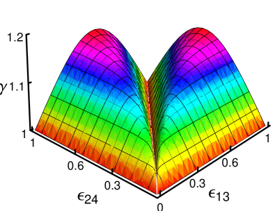
Figure 3: (Color Online) The ratio $\gamma$ between the effective efficiency achievable by squeezing the parameter field and the corresponding quantity obtained by the insertion of a beam splitter as a function of $\epsilon_{13}$ and $\epsilon_{24}$.

As it is apparent from the plot $\gamma$ is symmetric under the exchange of $\epsilon_{13}$ and $\epsilon_{24}$ and achieves its maximum $\gamma\simeq 1.17$ for $\epsilon_{13}=0.5$ and $\epsilon_{24}=1$ or viceversa. The function is not particularly peaked around its maximum and this means that there is a wide range of values for $\epsilon_{13}$ and $\epsilon_{24}$ for which we have a significant gain in squeezing the parameter field in comparison to the insertion of a beam splitter. On the other hand, when one of the two efficiencies is very small then the two methods are equally ineffective. The amount of squeezing needed to achieve CPO strongly depends on the values of the efficiencies. The region of maximum improvement corresponds to a moderate squeezing, i.e. $a$ not too far from one. In Fig. 4 we report the parametric plot of $\gamma$ as a function of the corresponding squeezing: this is a multivalued plot since there are many pairs $(\epsilon_{13},\epsilon_{24})$ for which the same $\gamma$ is achievable, though employing different amounts of squeezing.

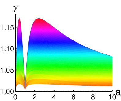
Figure 4: (Color Online) Parametric plot of the ratio $\gamma$ between the effective efficiency achievable by squeezing the parameter field and the corresponding quantity obtained by the insertion of a beam splitter as a function of the squeezing $a$ needed to achieve the compensation.

The two symmetric maxima of Fig. 3 correspond to squeezing parameters which are inverses of each other, ($a\simeq 2.414$ and $a\simeq 0.414$) i.e. they correspond to the same amount of squeezing, but in orthogonal directions. In turn, when the values of the two efficiencies $\epsilon_{13}$ and $\epsilon_{24}$ are close to each other we have

$$a \simeq 1+\frac{\epsilon_{13}-\epsilon_{24}}{\epsilon_{\textrm{m}}^{2}}+\mathcal{O}(\epsilon_{13}-\epsilon_{24})^{2}\,,$$

$$\epsilon_{\textrm{eff}} \simeq\epsilon_{\textrm{m}}+\frac{1}{2}|\epsilon_{13}-\epsilon_{24}|+\mathcal{O}(\epsilon_{13}-\epsilon_{24})^{2}\,,$$

$$\gamma \simeq 1+\frac{|\epsilon_{13}-\epsilon_{24}|}{2\epsilon_{\textrm{m}}}+\mathcal{O}(\epsilon_{13}-\epsilon_{24})^{2}\,.$$

Overall, we conclude that squeezing the parameter field is always convenient, and may lead to a considerable gain in the effective efficiency in comparison to the insertion of a beam splitter. Since the maximum gain corresponds to the use of a moderate amount of squeezing we foresee possible experimental implementations with current technology.

We close this section by comparing the phase distributions obtained by using these two methods of balancing the efficiencies. Suppose, for simplicity, that the signal field is in a coherent state $|z\rangle$ with $z=1$ and the overall efficiencies of the homodyne detectors are $\epsilon_{13}=0.5$ and $\epsilon_{24}=1$. The effective efficiency obtained by using the squeezing method is then $\epsilon_{\textrm{eff}}\simeq 0.828$. We show the phase distributions in Fig. 5 where we have also added the ideal case for comparison. It is clear that the squeezing method provides a distribution which is more peaked around its maximum. To make this more precise, consider the minimum variance of the distribution defined as Lahti3

$$\textrm{Var}_{\textrm{min}}(p)=\inf_{\phi,\varphi\in\mathbb{R}}\,\frac{1}{2\pi}\int_{\varphi-\pi}^{\varphi+\pi}(\phi-\varphi)^{2}p(\phi)\,d\phi$$

Let $p_{\textrm{id}}$, $p_{\textrm{sq}}$ and $p_{\textrm{bs}}$ be the phase distributions obtained with ideal detectors, squeezing, and by using an additional beam splitter. Then the minimum variances are given by

$$\textrm{Var}_{\textrm{min}}(p_{\textrm{id}})\simeq 0.76,$$

$$\textrm{Var}_{\textrm{min}}(p_{\textrm{sq}})\simeq 0.89,$$

$$\textrm{Var}_{\textrm{min}}(p_{\textrm{bs}})\simeq 1.24,$$

which clearly shows the advantage of the squeezing method.

Figure 5: The phase distributions of a coherent state $|z\rangle$ with $z=1$ in the case of ideal detectors (higher dashed line), balancing by squeezing (solid line), and balancing by an additional beam splitter (lower dashed line).

VI Conclusions and outlooks

In this paper we have analyzed in detail the performance of the eight-port homodyne detector as a suitable device to measure covariant phase observables. We have abandoned the traditional assumption of equal quantum efficiencies for the four photodetectors involved in the detection scheme and have investigated in detail the conditions under which the measurement of a CPO may be achieved. We have found that balancing the efficiencies using an additional beam splitter allows to achieve CPO at the price of reducing the overall effective efficiency and we have proved that this CPO is never a smearing of the ideal CPO achievable with unit quantum efficiency. We have also suggested an alternative compensation strategy, where a squeezed vacuum is used as a parameter field, which allows one to increase the overall efficiency in comparison to the passive case using only a moderate amount of squeezing.

In ideal conditions, i.e. for photodetectors with unit quantum efficiencies, the phase-space observables achievable by eight-port homodyning are equivalent to those achievable by six-port homodyning Par97 or heterodyning Yue78 ; Sha84 ; Sha85 . Equivalence also holds in noisy conditions if all the involved photodetectors are assumed to have the same quantum efficiency. In this context a question arises on whether the effects of different quantum efficiencies may result in different phase-space observables or in inequivalent compensation schemes. Work along these lines is in progress and results will be reported elsewhere.

Our results provide a more realistic characterization of phase-space measurements of the optical phase by eight-port homodyning, and are suitable for experimental verification. As a matter of fact, both compensation schemes suggested in this paper may be implemented with current quantum optical technology.

References

- (1) L. Susskind, J. Glogower, Physics 1, 49 (1964).
- (2) P. Carruthers and M. Nieto, Rev. Mod. Phys. 40, 411 (1968).
- (3) R. Lynch, Phys. Rep. 256, 367 (1995).
- (4) R. Tanas, A. Miranowicz, Ts. Gantsog, Progr. Opt. XXXV, 355 (1996).
- (5) D. T. Pegg, S. M. Barnett, J. Mod. Optics 44, 225 (1997).
- (6) V. Peřinová, A. Lukš, J. Peřina, Phase in Optics (World Scientific, Singapore, 1998).
- (7) J.-P. Pellonpää, Covariant Phase Observables in Quantum Mechanics (Ph.D. thesis, University of Turku, 2002). Available at: https://oa.doria.fi/handle/10024/5808
- (8) U. Leonhardt, J. A. Vaccaro, B. Böhmer, H. Paul, Phys. Rev. A 51, 84 (1995).
- (9) M. G. A. Paris, Nuovo Cim. B 111, 1151 (1996); Fizika B 6 63 (1997).
- (10) A. S. Holevo, Sov. Math. (Iz. VUZ) 27, 53 (1983).
- (11) P. Lahti, J.-P. Pellonpää, J. Math. Phys. 40, 4688 (1999).
- (12) N. G. Walker, J. E. Carrol, Opt. Quantum Electr. 18, 355 (1986)
- (13) N. G. Walker, J. Mod. Opt. 34, 16 (1987).
- (14) Y. Lay, H. A. Haus, Quantum Opt. 1, 99 (1989).
- (15) J. W. Noh, A. Fougeres, L. Mandel, Phys. Rev. Lett. 67, 1426 (1991); Phys. Rev. A 45, 424 (1992); Phys. Rev. A 46, 2840 (1992).
- (16) M. Freyberger, K. Vogel, W. P. Schleich, Phys. Lett. A 176, 41 (1993).
- (17) U. Leonhardt, H. Paul, Phys. Rev. 47, 2460 (1993).
- (18) G. M. D’Ariano, M. G. A. Paris, Phys. Rev. A 49, 3022, (1994).
- (19) A. Luis, J. Peřina, Q. Sem. Opt. 8, 873 (1996).
- (20) P. Kochanski, K. Wodkiewicz K. J. Mod. Opt. 44, 2343 (1997).
- (21) J. Rehacek, Z. Hradil, M. Dusek, O. Haderka, M. Hendrych, J. Opt. B 2, 237 (2000).
- (22) M. G. Raymer, J. Cooper, M. Beck, Phys. Rev. A 48, 4617 (1993).
- (23) M. G. A. Paris, A. Chizhov, O. Steuernagel, Opt. Comm. 134, 117 (1997).
- (24) H. P. Yuen and J. H. Shapiro, IEEE Trans. Inf. Theory, 24, 657 (1978); 25, 179 (1979); 26, 78 (1980).
- (25) J. H. Shapiro, S. S. Wagner, IEEE J. Quant. Electron. 20, 803 (1984).
- (26) J. H. Shapiro, IEEE J. Quant. Electron. 21, 237 (1985). Opt. Comm. 134, 117 (1997).
- (27) M. G. A. Paris, G. Landolfi, G. Soliani, J. Phys. A 40, F531 (2007).
- (28) R. H. Hadfield, Nat. Phot. 3, 696 (2009).
- (29) U. Leonhardt, H. Paul, Phys. Rev. A 48, 4598 (1993).
- (30) G. M. D’Ariano, C. Macchiavello, M. G. A. Paris, Phys. Lett. A 198, 286 (1995).
- (31) P. Lahti, J.-P. Pellonpää, J. Schultz, J. Mod. Opt. 57, 1171 (2010).
- (32) A. S. Holevo, Rep. Math. Phys. 16, 385 (1979).
- (33) R. Werner, J. Math. Phys. 25, 1404 (1984).
- (34) J. Kiukas, P. Lahti, J. Mod. Opt. 55, 1891 (2008).
- (35) U. Leonhardt, Measuring the Quantum State of Light (Cambridge University Press, 1997).
- (36) P. Busch, M. Grabowski, P. Lahti, Operational Quantum Physics (Springer-Verlag, 1995).
- (37) P. Lahti, J.-P. Pellonpää, J. Math. Phys. 41, 7352 (2000).
- (38) I. S. Gradshteyn, I. M. Ryzhnik, Table of Integrals, Series, and Products, Corrected and Enlarged Edition (Academic Press, Inc., Orlando, 1980).