Abstract

We present a systematic approach to the linearised Yang-Mills-Higgs equations in the background of a ’t Hooft-Polyakov monopole and use it to unify and extend previous studies of their spectral properties. We show that a quaternionic formulation allows for a compact and efficient treatment of the linearised equations in the BPS limit of vanishing Higgs self-coupling, and use it to study both scattering and bound states. We focus on the sector of vanishing generalised angular momentum and analyse it numerically, putting zero-energy bound states, Coulomb bound states and infinitely many Feshbach resonances into a coherent picture. We also consider the linearised Yang-Mills-Higgs equations with non-vanishing Higgs self-coupling and confirm the occurrence of Feshbach resonances in this situation.

1 Introduction

Solitons - spatially localised and stable solutions of non-linear differential equations - are widely used in modelling physical and biological phenomena. In many of these applications, it is also of interest to study the behaviour of small perturbations around the soliton. In the context of quantum field theory, the small perturbations are interpreted as particles after quantisation [1]. In that case, studying perturbations around a soliton amounts to studying the interaction of these (quantum) particles with the classical soliton. In Skyrme’s model for nuclei [2, 3, 4], for example, the solitons describe nuclei and the small perturbations correspond, after quantisation, to pions. Their properties in the background of a Skyrmion can therefore be interpreted in terms of pion-nucleus scattering.

Mathematically, studying perturbations of a soliton amounts to studying the spectral properties of the linear operator obtained by linearising the soliton equations around the soliton. It turns out that these spectral properties are often interesting, see [1] for a textbook treatment of some examples. A particularly interesting example is provided by magnetic monopoles in $SU(2)$ Yang-Mills-Higgs (YMH) theory. It has long been known that the linearised YMH equations in the background of a monopole have interesting zero-modes in the BPS limit [5, 6, 7] and that they support infinitely many bound states [8]. Scattering of fermions off the monopole has also been studied extensively [9, 10, 11, 12]. However, fairly recently interesting new scattering phenomena were observed. In [13] and, more recently and in more detail in [14], Fodor and Rácz studied spherically symmetric but non-linear perturbations of the ’t Hooft-Polyakov monopole, in the BPS limit. The authors studied the evolution of such excitations numerically and found that the monopole holds on to a significant fraction of the energy from the initial excitation for a surprisingly long time. In particular the amplitude of the excitation decays as $t^{-5/6}$ for late times.

Motivated by this work, Forgács and Volkov carried out a perturbative analysis [15] of the ’t Hooft-Polyakov monopole, still in the BPS limit and preserving the hedgehog form of the monopole. Their linearised equations of motion are a system of two weakly coupled, second order ordinary differential equations. By using the dispersion relation, one of these channels is seen to be massive and one massless. Some intuition about the system is gained by artificially decoupling it and considering only the massive channel. The potential appearing in it has an (attractive) Coulomb tail, so that it possesses infinitely many bound states approaching a critical value, beyond which there is a continuous spectrum. On re-coupling and considering the full system, a phase shift analysis of the massless channel shows that the infinity of bound states in the massive channel turn into an infinity of resonances in the coupled system. The energy held by the resonances leaks out slowly to the massless channel, leading to the long-lived excitation observed by Fodor and Rácz.

The aim of this work is to extend the results of Forgács and Volkov and to place it in the context of other spectral properties of the linearised YMH equations. We develop a quaternionic formalism for studying the linearised YMH equation in the case of vanishing Higgs self-coupling (i.e. in the BPS limit). We show that this quaternionic formalism allows for a systematic treatment of perturbations, organised in terms of the eigenvalues of the generalised angular momentum operator (combining orbital angular momentum, spin and isospin). For vanishing generalised angular momentum we recover the equations studied by Forgács and Volkov but also find another system, consisting of two coupled, second order ordinary differential equations. These have bound states, already found by Bais and Troost in [8]. The two systems found for vanishing generalised angular momentum thus already display a wealth of interesting spectral properties, including bound states at zero energy, bound states embedded in the continuum and resonance scattering. Moreover, the BPS condition allows one to map either of the systems into equivalent but sometimes simpler systems using a first order differential operator (essentially a supersymmetry charge, but we do not consider the fully supersymmetric theory here). This turns out to explain some of the surprising features we find.

We also consider the case of non-vanishing Higgs self-coupling $\lambda$. In this regime, our quaternionic formalism is no longer effective. Thus we do not study general perturbations but instead focus on the generalisation of the system studied by Forgács and Volkov when $\lambda\neq 0$. We find that the Coulomb tail in the massive channel is replaced by an attractive $1/r^{2}$ potential. This is strong enough to support infinitely many bound states after decoupling (by hand), and our numerical analysis suggests that it will also produce infinitely many resonances in the coupled systems. We conclude that the qualitative features found by Forgács and Volkov survive the “switching on” of $\lambda$.

The paper is organised as follows. In Sect. 2, we study the general form of the linearised YMH equation around a background which satisfies the first order BPS equation (which includes the ’t Hooft-Polyakov monopole in the BPS limit). We introduce a quaternionic language and show that the linearised YMH equations for stationary time-dependent perturbations can be expressed as a quaternionic wave equation, supplemented by a background gauge condition. For non-zero kinetic energy there is a second, equivalent form of this wave equation, related to the original one by the application of a Dirac-type operator. Our strategy for studying the linearised YMH equations is therefore to study the quaternionic wave equation and to check if solutions satisfy the background gauge condition.

In Sect. 3, we carry out a partial wave analysis of the quaternionic wave equation and derive two systems of two second order ordinary differential equations which arise in the sector with vanishing generalised angular momentum. We also derive the form of the alternative but equivalent systems obtained by acting with the Dirac-type operator of the previous section. Sect. 4 contains a detailed, numerical investigation of the two systems found in Sect. 3. Even though these systems look superficially very similar, their spectral properties are quite different. One of the systems is the hedgehog system already discussed in [15]; we briefly repeat the analysis of this system, using it to set out our conventions. We then observe that the other system decouples, after application of the Dirac-type operator, into one channel which supports bound states and another which only has scattering states. We are able to relate the bound states to those discussed in [8]. The scattering states do not satisfy the background gauge condition and therefore are not valid bosonic states in the linearised theory, but we point out their relation to the fermionic scattering states studied in [12]. In Sect. 5, we continue our study of $SU(2)$ monopoles, but allow for non-zero Higgs self-coupling. We perturb around the background of the non-BPS ’t Hooft-Polyakov monopole and find scattering resonances in the linearised hedgehog fields. Finally, in Sect. 6 we discuss possible extensions of our work and the interpretation of our results in the context of electric-magnetic duality.

2 Perturbing the BPS Monopole

2.1 The BPS Monopole

Much background material for this section can be found in the textbook [4], to which we refer for details. We work on four-dimensional Minkowski space-time with coordinates $x^{\mu}$, $\mu=0,1,2,3$ and Minkowski metric $\eta_{\mu\nu}=\text{diag}(1,-1,-1,-1)$. We denote the time coordinate by $x^{0}$ or $t$ and write three-component Euclidean vectors with bold letters, e.g. $\mathbf{x}=(x_{1},x_{2},x_{3})$. We write the inner product as $\mathbf{x}\cdot\mathbf{y}$ and $r$ for the spatial radial coordinate, i.e. $r=|\mathbf{x}|=\sqrt{x_{1}^{2}+x_{2}^{2}+x_{3}^{2}}$. The YMH model we are interested in has gauge group $SU(2)$, often referred to as isospin symmetry. Monopoles emerge when the Higgs mechanism breaks the $SU(2)$ symmetry to $U(1)$. In the notation and nomenclature of this paper we treat this $U(1)$ as the gauge group of Maxwell electrodynamics. We work in units where the speed of light and the gauge coupling are 1.

The fields of the YMH model are an $SU(2)$ gauge potential $A_{\mu}$, coupled to a Higgs field $\phi$. Both take values in the Lie algebra $\mathfrak{su(2)}$ and transform in the adjoint representation of $SU(2)$. For the Lie algebra $\mathfrak{su(2)}$, we use the basis ${t_{a}=-\frac{i}{2}\tau_{a}}$, where $\tau_{a},a=1,2,3$, are the Pauli matrices, with brackets $[t_{a},t_{b}]=\epsilon_{abc}t_{c}$, noting that this is not the same convention as [4]. We will also need an inner product $\langle,\rangle$ on $\mathfrak{su(2)}$, which we normalise so that $\langle t_{a},t_{b}\rangle=\delta_{ab}$. The covariant derivative is $D_{\mu}=\partial_{\mu}+[A_{\mu},~{}]$ and the Yang-Mills field strength tensor, or curvature 2-form, is $F_{\mu\nu}=\partial_{\mu}A_{\nu}-\partial_{\nu}A_{\mu}+[A_{\mu},A_{\nu}]$. From this we can extract the non-abelian electric field $E_{i}=F_{0i}$ and the non-abelian magnetic field

$$B_{i}=-\frac{1}{2}\epsilon_{ijk}F_{jk},\quad i,j,k=1,2,3.$$ (2.1)

The YMH Lagrangian density is

$$\mathcal{L}=-\frac{1}{4}\langle F_{\mu\nu}F^{\mu\nu}\rangle+\frac{1}{2}\langle D_{\mu}\phi D^{\mu}\phi\rangle-\frac{\lambda}{4}(1-|\phi|^{2})^{2},$$ (2.2)

where $|\phi|^{2}=\langle\phi,\phi\rangle$. The equations of motion derived from the Lagrangian density are

$$D_{\mu}D^{\mu}\phi =\lambda(1-|\phi|^{2})\phi,$$ (2.3a)

$$D_{\mu}F^{\mu\nu} =[D^{\nu}\phi,\phi].$$ (2.3b)

Static configurations play an important role in this paper as background configurations. For such configurations we work in the temporal gauge $A_{0}=0$, and assume time-independence of the remaining fields $A_{i}$ and $\phi$. Sometimes we collect the static gauge field into a spatial one-form $A=A_{i}dx^{i}$, and write $(A,\phi)$ for the field configuration. For such configurations, the energy computed from the Lagrangian (2.2) can only be finite if we impose the boundary condition

$$|\phi|\rightarrow 1\quad\text{as}\quad r\rightarrow\infty.$$ (2.4)

The equations of motion (2.3) then reduce to

$$D_{i}D_{i}\phi =-\lambda(1-|\phi|^{2})\phi,$$ (2.5a)

$$D_{i}F_{ij} =-[D_{j}\phi,\phi].$$ (2.5b)

The ’t Hooft-Polyakov static monopole solution found in [16, 17] has the hedgehog form

$$A_{i}(\mathbf{x})=\frac{x_{k}}{r^{2}}(1-W(r))\epsilon_{aik}t_{a},\quad\phi(\mathbf{x})=\frac{H(r)}{r^{2}}x_{a}t_{a}.$$ (2.6)

Regularity at the origin requires that $W(0)=1$ and $H(0)=0$, while the boundary conditions at infinity (2.4) are satisfied if we require $H\to-r$ as $r\to\infty$. To recover a more standard definition of the Higgs field $H(r)$ we can scale by $-r$. Our definition of $H(r)$ follows the conventions of Forgács and Volkov in [15] for the hedgehog ansatz, for better comparison with their work.

$H(r)$ and $W(r)$ satisfy differential equations derived from (2.5),

$$\left(-r^{2}\frac{d^{2}}{dr^{2}}+W^{2}+H^{2}-1\right)W =0,$$ (2.7a)

$$\left(-r^{2}\frac{d^{2}}{dr^{2}}+2W^{2}-\lambda(r^{2}-H^{2})\right)H =0.$$ (2.7b)

The BPS limit amounts to setting $\lambda=0$ in (2.2) but maintaining the boundary condition on $\phi$. As the mass of the Higgs is proportional to $\sqrt{\lambda}$, the Higgs field is massless in this limit. The static field equations (2.5) become

$$D_{i}D_{i}\phi =0,$$ (2.8a)

$$D_{i}F_{ij} =-[D_{j}\phi,\phi],$$ (2.8b)

while the equations (2.7) reduce to

$$\left(-r^{2}\frac{d^{2}}{dr^{2}}+W^{2}+H^{2}-1\right)W =0,$$ (2.9a)

$$\left(-r^{2}\frac{d^{2}}{dr^{2}}+2W^{2}\right)H =0.$$ (2.9b)

These equations have an analytic solution found by Prasad and Sommerfield in [18],

$$H(r)=1-r\coth(r),\quad W(r)=\frac{r}{\sinh(r)}.$$ (2.10)

The corresponding field configuration is called the Bogomol’nyi-Prasad-Sommerfield (BPS) monopole.

Further insight into the BPS limit can be gained from considering the static energy

$$E=\frac{1}{2}\int\langle B_{i},B_{i}\rangle+\langle D_{i}\phi,D_{i}\phi\rangle d^{3}x,$$ (2.11)

and rearranging it to

$$E=\frac{1}{2}\int\langle B_{i}+D_{i}\phi,B_{i}+D_{i}\phi\rangle d^{3}x-\int\partial_{i}\langle B_{i},\phi\rangle d^{3}x,$$ (2.12)

where we used the Bianchi identity $D_{i}B_{i}=0$. Using Stokes’ law and the quantisation of magnetic flux, one finds

$$E=\frac{1}{2}\int\langle B_{i}+D_{i}\phi,B_{i}+D_{i}\phi\rangle d^{3}x+2\pi N,$$ (2.13)

where $N$ is an integer called the monopole number. Then for $N>0$ (i.e. monopoles as opposed to anti-monopoles), the energy is bounded by

$$E\geq 2\pi N.$$ (2.14)

This bound is saturated when the Bogomol’nyi equation [19]

$$B_{i}+D_{i}\phi=0$$ (2.15)

holds. The exact monopole solution (2.10) satisfies this equation, and $W(r)$ and $H(r)$ thus satisfy first order equations derived from (2.15), which we will use later:

$$rH^{\prime}(r) =W(r)^{2}+H(r)-1,$$ (2.16a)

$$rW^{\prime}(r) =W(r)H(r).$$ (2.16b)

It is straightforward to check that the first order partial differential equations (2.15) imply the second order equations (2.8), and that the first order ordinary differential equations (2.16) imply the second order equations (2.9).

2.2 Static linearisation

We fix a static background configuration $(A^{s},\phi^{s})$, assumed to satisfy the Bogomol’nyi equation (2.15), write $D^{s}_{i}$ for the covariant derivative $D^{s}_{i}=\partial_{i}+[A^{s}_{i},~{}]$ and likewise $F^{s}_{ij}$ for the curvature of $A^{s}_{i}$. Although we are ultimately interested in time-dependent perturbations, we begin by considering static perturbations $(a,\varphi)$ of $(A^{s},\phi^{s})$ and insert

$$A_{i}=A^{s}_{i}+a_{i},\qquad\phi=\phi^{s}+\varphi,$$ (2.17)

into (2.8). Substituting into (2.8a), applying the static background gauge condition and collecting linear terms in the perturbation we find

$$D_{i}D_{i}\phi\simeq D^{s}_{i}D^{s}_{i}\varphi+[a_{i},D^{s}_{i}\phi^{s}]+D^{s}_{i}[a_{i},\phi^{s}]=0.\\$$ (2.18)

To linearise (2.8b), we need to use that, to linear order,

$$F_{ij}\simeq F^{s}_{ij}+\partial_{i}a_{j}-\partial_{j}a_{i}+[a_{i},A^{s}_{j}]+[A^{s}_{i},a_{j}].$$ (2.19)

Then substituting into (2.8b), the left hand side is

$$D_{i}F_{ij}\simeq D^{s}_{i}F^{s}_{ij}+D^{s}_{i}D^{s}_{i}a_{j}-D^{s}_{i}D^{s}_{j}a_{i}+[a_{i},F^{s}_{ij}].$$ (2.20)

Likewise the right hand side of (2.8b) becomes

$$-[D_{j}\phi,\phi]\simeq[\phi^{s},D^{s}_{j}\phi^{s}]+[\phi^{s},D^{s}_{j}\varphi]+[\varphi,D^{s}_{j}\phi^{s}]+[\phi^{s},[a_{j},\phi^{s}]].$$ (2.21)

Putting (2.20) and (2.21) together and applying the static equation (2.8b) we obtain the linearisation

$$D^{s}_{i}D^{s}_{i}a_{j}-D^{s}_{i}D^{s}_{j}a_{i}+[a_{i},F^{s}_{ij}]\simeq[\phi^{s},D^{s}_{j}\varphi]+[\varphi,D^{s}_{j}\phi^{s}]+[\phi^{s},[a_{j},\phi^{s}]].$$ (2.22)

In most of the remainder of the paper we will only use the covariant derivative $D^{s}_{i}$ and the field strength $F^{s}_{ij}$ associated with a fixed static background configuration. In order to simplify notation we therefore drop the superscripts on $A^{s}_{i},\phi^{s}$, and also on the associated covariant derivative and curvature. In this notation, the linearised Yang Mills Higgs equations for static fields are

$$D_{i}D_{i}\varphi+[a_{i},D_{i}\phi]+D_{i}[a_{i},\phi] =0,$$ (2.23a)

$$D_{i}D_{i}a_{j}-D_{i}D_{j}a_{i}+[a_{i},F_{ij}] =[\phi,D_{j}\varphi]+[\varphi,D_{j}\phi]+[\phi,[a_{j},\phi]].$$ (2.23b)

We can similarly linearise the Bogomol’nyi equations. Substituting (2.17) into the Bogomol’nyi equation (2.15), linearising, using the Bogomol’nyi equation and re-naming $\phi^{s}\rightarrow\phi,A^{s}_{i}\rightarrow A_{i}$ gives

$$\epsilon_{ijk}D_{j}a_{k}=D_{i}\varphi+[a_{i},\phi].$$ (2.24)

There are infinitely many solutions of this equation with $a_{i}=-D_{i}\vartheta$, $\varphi=[\vartheta,\phi]$, where $\vartheta$ is an arbitrary function on $\mathbb{R}^{3}$ with values in $\mathfrak{su(2)}$. These do not physically change the original static solution, as they are infinitesimal gauge transformations. We can exclude such solutions by requiring that perturbations $(a_{i},\varphi)$ satisfy

$$\int\left(\langle a_{i},D_{i}\vartheta\rangle+\langle\varphi,[\vartheta,\phi]\rangle\right)d^{3}x=0,$$ (2.25)

for all $\vartheta$ which are non zero on a closed and bounded subset of $\mathbb{R}^{3}$. The requirement of compact support means that we can integrate by parts and rearrange to obtain the background gauge condition

$$D_{i}a_{i}+[\phi,\varphi]=0.$$ (2.26)

Interestingly, the linearised Bogomol’nyi equations together with the background gauge condition imply the linearised YMH equations (just as solutions of the Bogomol’nyi equation (2.15) are solutions to the static YMH equations (2.8)). To see this, we apply $D_{i}$ to (2.24) and then use (2.15) to obtain (2.23a). In order to derive (2.23b), we apply $D_{j}$ to the background gauge condition (2.26) and $[\phi,\cdot]$ as well as $D_{l}$ to the linearised Bogomol’nyi equation (2.24). The algebra is a little tedious, and makes repeated use of (2.15). We will give a much quicker derivation in the next section.

2.3 Quaternionic Formulation

We will now show that the language of quaternions is very convenient for studying the linearised equations of the previous section. We denote the set of all quaternions as $\mathbb{H}$ and introduce the usual basis $e_{\alpha}$, $\alpha=1,2,3,4$. The real unit quaternion $e_{4}$ commutes with all quaternions and is often written as a $1$ or omitted. The remaining (imaginary) quaternions satisfy

$$e_{i}e_{j}=-\delta_{ij}+\epsilon_{ijk}e_{k}\qquad(i,j,k=1,2,3).$$ (2.27)

We can identify $e_{j}=-i\sigma_{j}$, where $\sigma_{j}$ are again the Pauli matrices (but not denoted $\tau_{i}$ here in order to avoid confusion with the isospin Lie algebra), and $e_{4}$ with the $2\times 2$ identity matrix $\mathbbm{1}_{2}$. The conjugates are

$$\bar{e}_{i}=-e_{i},\quad\bar{e}_{4}=e_{4}.$$ (2.28)

We combine the gauge fields $A_{i}$ and $\phi$ into a quaternion-valued field

$$\mathpzc{Q}=A_{i}e_{i}+\phi.$$ (2.29)

Since $A_{i}$ is an isovector-vector and $\phi$ is an isovector-scalar, we can view this field as a map

$$\mathpzc{Q}:\mathbb{R}^{3}\rightarrow\mathbb{H}\otimes\mathfrak{su}_{2}.$$

Next, we define Dirac-type derivative operators

$$\not{D}=D_{i}e_{i}+[\phi,~{}],\quad\not{D}^{{\dagger}}=D_{i}e_{i}-[\phi,~{}],$$ (2.30)

which act on functions $\mathpzc{q}:\mathbb{R}^{3}\rightarrow\mathbb{H}\otimes\mathfrak{su}_{2}$ by quaternionic multiplication on the quaternions and by commutator on the isospin part $\mathfrak{su}_{2}$. These operators are closely related to the Bogomol’nyi equation for the background field $\mathpzc{Q}$. Note that

$$\not{D}^{\dagger}\not{D}=-D_{i}^{2}-\phi^{2}+(D_{i}\phi-B_{i})e_{i},\quad\not{D}\not{D}^{\dagger}=-D_{i}^{2}-\phi^{2}+(-D_{i}\phi-B_{i})e_{i},$$ (2.31)

so that, for BPS monopoles,

$$\not{D}^{\dagger}\not{D}=-D_{i}^{2}-\phi^{2}+2D_{i}e_{i},\quad\not{D}\not{D}^{\dagger}=-D_{i}^{2}-\phi^{2},$$ (2.32)

by virtue of (2.15).

It turns out that the linearised YMH and BPS equations can both be expressed very compactly in terms of these operators. To see this, let

$$\mathpzc{q}=a_{i}e_{i}+\varphi.$$ (2.33)

We look for the quaternionic expression equivalent to the linearised Bogomol’nyi equation (2.24) and observe that

$$\begin{split}\not{D}\bar{\mathpzc{q}}&=D_{i}a_{i}+[\phi,\varphi]+e_{i}(D_{i}\varphi-\epsilon_{ijk}D_{j}a_{k}-[\phi,a_{i}]).\end{split}$$ (2.34)

The real part of (2.34) vanishing is precisely the background gauge condition (2.26), while setting the complex part to zero is equivalent to (2.24). The linearised Bogomol’nyi equation (2.24) togther with the background gauge condition therefore have the following, very simple quaternionic formulation

$$\not{D}\bar{\mathpzc{q}}=0.$$ (2.35)

This was used extensively in [20].

We now express the linearised YMH equations (2.23) in quaternionic notation, which has not been previously considered. We expect it to be some second order equation in $\not{D}$, since the linearised Bogomol’nyi equation is a first order equation in $\not{D}$. In fact, we will now show that the quaternionic equation

$$\not{D}^{{\dagger}}\not{D}\bar{\mathpzc{q}}=0$$ (2.36)

is equivalent to the linearised field equations (2.23a) and (2.23b), provided the background gauge condition (2.26) holds.

In order to prove our claim we first note a number of useful relations. Using the definition of the curvature as the commutator of covariant derivatives, as well as the Bogomol’nyi equation (2.15) and the definition (2.1) of the non-abelian magnetic field, one finds

$$\epsilon_{lim}D_{l}D_{i}\varphi=\frac{1}{2}\epsilon_{lim}[D_{l},D_{i}]\varphi=\frac{1}{2}\epsilon_{lim}[F_{li},\varphi]=[B_{m},\varphi]=[\varphi,D_{m}\phi].$$ (2.37)

The Leibniz rule, again with the Bogomol’nyi equation (2.15) and the definition (2.1) of the non-abelian magnetic field, gives

$$\epsilon_{lim}D_{l}[\phi,a_{i}]=[F_{im},a_{i}]+\epsilon_{lim}[\phi,D_{l}a_{i}].$$ (2.38)

Then we compute

$$\begin{split}\not{D}^{{\dagger}}\not{D}\bar{\mathpzc{q}}&=\not{D}^{{\dagger}}(D_{i}a_{i}+[\phi,\varphi])+\not{D}^{{\dagger}}e_{i}(D_{i}\varphi-\epsilon_{ijk}D_{j}a_{k}-[\phi,a_{i}])\\ &=\not{D}^{{\dagger}}(D_{i}a_{i}+[\phi,\varphi])\\ &\quad-D_{i}D_{i}\varphi-[a_{i},D_{i}\phi]-D_{i}[a_{i},\phi]\\ &\quad+D_{i}D_{i}a_{j}e_{j}-D_{i}D_{j}a_{i}e_{j}+e_{j}[a_{i},F_{ij}]-e_{j}[\phi,D_{j}\varphi]-e_{j}[\varphi,D_{j}\phi]-e_{j}[\phi,[a_{j},\phi]].\end{split}$$ (2.39)

The terms after the last equality sign are, in the first line, the operator $\not{D}^{{\dagger}}=e_{l}D_{l}-\phi$ applied to the the background gauge expression (2.26), in the second line the linearised field equations (2.23a), and in the third line the linearised field equations (2.23b). Thus, with the background gauge condition $D_{i}a_{i}+[\phi,\varphi]=0$ imposed, the quaternionic equation (2.36) and the linearised static YMH equations (2.23) are equivalent, as claimed.

In the quaternionic notation it is obvious that the first order equation $\not{D}\bar{\mathpzc{q}}=0$ (combining background gauge condition and linearised Bogomol’nyi equation) implies the second order equation $\not{D}^{{\dagger}}\not{D}\bar{\mathpzc{q}}=0$ (and hence the linearised static field equations, since the background gauge is in place).

2.4 Time dependent perturbations

We now introduce time-dependent perturbations around a static configuration $(A^{s}_{i},\phi^{s})$ satisfying (2.15), using the following stationary ansatz

$$A_{i}(t,\mathbf{x})=A_{i}^{s}(\mathbf{x})+a_{i}(\mathbf{x})e^{i\omega t},\qquad\phi(t,\mathbf{x})=\phi^{s}(\mathbf{x})+\varphi(\mathbf{x})e^{i\omega t}.$$ (2.40)

We recall that we work in the temporal gauge $A_{0}=0$ and the BPS limit $\lambda=0$. Inserting the ansatz in the YMH equations (2.3), linearising and re-naming again $\phi^{s}\rightarrow\phi,A^{s}_{i}\rightarrow A_{i}$, we find

$$D_{i}D_{i}\varphi+[a_{i},D_{i}\phi]+D_{i}[a_{i},\phi] =-\omega^{2}\varphi,$$ (2.41a)

$$D_{i}D_{i}a_{j}-D_{i}D_{j}a_{i}+[a_{i},F_{ij}] =[\phi,D_{j}\varphi]+[\varphi,D_{j}\phi]+[\phi,[a_{j},\phi]]-\omega^{2}a_{j}.$$ (2.41b)

For $\omega=0$ we recover the static linearised YMH equation (2.36), as one would expect.

With the results of the previous two subsections, we can express the linearised equations in quaternionic language. Provided the background gauge condition (2.26) holds, the following simple equation

$$\not{D}^{{\dagger}}\not{D}\bar{\mathpzc{q}}=\omega^{2}\bar{\mathpzc{q}}$$ (2.42)

is equivalent to the stationary linearised YMH equations (2.41). This observation is fundamental for the remainder of this paper, and the foundation of our strategy for investigating (2.41) by studying (2.42) and then imposing the background gauge condition.

Like all differential equations, the equation (2.42) can be written as a first order system. In this case, it takes the form of a Dirac equation:

$$\bigg{(}\begin{array}[]{cc}\partial_{t}&\not{D}^{{\dagger}}\\ \not{D}&-\partial_{t}\end{array}\bigg{)}\bigg{(}\begin{array}[]{c}\bar{\mathpzc{q}}\\ \mathpzc{p}\end{array}\bigg{)}=\bigg{(}\begin{array}[]{c}0\\ 0\end{array}\bigg{)},$$ (2.43)

where $\bar{\mathpzc{q}}$ and $\mathpzc{p}$ are quaternion valued fields.

With the stationary ansatz we have the eigenvalue equations

$$\bigg{(}\begin{array}[]{cc}0&\not{D}^{{\dagger}}\\ \not{D}&0\end{array}\bigg{)}\bigg{(}\begin{array}[]{c}\bar{\mathpzc{q}}\\ \mathpzc{p}\end{array}\bigg{)}=\omega\bigg{(}\begin{array}[]{c}\bar{\mathpzc{q}}\\ \mathpzc{p}\end{array}\bigg{)}.$$ (2.44)

This equation is closely related to a Dirac equation studied by Jackiw and Rebbi in [5], where they investigated the zero-energy solutions. Bais and Troost [8] looked at the same Dirac equation, extending the analysis to higher energies, and looking for bound states.

The other second order equation which it is possible to arrange (2.44) into is

$$\not{D}\not{D}^{{\dagger}}\mathpzc{p}=\omega^{2}\mathpzc{p}.$$ (2.45)

This equation is equivalent to (2.42), provided $\omega\neq 0$. The map between solutions is

$$\not{D}\bar{\mathpzc{q}}=\omega\mathpzc{p},\quad\text{and}\quad\not{D}^{\dagger}\mathpzc{p}=\omega\bar{\mathpzc{q}},$$ (2.46)

as seen in (2.44). Explicitly, we can obtain a solution of (2.45) from a solution of (2.42) by applying $\not{D}$ to each side of (2.42) and using (2.46):

$$\not{D}\not{D}^{{\dagger}}\not{D}\bar{\mathpzc{q}}=\omega^{2}\not{D}\bar{\mathpzc{q}}\Rightarrow\not{D}\not{D}^{{\dagger}}\mathpzc{p}=\omega^{2}\mathpzc{p},$$ (2.47)

where we also divided by $\omega$. Conversely, we can also map a solution of (2.45) into a solution of (2.42) by substituting for $\mathpzc{p}$ using (2.46), provided $\omega\neq 0$. As we shall see later in this paper, it is fruitful to investigate both (2.42) and (2.45), using the map (2.46) to relate the results.

Finally, we note that the transformation (2.46) also provides a convenient way of checking if a solution $\bar{\mathpzc{q}}$ of (2.42) satisfies the background gauge condition. According to (2.34), the latter is the requirement that the real part (in the quaternionic sense) of $\not{D}\bar{\mathpzc{q}}$ vanishes. In other words, to see if the background gauge condition holds we simply check if the quaternion $\mathpzc{p}$ obtained from $\bar{\mathpzc{q}}$ according to (2.46) has a vanishing real part.

3 The quaternionic wave equation in the background of the BPS monopole

3.1 Structure and symmetries of the wave equation

We begin our detailed study of the equation (2.42) in the case where the background field is the BPS monopole (2.6), with the profile functions given in (2.10). The Dirac operator introduced in (2.30) now takes the form

$$\not{D}^{\dagger}_{BPS}=(e_{i}\partial_{i})+\frac{(1-W)}{r}(\mathbf{e}\times\hat{\mathbf{x}})\cdot\mathbf{t}-\frac{H}{r}\hat{\mathbf{x}}\cdot\mathbf{t}.$$ (3.1)

Using the equations (2.16) satisfied by the profile functions (2.10) we find

$$\begin{split}D_{i}\phi&=\left(\partial_{i}+\frac{x_{k}}{r^{2}}(1-W)\epsilon_{aik}t_{a}\right)\left(\frac{H}{r^{2}}x_{b}t_{b}\right)\\ &=\delta_{ib}\frac{H}{r^{2}}t_{b}+\frac{x_{i}x_{b}}{r}\left(\frac{H}{r^{2}}\right)^{\prime}t_{b}+(1-W)\left(\frac{H}{r^{2}}\right)\frac{x_{k}x_{b}}{r^{2}}\epsilon_{aik}\epsilon_{abc}t_{c}\\ &=\frac{x_{i}x_{a}}{r^{3}}H^{\prime}t_{a}-\frac{x_{i}x_{a}}{r^{2}}(1+W)\frac{H}{r^{2}}t_{a}+\frac{WH}{r^{2}}t_{i},\end{split}$$ (3.2)

so that

$$\begin{split}(\not{D}^{{\dagger}}\not{D})_{BPS}&=-D_{i}^{2}-\phi^{2}+2D_{i}\phi e_{i}\\ &=-\Delta-\frac{2(1-W)}{r^{2}}\mathbf{L}\cdot\mathbf{t}-\frac{(1-W)^{2}}{r^{2}}\mathbf{t}^{2}+\frac{(1-W)^{2}-H^{2}}{r^{2}}(\hat{\mathbf{x}}\cdot\mathbf{t})^{2}\\ &\qquad+\frac{2H^{\prime}}{r}(\hat{\mathbf{x}}\cdot\mathbf{t})(\hat{\mathbf{x}}\cdot\mathbf{e})-\frac{2(1+W)H}{r^{2}}(\hat{\mathbf{x}}\cdot\mathbf{t})(\hat{\mathbf{x}}\cdot\mathbf{e})+\frac{2WH}{r^{2}}(\mathbf{e}\cdot\mathbf{t}),\end{split}$$ (3.3)

where the orbital angular momentum operator $\mathbf{L}$ has components

$$L_{i}=-\epsilon_{ijk}x_{j}\partial_{k},$$ (3.4)

and the Laplace operator can be written as

$$\Delta=\partial_{1}^{2}+\partial_{2}^{2}+\partial_{3}^{2}=\frac{1}{r}\partial_{r}^{2}r+\frac{1}{r^{2}}\mathbf{L}^{2}.$$ (3.5)

We also note that the differential operator in (2.45) now takes the form

$$\begin{split}(\not{D}\not{D}^{{\dagger}})_{BPS}&=-D_{i}^{2}-\phi^{2}\\ &=-\Delta-\frac{2(1-W)}{r^{2}}\mathbf{L}\cdot\mathbf{t}-\frac{(1-W)^{2}}{r^{2}}\mathbf{t}^{2}+\frac{(1-W)^{2}-H^{2}}{r^{2}}(\hat{\mathbf{x}}\cdot\mathbf{t})^{2}.\end{split}$$ (3.6)

We will use the quaternionic formulation for studying the operators in (3.3) and (3.6). This means that we will let them act on functions

$$q:\mathbb{R}^{3}\rightarrow\mathbb{H}\otimes\mathfrak{su}_{2},$$ (3.7)

as explained after (2.30). We begin with (3.8), which arises directly from the linearisation discussed in the previous section, and look for eigenfunctions, i.e. solutions of

$$(\not{D}^{{\dagger}}\not{D})_{BPS}\bar{q}=\omega^{2}\bar{q}.$$ (3.8)

The BPS monopole is spherically symmetric in the sense that a spatial rotation can be compensated for by an iso-rotation. The operator generating the combined spatial and iso-rotations can be expressed in terms of the angular momentum operator $\mathbf{L}$ (3.4), the spin operator $\mathbf{s}=\frac{1}{2}\mathbf{e}$ (whose components act on the quaternion part of (3.7) via commutator), and the isospin operator $\mathbf{t}$ (whose components $t_{i}=-\frac{i}{2}\tau_{a}$ act in the adjoint representation on the $\mathfrak{su}_{2}$ part of $q$). It is easy to check that, with our conventions, the components of the generalised angular momentum operator

$$\mathbf{J}=\mathbf{L}+\mathbf{s}+\mathbf{t}$$ (3.9)

satisfies $[J_{i},J_{j}]=\epsilon_{ijk}J_{k}$ and commutes with $\not{D}_{BPS}$ and $\not{D}^{{\dagger}}_{BPS}$ defined in (3.1). As a result we are able to organise eigenfunctions of the operator $(\not{D}^{{\dagger}}\not{D})_{BPS}$ in terms of multiplets of the generalised angular momentum operator $\mathbf{J}$. Doing this in practice is the subject of the next section.

3.2 Partial wave analysis

In order to split the set of eigenfunctions in (3.8) into irreducible representations (multiplets) of the generalised angular momentum operator $\mathbf{J}$ we apply basic results from the representation theory of $SU(2)$. Denoting irreducible representations of $SU(2)$ by their spin $j\in\frac{1}{2}\mathbb{N}$ we recall the basic tensor product decomposition rule

$$j_{1}\otimes j_{2}=\bigoplus_{n=|j_{1}-j_{2}|}^{j_{1}+j_{2}}n.$$ (3.10)

From the point of view of representation theory, we may think of quaternions as a direct sum of a spin $0$ and a spin $1$ representation of $\mathbf{s}$:

$$\mathbb{H}_{1}\simeq 0\oplus 1.$$

The quaternionic function (3.7) can be viewed as a tensor product of $(i)$ a scalar function on $\mathbb{R}^{3}$, $(ii)$ a quaternion and, $(iii)$ a spin $1$ representation of the isospin operator $\mathbf{t}$. The three terms in $\mathbf{J}$ act on each of these separately according to $\mathbf{J}=\mathbf{L}\otimes 1\otimes 1+1\otimes\mathbf{s}\otimes 1+1\otimes 1\otimes\mathbf{t}$. If we split the space of scalar functions on $\mathbb{R}^{3}$ further into a tensor product of functions of the radial coordinate $r$ and the space $L^{2}(S^{2})$ of square-integrable functions on the two-sphere, then $\mathbf{J}$ acts trivially on the radial functions, and the decomposition of $L^{2}(S^{2})$ into irreducible representations of the orbital angular momentum operator $\mathbf{L}$ is the usual decomposition of functions on the two-sphere into spherical harmonics:

$$L^{2}(S^{2})=\bigoplus_{l=0}^{\infty}l.$$

Thus, applying the rule (3.10) to the tensor product of quaternions and $\mathfrak{su}_{2}$ we observe

$$(0\oplus 1)\otimes 1=1\oplus 0\oplus 1\oplus 2.$$

Tensoring further with irreducible representations of the orbital angular momentum operator $\mathbf{L}$ we deduce that for $l\geq 2$,

$$l\otimes(0\oplus 1)\otimes 1 =l\otimes(0\oplus 1\oplus 1\oplus 2)$$

$$=l\oplus(l-1)\oplus l\oplus(l+1)\oplus(l-1)\oplus l\oplus(l+1)$$

$$\quad\oplus(l-2)\oplus(l-1)\oplus l\oplus(l+1)\oplus(l+2).$$ (3.11)

For $l=1$ we have

$$1\otimes(0\oplus 1)\otimes 1 =1\otimes(0\oplus 1\oplus 1\oplus 2)$$

$$=1\oplus 0\oplus 1\oplus 2\oplus 0\oplus 1\oplus 2\oplus 1\oplus 2\oplus 3,$$ (3.12)

while for $l=0$ we have

$$0\otimes(0\oplus 1)\otimes 1 =0\oplus 1\oplus 1\oplus 2.$$ (3.13)

We can use these equations to count the number of angular momentum representations that can occur for a given value of the total angular momentum $j$. To do this, we fix a value of $j$ and count, with multiplicity, the values of $l$ which occur on the right hand side of equations (3.2) - (3.13). For $j\geq 2$ we find that $l=j$ contributes four times, $l=j-1$ and $l=j+1$ three times each, and $l=j-2$ and $l=j+2$ once each, giving a total of 12 modes. For $j=1$, the value $l=j+2=3$ does not contribute, and $l=j=2=-1$ is impossible, so only 10 modes occur. Finally, for $j=0$, the possibility $l=0$ occurs once, the possibility $l=1$ twice and $l=2$ once, giving a total of four modes. For a given value of $j$, each of the modes has the usual, additional degeneracy of $2j+1$. However, because of overall invariance of the situation under generalised rotations, these $2j+1$ states are physically equivalent (and obey the same differential equation).

3.3 The $j=0$ sector

The four modes with $j=0$ can be constructed very simply by combining $l=0,1,2$ functions with the quaternionic and isospin degrees of freedom to obtain overall scalars under the action of $\mathbf{J}$. Since all states must have isospin 1, the $l=0$ (constant) function can only be combined with $\mathbf{e}\cdot\mathbf{t}$ to obtain an overall scalar. Using the cartesian coordinates of the unit vector $\hat{\mathbf{x}}$ on the spatial two-sphere as the three $l=1$ states, we can obtain one overall scalar from the scalar ($s=0$) field as $\hat{\mathbf{x}}\cdot\mathbf{t}$. Another overall scalar can be constructed from the vector $(s=1)$ field as $\hat{\mathbf{x}}\cdot(\mathbf{e}\times\mathbf{t})$. Finally, the five independent functions spanning the $l=2$ multiplet are the components of the tensor $\hat{x}_{i}\hat{x}_{j}-\frac{1}{3}\delta_{ij}$. We can combine these with the isovector and the spin $1$ part of the quaternion as $(\hat{\mathbf{x}}\cdot\mathbf{t})(\hat{\mathbf{x}}\cdot\mathbf{e})-\frac{1}{3}\mathbf{e}\cdot\mathbf{t}$ to obtain an overall scalar. We thus have four basis states of the $j=0$ sector, and can use any linear combination (with coefficients being functions of $r$) to study the $j=0$ sector of (3.8). It turns out that, for our purposes, the following basis states are most convenient:

$$v_{1} =(\hat{\mathbf{x}}\!\cdot\!\mathbf{t})(\hat{\mathbf{x}}\!\cdot\!\mathbf{e})-\mathbf{e}\!\cdot\!\mathbf{t}$$ (3.14a)

$$v_{2} =(\hat{\mathbf{x}}\!\cdot\!\mathbf{t})(\hat{\mathbf{x}}\!\cdot\!\mathbf{e})$$ (3.14b)

$$v_{3} =\hat{\mathbf{x}}\!\cdot\!(\mathbf{e}\times\mathbf{t})$$ (3.14c)

$$v_{4} =\hat{\mathbf{x}}\!\cdot\!\mathbf{t}.$$ (3.14d)

We note that $v_{3}$ and $v_{4}$ are perturbations of the hedgehog fields as defined in (2.6) and are the assumed shape of the perturbations used in [15].

It is worth interpreting our chosen basis physically before proceeding with the mathematical analysis. The generator $\hat{\mathbf{x}}\!\cdot\!\mathbf{t}$ in the isospin Lie algebra is in the direction of the asymptotic Higgs field and thus the generator of the unbroken $U(1)$ subgroup of the original isospin symmetry. Even though the YMH model studied here is not a realistic physical model, we adopt a terminology where this $U(1)$ is interpreted as the gauge group of electromagnetism. Then we note that $v_{2}$ is the unbroken part of the $\mathfrak{su}_{2}$ gauge field and can therefore be thought of as the photon field. The other spin $1$ states $v_{1}$ and $v_{3}$ are eigenstates of $(\hat{\mathbf{x}}\!\cdot\!\mathbf{t})^{2}$ with eigenvalue $-1$ and therefore have electric charge $\pm 1$. Neither of them is an eigenstate of $\hat{\mathbf{x}}\!\cdot\!\mathbf{t}$ so both should be thought of as linear combinations of excitations of the charged $W$-bosons in this model. Finally, the spin zero state $v_{4}$ is proportional to the asymptotic value of Higgs field and describes a massless and uncharged excitations of the Higgs field. We still need to ascertain which linear combination of these states satisfies the background gauge condition (2.26). We will do this below by applying the operator $\not{D}$, as outlined at the end of Sect. 2.4.

Our next task is the application of the operator $(\not{D}^{{\dagger}}\not{D})_{BPS}$ (3.3) to a linear combination

$$\bar{\mathpzc{q}}=\sum_{n=1}^{4}b_{n}(r)v_{n},$$ (3.15)

of the basis functions of the $j=0$ sector. In order to organise the calculation we note that $(\not{D}^{{\dagger}}\not{D})_{BPS}$ is a linear combination of the operators $\Delta$, $\mathbf{L}\cdot\mathbf{t}$, $\mathbf{t}^{2}$, $(\hat{\mathbf{x}}\cdot\mathbf{t})^{2}$, $(\hat{\mathbf{x}}\cdot\mathbf{e})(\hat{\mathbf{x}}\cdot\mathbf{t})$ and $\mathbf{e}\cdot\mathbf{t}$, multiplied by simple functions of $W$ and $H$. We list, in Table 1, the action of the relevant operators on the modes $v_{1},\ldots,v_{4}$ (3.14).

Table 1: The action of the operators in (3.3) on each of the zero angular momentum modes (3.14).

	$v_{1}$	$v_{2}$	$v_{3}$	$v_{4}$
$\mathbf{L}^{2}$	$-2(v_{1}+2v_{2})$	$-2(v_{1}+2v_{2})$	$-2v_{3}$	$-2v_{4}$
$\mathbf{L}\cdot\mathbf{t}$	$v_{1}+2v_{2}$	$v_{1}+2v_{2}$	$v_{3}$	$2v_{4}$
$\mathbf{t}^{2}$	$-2v_{1}$	$-2v_{2}$	$-2v_{3}$	$-2v_{4}$
$(\hat{\mathbf{x}}\cdot\mathbf{t})^{2}$	$-v_{1}$	$0$	$-v_{3}$	$0$
$(\hat{\mathbf{x}}\cdot\mathbf{e})(\hat{\mathbf{x}}\cdot\mathbf{t})$	$v_{1}$	$0$	$v_{3}$	$0$
$\mathbf{e}\cdot\mathbf{t}$	$v_{1}-2v_{2}$	$-v_{1}$	$v_{3}-2v_{4}$	$-v_{3}$

Using (1), we find that (3.8) becomes

$$\begin{split}&\Big{(}-r(rb_{1})^{\prime\prime}v_{1}-r(rb_{2})^{\prime\prime}v_{2}-r(rb_{3})^{\prime\prime}v_{3}-r(rb_{4})^{\prime\prime}v_{4}\Big{)}+\Big{(}2b_{1}v_{1}+2b_{2}v_{1}+4b_{1}v_{2}\\ &\quad+4b_{2}v_{2}+2b_{3}v_{3}+2b_{4}v_{4}\Big{)}+\Big{(}-2(1-W)b_{1}v_{1}-2(1-W)b_{2}v_{1}\\ &\quad-4(1-W)b_{1}v_{2}-4(1-W)b_{2}v_{2}-2(1-W)b_{3}v_{3}-4(1-W)b_{4}v_{4}\Big{)}\\ &\quad+\Big{(}2(1-W)^{2}b_{1}v_{1}+2(1-W)^{2}b_{2}v_{2}+2(1-W)^{2}b_{3}v_{3}+2(1-W)^{2}b_{4}v_{4}\Big{)}\\ &\quad+\Big{(}(-(1-W)^{2}+H^{2})b_{1}v_{1}+(-(1-W)^{2}+H^{2})b_{3}v_{3}\Big{)}\\ &\quad+\Big{(}2(rH^{\prime}-(1+W)H)b_{1}v_{1}+2(rH^{\prime}-(1+W)H)b_{3}v_{3}\Big{)}+\Big{(}2WHb_{1}v_{1}\\ &\quad-2WHb_{2}v_{1}-4WHb_{1}v_{2}+2WHb_{3}v_{3}-2WHb_{4}v_{3}-4WHb_{3}v_{4}\Big{)}\\ &=r^{2}\omega^{2}(b_{1}v_{1}+b_{2}v_{2}+b_{3}v_{3}+b_{4}v_{4}).\end{split}$$ (3.16)

Each group of terms which is bracketed in (3.16) comes from one part of (3.8). We compare coefficients of $v_{1},v_{2},v_{3}$ and $v_{4}$ in (3.16) to obtain equations for the radial functions $b_{n}(r)$. We find that $b_{1}(r)$ and $b_{2}(r)$ are coupled and that $b_{3}(r)$ and $b_{4}(r)$ are coupled. As noted previously, $b_{3}(r)$ and $b_{4}(r)$ are related to the functions $w(r)$ and $h(r)$ in [15], as they are also perturbations of the basic hedgehog fields (2.10). The coupling is not quite symmetric but this can be remedied by defining

$$w=rb_{3},\quad h=\frac{rb_{4}}{\sqrt{2}}.$$ (3.17)

A similar redefinition

$$v=rb_{1},\quad\alpha=\frac{rb_{2}}{\sqrt{2}},$$ (3.18)

for the other coupled system aids comparison with the previous work, and again results in the coupling being symmetric.

With these abbreviations, we conclude that the insertion of

$$\bar{\mathpzc{q}}=\frac{1}{r}(vv_{1}+\sqrt{2}\alpha v_{2}+wv_{3}+\sqrt{2}hv_{4}),$$ (3.19)

into (3.8) gives a system of second order differential equations which decouples into two systems:

$$\left(-\frac{d^{2}}{dr^{2}}+\frac{3W^{2}+H^{2}-1}{r^{2}}\right)v-\frac{2\sqrt{2}W(H-1)}{r^{2}}\alpha =\omega^{2}v,$$ (3.20a)

$$\left(-\frac{d^{2}}{dr^{2}}+\frac{2W^{2}+2}{r^{2}}\right)\alpha-\frac{2\sqrt{2}W(H-1)}{r^{2}}v =\omega^{2}\alpha,$$ (3.20b)

and

$$\left(-\frac{d^{2}}{dr^{2}}+\frac{3W^{2}+H^{2}-1}{r^{2}}\right)w-\frac{2\sqrt{2}WH}{r^{2}}h =\omega^{2}w,$$ (3.21a)

$$\left(-\frac{d^{2}}{dr^{2}}+\frac{2W^{2}}{r^{2}}\right)h-\frac{2\sqrt{2}WH}{r^{2}}w =\omega^{2}h.$$ (3.21b)

As noted, $w(r)$ and $h(r)$ are perturbations of the hedgehog fields $W(r)$ and $H(r)$, and thus we could have obtained (3.21) by linearising (2.16). This is what is done in [15]. In the following sections we will investigate bound and scattering states in the systems (3.20) and (3.21). Recalling the interpretation of the basis (3.14) we note that the system (3.20) describes a photon mode interacting with a $W$-boson mode, and that (3.21) describes a massless Higgs perturbation interacting with a $W$-boson mode. Correspondingly, we will often refer to the former as the photon system and the latter as the Higgs system.

So far, we have focussed on the equation (2.42) since it is directly related to the linearised YMH equations. The alternative but equivalent equation (2.45), however, also plays an important role in our analysis. As explained at the end of Sect. 2.4, the background gauge condition 2.26 is conveniently implemented in this formulation. It also turns out that the equation(2.45) is also sometimes easier to analyse than (2.42).

Recalling the definition (3.6), we thus consider the eigenvalue problem

$$(\not{D}\not{D}^{{\dagger}})_{BPS}\mathpzc{p}=\omega^{2}\mathpzc{p}.$$ (3.22)

Inserting, in analogy to (3.19), the expression

$$\mathpzc{p}=\frac{1}{r}(\chi v_{1}+\sqrt{2}\psi v_{2}+\xi v_{3}+\sqrt{2}\zeta v_{4}),$$ (3.23)

for four radial functions $\xi,\eta,\chi,\psi$ we obtain again two systems of second order differential equations:

$$\left(-\frac{d^{2}}{dr^{2}}+\frac{W^{2}+H^{2}+1}{r^{2}}\right)\xi =\omega^{2}\xi,$$ (3.24a)

$$\left(-\frac{d^{2}}{dr^{2}}+\frac{2W^{2}}{r^{2}}\right)\zeta =\omega^{2}\zeta,$$ (3.24b)

and

$$\left(-\frac{d^{2}}{dr^{2}}+\frac{W^{2}+H^{2}+1}{r^{2}}\right)\chi+\frac{2\sqrt{2}W}{r^{2}}\psi =\omega^{2}\chi,$$ (3.25a)

$$\left(-\frac{d^{2}}{dr^{2}}+\frac{2W^{2}+2}{r^{2}}\right)\psi+\frac{2\sqrt{2}W}{r^{2}}\chi =\omega^{2}\psi.$$ (3.25b)

According to (2.46), we can relate a solution (3.19) of (3.8) to a solution (3.23) of (3.22) via the Dirac operator $\not{D}^{\dagger}_{BPS}$ in (3.1) according to

$$\omega\bar{\mathpzc{q}}=\not{D}^{\dagger}_{BPS}\mathpzc{p}.$$ (3.26)

We are now in a position to apply the background gauge condition (2.26) to solutions of (2.45). As discussed at the end of Sect. 2.4, we can do this by ensuring that the quaternion $\mathpzc{p}$ has no real quaternionic part. Of all the basis elements (3.14), only $v_{4}$ is real in the quaternionic sense. Hence solutions of the form (3.23) correspond, via (3.26), to solutions of the linearised YMH equations if the coefficient function $\zeta$ in (3.23) is identically zero. Note that, according to (3.24), this can be imposed consistently since $\zeta$ satisfies a homogeneous linear equation and does not couple to any other mode.

Working out the relation (3.26) explicitly is a little tedious, but can be done by careful application of some of the results in (1) as well as the application of the operator $(e_{i}\partial_{i})$ to $v_{1},\ldots,v_{4}$. It can be seen without too much effort that the transformation (3.26) permutes the basis elements $v_{1},\ldots,v_{4}$. In particular, the coefficient functions $\xi,\zeta$ of $v_{3},v_{4}$ are mapped to the coefficient functions $v,\alpha$ of $v_{1},v_{2}$. Equally, the coefficient functions $\chi,\psi$ of $v_{1},v_{2}$ are mapped to the coefficient functions $w,h$ of $v_{3},v_{4}$. Since the background gauge condition does not restrict the functions $\chi$ and $\psi$, we deduce that any solution of (3.21) satisfies the background gauge condition.

However, in order to understand the implication of the background gauge for (3.20), we need to know the relation between $\xi,\zeta$ and $v,\alpha$. To compute the effect of applying (3.1) to the basis (3.14) we note that, in terms of the usual spherical coordinates $(r,\theta,\varphi)$ for $\mathbb{R}^{3}$,

$$\hat{\mathbf{x}}=\begin{pmatrix}\sin\theta\cos\varphi\\ \sin\theta\sin\varphi\\ \cos\theta\end{pmatrix},\qquad\hat{\mathbf{\theta}}=\partial_{\theta}\hat{\mathbf{x}}=\begin{pmatrix}\cos\theta\cos\varphi\\ \cos\theta\sin\varphi\\ -\sin\theta\end{pmatrix},\qquad\hat{\mathbf{\varphi}}=\partial_{\varphi}\hat{\mathbf{x}}=\begin{pmatrix}-\sin\varphi\\ \phantom{-}\cos\varphi\\ 0\end{pmatrix},\qquad$$

and

$$\hat{\mathbf{x}}\times\mathbf{L}=\hat{\mathbf{\theta}}\partial_{\theta}+\frac{\hat{\mathbf{\varphi}}}{\sin\theta}\partial_{\varphi}.$$

Therefore

$$e_{i}\partial_{i}=\hat{\mathbf{x}}\!\cdot\!\mathbf{e}\,\partial_{r}+\frac{1}{r}\hat{\mathbf{\theta}}\!\cdot\!\mathbf{e}\,\partial_{\theta}+\frac{1}{r\sin\theta}\hat{\mathbf{\varphi}}\!\cdot\!\mathbf{e}\,\partial_{\varphi}=\hat{\mathbf{x}}\!\cdot\!\mathbf{e}\,\partial_{r}+\frac{1}{r}\mathbf{e}\!\cdot\!\hat{\mathbf{x}}\times\mathbf{L}.$$

Then we compute, for example,

$$(e_{i}\partial_{i})\,v_{4}=-\frac{1}{r}v_{1},\quad(e_{i}\partial_{i})\,v_{3}=\frac{1}{r}(2v_{2}-v_{1}).$$

Evaluating the other terms (3.26) we arrive at

$$\omega\alpha =\frac{d\zeta}{dr}-\frac{\zeta}{r}+\frac{\sqrt{2}W}{r}\,\xi,$$ (3.27a)

$$\omega v =-\frac{d\xi}{dr}-\frac{H}{r}\,\xi-\frac{\sqrt{2}W}{r}\zeta.$$ (3.27b)

Remarkably, the transformation (3.27) relates the coupled system (3.20) to the decoupled system (3.24). Thus, the most efficient way of studying the the coupled system (3.20) is to look at (3.24) instead, and then apply (3.27). In addition, if one is only interested in bosonic modes satisfying the background gauge condition (as we are in this paper), one should set $\zeta$ to zero.

4 Spectral properties of the $j=0$ sector

4.1 General considerations

Before we turn to the numerical investigation of bound states and scattering in the $j=0$ sector, we note some general features of the systems (3.20) and (3.21) on the one hand and (3.24) and (3.25) on the other. For this purpose we note the asymptotic behaviour of the coefficient functions $W$ and $H$ (2.10):

$$W(r)\approx 1-\frac{r^{2}}{6},\quad H(r)\approx-\frac{r^{2}}{3}\quad\text{for small}\,r,$$ (4.1)

and

$$W(r)\approx\frac{r}{2}e^{-r},\quad H(r)\approx 1-r+O(e^{-r})\quad\text{for large}\,r.$$ (4.2)

It follows that the systems (3.20) and (3.21) both decouple at large values of $r$. We can think of them as two channels which are coupled in the region of the background monopole but whose coupling falls off exponentially fast as we go away from the core of the monopole. It is instructive to set the coupling terms to zero and consider the resulting single channels. The equations (3.20a) for $v$ and (3.21a) for $w$ are the same after decoupling, and take the form

$$\left(-\frac{d^{2}}{dr^{2}}+\frac{3W^{2}+H^{2}-1}{r^{2}}\right)v=\omega^{2}v.$$ (4.3)

The potential appearing in this equation has the asymptotic form

$$\frac{3W^{2}+H^{2}-1}{r^{2}}\approx 1-\frac{2}{r}+O(e^{-r})\quad\text{as}\;r\rightarrow\infty,$$ (4.4)

and, in particular, tends to the positive constant $1$ for large $r$. Thus, thinking of (4.3) as the spatial part of a radial wave equation, we see that its wave solutions correspond to massive particles of mass $1$, which is in agreement with our interpretation of $v$ and $w$ as excitations of the $W$-bosons in YMH theory. By contrast, the equation for the function $\alpha$ after decoupling contains the potential

$$\frac{2W^{2}+2}{r^{2}}\approx\frac{2}{r^{2}}+O(e^{-r})\quad\text{for large}\,r,$$ (4.5)

while the equation for the function $h$ after decoupling contains the potential

$$\frac{2W^{2}}{r^{2}}\approx O(e^{-r})\quad\text{for large}\,r.$$ (4.6)

Therefore, the corresponding radial waves are massless excitations, in agreement with their interpretation as, respectively, photon and Higgs excitations.

The potential $(3W^{2}+H^{2}-1)/r^{2}$ is plotted in Fig. 1. The plot and the appearance of the attractive Coulomb tail in the asymptotic form (4.4) suggest that the Sturm-Liouville problem (4.3) should have an infinity of bound states for $\omega^{2}<1$ accumulating at $\omega^{2}=1$, with a continuous spectrum for $\omega^{2}>1$.

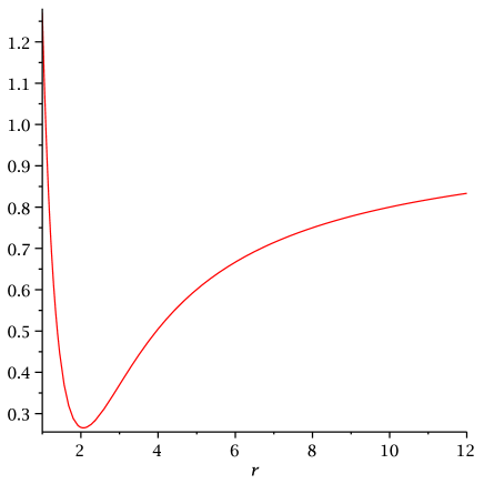
Figure 1: The potential $\frac{3W^{2}+H^{2}-1}{r^{2}}$ plotted against $r$.

The coupling of massless channels to a massive channel with infinitely many bound states constitutes the generic situation for the occurrence of Feshbach resonances, or quasi-normal modes. We give a brief summary and references in Appendix A. On the grounds of the general theory, we might expect both (3.20) and (3.21) to exhibit resonance scattering for $0<\omega^{2}<1$. However, we also note an important difference between the systems (3.20) and (3.21). It follows from (4.1) that the coupling terms in (3.20) are singular at $r=0$, whereas they are smooth for (3.21).

Turning now to the systems (3.24) and (3.25) we observe they, too, consist of a massive and a massless channel each. The potential in the massive channels is

$$\frac{W^{2}+H^{2}+1}{r^{2}}\approx 1-\frac{2}{r}+\frac{2}{r^{2}}+O(e^{-r})\quad\text{as}\;r\to\infty,$$ (4.7)

and, because of the attractive Coulomb term, should again support infinitely many bound states. However, while the system (3.25) has the same generic form as the photon and Higgs systems (3.20) and (3.21) discussed above, the equations in (3.24) are decoupled. As a result, we expect this system to have true bound states for the excitation denoted $\xi$ in the range $0<\omega^{2}<1$. There are scattering states in the excitation $\zeta$, but these do not satisfy the background gauge condition, as already discussed after (3.26). Hence, on the basis of the decoupled form (3.24), we expect the system (3.20) to have infinitely many bound states and no (physical) scattering states in the range $0<\omega^{2}<1$. This is in marked contrast with the Feshbach resonances of the Higgs system (3.21).

Before we present our numerical results we briefly comment on or numerical methods. All of our scattering calculations require a shooting-to-a-fitting-point method for finding solutions which decay at large enough values in one of the channels. Numerical instability would always create difficulties where the exponentially increasing term creeps into the solution. Thus, we choose an appropriately large value of $r$ to integrate to and use a shooting method to find the decaying solution.

4.2 Bound states

It is well known that the zero-modes of the ’t Hooft-Polyakov monopole give rise to zero-energy bound states of the linearised YMH equations. The zero-modes of the ’t Hooft-Polyakov monopole are obtained from infinitesimal translations in $\mathbb{R}^{3}$ and a special ‘large’ gauge transformation generated by the Higgs field itself. This transformation does not vanish at infinity and is therefore considered as a physical symmetry transformation rather than a gauge transformation. The infinitesimal form of the ‘large gauge transformation’ generated by the Higgs field is

$$\delta\phi=0,\quad\delta A_{i}=D_{i}\phi=-B_{i}.$$ (4.8)

In our quaternionic formulation the corresponding zero-mode is simply

$$\mathpzc{q}_{\phi}=e_{i}B_{i},$$ (4.9)

while the other three zero-modes related to translations are

$$\mathpzc{q}_{k}=e_{k}(e_{i}B_{i}).$$ (4.10)

It is easy to check that (4.9) (and hence (4.10)) satisfy the linearised Bogomol’nyi equation (2.35), and hence (3.8) for $\omega=0$. Of the four zero-modes just found, only $\mathpzc{q}_{\phi}$ has $j=0$. It has the explicit form

$$B_{i}=-D_{i}\phi=-\frac{x_{i}x_{a}}{r^{3}}H^{\prime}t_{a}+\frac{x_{i}x_{a}}{r^{2}}(1+W)\frac{H}{r^{2}}t_{a}-\frac{WH}{r^{2}}t_{i},$$ (4.11)

and is thus a linear combination of the basis states $v_{1}$ and $v_{2}$ as defined in (3.14). In particular, it is therefore a solution of the photon system (3.21).

Bais and Troost first investigated bound states in single channels arising in the linearised BPS system in [8]. In particular, they computed bound state energies in the system (3.24a). For completeness of our discussion we have repeated the numerical analysis here. Using the NAG shooting method D02KEF for Sturm-Liouville type problems we find the eigenvalues $\omega^{2}_{n}$ and hence $\omega_{n}>0$ of the first few bound states of (3.24a), to 3 significant figures. As explained in our qualitative discussion in the previous section, we expect there to be infinitely many Coulomb bound states in this channel. We can estimate their energies by neglecting the exponentially small terms in the potential (4.7) and using the standard formula for Coulomb bound state energies. In Table 2 we list both the numerically computed bound state energies of (3.24a) and the Coulomb approximations

$$\Omega_{n}=\sqrt{1-\frac{1}{(n+1)^{2}}},$$ (4.12)

where we used the standard expression for Coulomb bound state energies, recalling that $l=1$ in this case by virtue of the $1/r^{2}$-term in (4.7). Even for very small $n$, the Coulomb approximation is surprisingly good.

$$\begin{array}[]{ccccccc}\hline\cr\hline\cr n&1&2&3&4&11\\ \hline\cr\omega_{n}&0.877&0.946&0.970&0.980&0.997\\ \Omega_{n}&0.866&0.943&0.968&0.980&0.996\\ \hline\cr\hline\cr\end{array}$$

Table 2: Values for $\omega_{n}$ for the eigenvalue problem (3.24a), and $\Omega_{n}$ given in (4.12)

We have also computed the wavefunctions $\xi_{n}$, $n=1,2,\ldots$ for each of the bound states. They have the standard form of Coulomb bound states, but it is interesting to note that they correspond, via (3.27), to bound states in the coupled system (3.20). The functions $v$ and $\alpha$ for each of the bound states describe, via (3.19), the profile of the excited monopole. Since $h$ and $w$ both vanish for this excitation the bound state only involves the photon excitation $\alpha$ and the component $v$ of the field describing the W-boson.

From the point of view of the system (3.20), it is surprising that there are true bound states. As explained in Sect. 4.1, one would generically expect two-channel problems like (3.20) to have Feshbach resonances, but no bound states.

4.3 Scattering

In Appendix A we discuss what kind of coupled systems are likely to possess Feshbach resonances. Both (3.20) and (3.21) have the required features in the parameter range $0<\omega^{2}<1$: they consist of two channels which are weakly coupled at large distances, and are such that, after removing the coupling term, there are bound states in one channel and only scattering states in the other. In fact, the system (3.21) shows exactly the expected Feshbach resonance behaviour. This was first noticed by Forgács and Volkov in [15], and we will revisit it below. However, we will also see that the system (3.20), whose bound states we analysed in the previous section, has no scattering states which satisfy the background gauge condition.

We begin with a brief review of the results of [15]. This will establish our conventions and terminology and serve as a preparation of our generalisation in Sect. 5. The system (3.21) has a regular singular point at the origin, which means that the numerical integration must start a little away from $r=0$. We make a series expansion near $r=0$ and find the following leading terms

$$w\approx Ar^{2},\qquad h\approx Br^{2}\quad\text{for small}\;r,$$ (4.13)

with real constants $A,B$. Because of the linearity of the problem we can scale the solution to fix one of those constants. The remaining free constant plays the role of the shooting parameter.

Once the correct initial conditions are determined to ensure a decaying solution $w$ (for $\omega^{2}<1$), we can consider the scattering problems in the massless channel (3.21b). It has the general form

$$\left(-\frac{d^{2}}{dr^{2}}+\frac{l(l+1)}{r^{2}}+V(r)-\omega^{2}\right)u(r)=0,$$ (4.14)

where $V(r)\to 0$ as $r\to\infty$ exponentially fast. In the equation for $h$, the total potential is (4.6) so $l=0$.

For large values of $r$, where $V$ can be neglected, the solution must be a combination of spherical Bessel functions

$$u(r)=r\left(A_{l}j_{l}(\omega r)+B_{l}y_{l}(\omega r)\right),\quad\text{for}\quad r\;\text{large}.$$ (4.15)

Since, asymptotically, $j_{l}(\omega r)\approx\sin(\omega r-\frac{l}{2}\pi)/(\omega r)$ and $y_{l}(\omega r)\approx-\cos(\omega r-\frac{l}{2}\pi)/(\omega r)$ we have the asymptotic form

$$u(r)\approx\frac{\sqrt{A_{l}^{2}+B_{l}^{2}}}{\omega^{2}}\sin(\omega r+\delta_{l}-\frac{l}{2}\pi)$$

of the radial wavefunction, with the phase shift defined via

$$\tan({\delta_{l}})=-\frac{B_{l}}{A_{l}}.$$

By evaluating both sides of (4.15) for two large values of $r$ (or by evaluating both sides and their derivatives for large $r$) we extract the coefficients $A_{l}$ and $B_{l}$, for each value of $\omega$ , and hence the phase shift $\delta_{l}$ at $\omega$. The latter determines the partial scattering cross section according to the standard expression

$$\sigma_{l}(\omega)=\frac{4\pi(2l+1)}{\omega^{2}}\sin^{2}\delta_{l}(\omega),$$

and the total cross section according to

$$\sigma(\omega)=\frac{4\pi}{\omega^{2}}\sum\limits_{l=0}^{\infty}(2l+1)\sin^{2}\delta_{l}(\omega).$$

Near a resonance, $\delta_{l}$ increases rapidly by $\pi$. The function $\sin^{2}\delta_{l}(\omega)$ takes values between $0$ and $1$, is maximal at the resonance and is thus an expedient quantity to plot when looking for resonances.

Applying this procedure to the $l=0$ contribution to the scattering cross section for the massless channel $h$ from the Higgs system (3.21) we confirm the result shown in Fig.1 of [15], suggesting infinitely many resonances as the energy approaches the critical value $\omega^{2}=1$. A graph of $\sin^{2}\delta(\omega)$ against $\omega$ for the massless channel $h$ is shown in Fig. 2.

We have also computed the bound state energies of the decoupled massive channel (4.3) which occurs in both (3.20) and (3.21), using the numerical method summarised in the previous section. They were also computed in [15]. Our results are listed in Table 3, given to 4 significant figures. They are in good agreement with the results in Table II of [15]. Comparing with Fig. 2, one sees that the energies of the bound states are close to the energy values where the resonances occur. The bound states of the decoupled problem have turned into resonances in the coupled problem. This is typical Feshbach behaviour.

$n$	1	2	3	4	5	10	15
$\omega_{n}$	0.7984	0.9263	0.9618	0.9766	0.9842	0.9956	0.9980

Table 3: Values of $\omega_{n}$ for the eigenvalue problem (4.3).

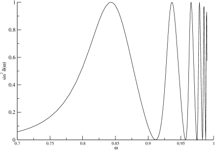
Figure 2: For the system (3.21), the partial scattering cross section $\sin^{2}\delta_{0}(\omega)$ is plotted against $\omega$.

Next we turn to scattering states in the system (3.20), exploiting the equivalence with the simpler system (3.24). In the energy range that we are interested in, with $\omega^{2}<1$, only the equation (3.24b) has scattering solutions. However, from our discussion after (3.26) we know that a non-vanishing $\zeta$ violates the background gauge condition. We can therefore conclude that the system (3.20) has no scattering states satisfying the background gauge condition in the range $\omega^{2}<1$. This is surprising in view of the superficial similarity to the system (3.21), which, as we saw above, shows interesting resonance scattering.

We end this section with some observations about scattering solutions of (3.24b). Even though they do not satisfy the background gauge condition and therefore do not correspond to solutions of the linearised YMH equations we expect them to play a role in the supersymmetric version of the theory as fermonic scattering states. The scattering problem associated to (3.24b) is also of independent interest since it can be solved exactly. Inserting the expression (2.10) for the profile function $W$, the equation (3.24b) takes the following simple form:

$$-\frac{d^{2}\zeta}{dr^{2}}+\frac{2}{\sinh^{2}(r)}\zeta=\omega^{2}\zeta.$$ (4.16)

This equation was studied in the context of fermion scattering off monopoles in [12] (the authors there did not include the Higgs field, but this does enter (4.16) anyway). A scattering solution regular at the origin is

$$\zeta(r)=(i\omega+\coth(r))e^{-i\omega r}+(i\omega-\coth(r))e^{i\omega r},$$ (4.17)

from which we can read off the expression

$$e^{2i\delta(\omega)}=\frac{i+\omega}{i-\omega}$$ (4.18)

for the phase shift. Hence $\sin^{2}\delta(\omega)=\omega^{2}/(1+\omega^{2})$, so that the partial scattering cross section is simply

$$\sigma_{0}=\frac{4\pi}{1+\omega^{2}}.$$

5 Perturbations of the non-BPS monopole

We now extend our study of the linearisation around $SU(2)$ monopoles in YMH theory by moving away from the BPS limit and allowing for a non-zero value of $\lambda$ in (2.3). Outside the BPS limit we cannot use the quaternionic version of the linearised YMH equations, (2.36), because it relied on the quaternionic version of the Bogomol’nyi equation, (2.35), which no longer holds. We therefore will not study the most general perturbations in this section but restrict attention to the hedgehog ansatz (2.6) and study perturbations within this ansatz. With $\lambda\neq 0$ we do not have the analytic solutions (2.10) for $W(r)$ and $H(r)$ of the equations (2.7) for the profile functions in the Hedgehog, so we must solve these numerically. We use the NAG routine D02GAF, which solves non-linear boundary value problems using a finite difference technique with deferred correction. Plots for a range of different values of $\lambda$ can be found in [4].

As we switch on $\lambda$, the asymptotic behaviour of the monopole changes, and this will be crucial in studying perturbations. The asymptotic function for $W(r)$ is still as in (4.1), but $H(r)$ no longer has a constant term as $r\to\infty$. The new leading terms are

$$W(r)\approx\frac{1}{2}e^{-r},\qquad H(r)\approx-r+O(e^{-r})\quad\text{as}\;\;r\to\infty.$$ (5.1)

Even for small values of $\lambda$, integration beyond around $r=10$ becomes unstable, so for use in the linearised equations we spline with the asymptotic approximations for $W(r)$ and $H(r)$. In studying the linearised problem we fix a value of $\lambda$ and use the profile functions for that case. Thus, from now on we set $\lambda=0.1$.

The linearisation of (2.7) was already given in [15]. Denoting the hedgehog profile functions by $H^{s}$ and $W^{s}$, inserting

$$W(r,t)=W^{s}(r)+e^{i\omega t}w(r),\qquad H(r,t)=H^{s}+\sqrt{2}e^{i\omega t}h(r)$$ (5.2)

and keeping only linear terms in $w$ and $h$, one obtains, after re-naming $H^{s}\to H$, $W^{s}\to W$,

$$-\frac{d^{2}w}{dr^{2}}+\frac{3W^{2}+H^{2}-1}{r^{2}}w-2\sqrt{2}\frac{WH}{r^{2}}h =\omega^{2}w,$$ (5.3a)

$$-\frac{d^{2}h}{dr^{2}}+\frac{2W^{2}}{r^{2}}h+\lambda\left(\frac{H^{2}}{r^{2}}-1\right)h-2\sqrt{2}\frac{WH}{r^{2}}w =\omega^{2}h.$$ (5.3b)

We note that (5.3a) is the same equation as (3.21a), but the differing asymptotic behaviour (5.1) of $H(r)$ means that the potential appearing in this equation now behaves as

$$\frac{3W^{2}+H^{2}-1}{r^{2}}\approx 1-\frac{1}{r^{2}}+O(e^{-r})\quad\text{for large}\;r.$$ (5.4)

This potential is plotted in Fig. 3.

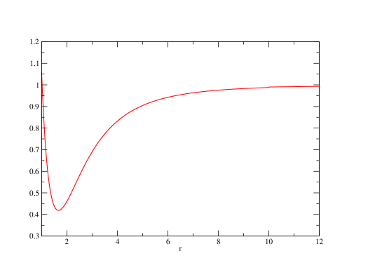
Figure 3: The potential $\frac{3W^{2}+H^{2}-1}{r^{2}}$ plotted against $r$, for $\lambda=0.1$.

The system (5.3) has the same generic form as the systems (3.21) and (3.20) studied in the previous section. We follow the same strategy in analysing it as we did in Sect. 4.3. Thus we first consider the bound state problem, where the right hand side of (5.3a) is set to zero, so that it is artificially decoupled from the system. The eigenvalue problem we need to solve is

$$\left(-\frac{d^{2}}{dr^{2}}+\frac{3W^{2}+H^{2}-1}{r^{2}}\right)w=\omega^{2}w.$$ (5.5)

As we saw in (5.4), the potential appearing here tends to the limiting value $1$ faster than in the Coulomb case but still according to an inverse square law, which is the threshold case for supporting infinitely many bound states, as discussed in in [21]. As shown there, the radial Schrödinger problem

$$-\frac{d^{2}w}{{dr}^{2}}+V(r)w=Ew,$$ (5.6)

where $V(r)\sim\frac{\beta}{r^{2}}$ for large $r$, has infinitely many bound states with $E<0$ if $\beta<-\frac{1}{4}$ (for $0>\beta\geq-\frac{1}{4}$ only a finite number of bound states are supported). Thus we expect infinitely many bound states with $\omega^{2}<1$ in (5.5), with all but the lowest values of $\omega^{2}$ lying very close to $1$. This poses problems for the NAG routine D02KEF, which requires a good initial estimate of the eigenvalue. Fortunately, the inverse square potential is a well-studied problem, and the WKB method provides an approximation for the ratio of successive eigenvalues [22]. Writing $\omega_{n}^{2}$ for the $n$-th eigenvalue in (5.5) we have the following formula, valid for large $n$:

$$\frac{\omega_{n}^{2}-1}{\omega_{n+1}^{2}-1}=e^{\frac{4\pi}{\sqrt{3}}}.$$ (5.7)

The first eigenvalue and eigenfunction is easily computed using the NAG routine D02KEF; the eigenfunction is displayed in Fig. 4. Initial guesses for subsequent eigenvalues can then be computed using (5.7). This approximation expected to be good only for large $n$, but worth using as an initial estimate in D02KEF for $n=2,3,4$. The computed eigenvalues, predicted values, and estimated error in computed value are displayed in Table 4. Rather surprisingly, the WKB guess even for $n=3$ is already accurate to 10 decimal places. The associated eigenfunctions are plotted in Fig. 5. They only show the exponential decay characteristic of bound state wavefunctions for rather large values of $r$, and we therefore plot them twice, using different scales.

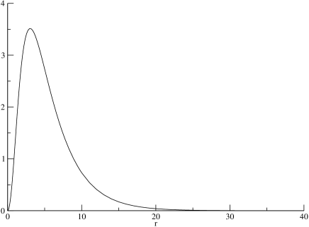
Figure 4: The lowest bound state of (5.5) for $\lambda=0.1$

$n$	1	2	3	4
$\omega_{n}$	0.95343	0.99998	0.999999985	0.999999999990
WKB prediction	n/a	0.99997	0.999999985	0.999999999989
$d\omega_{n}$	$0.38\times 10^{-6}$	$0.68\times 10^{-6}$	$0.63\times 10^{-10}$	$0.42\times 10^{-13}$

Table 4: Eigenvalues $\omega_{n}$ of (5.5) with $\lambda=0.1$, the predicted values for $n>1$ from 5.7, and the estimated accuracy $d\omega_{n}$ of the computed value $\omega_{n}$.

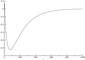
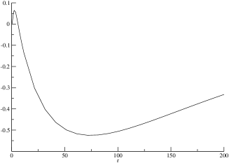
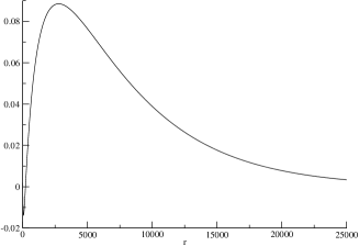
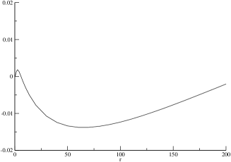
Figure 5: The 2nd (top) and third (bottom) bound state of (5.5), for $\lambda=0.1$. The scale on the right is chosen to show the first oscillation near the origin

As discussed in appendix A, the presence of bound states in (5.5) suggests the presence of (Feshbach) resonances in the radiative channel of the two channel problem (5.3). We now look for such resonances by studying the scattering associated with (5.3), in the energy range $\omega^{2}<1$. We follow the procedure summarised and used in Sect. 4.3. Thus we integrate (5.3) for $\lambda=0.1$ and a range of $\omega^{2}<1$, using the D02L suite of NAG routines for the integration. These solve initial value problems for ODEs using the Runge-Kutta-Nystrom method. We then tune the initial conditions with a shooting method to ensure that the function $w(r)$ decays at large $r$. The system has a regular singular point at the origin, which means that the numerical integration must start a little away from $r=0$. We make a series expansion of (5.3) about $r=0$ to find the correct initial data. We find that $w(r)\approx Ar^{2}$ and $h(r)\approx Br^{2}$ for real constants $A,B$, as in the $\lambda=0$ case.

We determine the ratio $A/B$ which allows $w$ to decay at infinity and integrate to compare the solution for $h$ at large distances to the spherical Bessel function $j_{0}$, as in (4.15) and to extract the phase shift $\delta(\omega)$. Our results are shown in Fig. 6. We see that as $\omega\to 1$, the phase shift $\delta$ increases sharply in value. An increase in $\delta$ by $\pi$ suggests a resonance. However, successive and closely spaced increases cannot easily be separated.

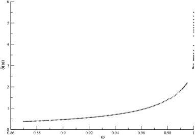
Figure 6: The phase shift $\delta(\omega)$ for the system (5.3)

In Fig. 7 we plot $\sin^{2}\delta$ as a function of $\omega$. We can clearly see one fairly wide resonance centred around $\omega=0.985$. Again, the accumulation of the bound state energies at 1, as shown in Table 4, makes it difficult to discern the interesting behaviour as $\omega\to 1$. We stretch out the region near threshold to see if there are, as we expect, more resonances as $\omega\to 1$. The result is plotted on the right in Fig. 7. We can see that there is at least one more resonant peak. We solved (5.3) for energies up to $\omega=0.999998$, which takes us past only the first two bound state energies in Table 4, thus the occurrence of two distinct resonance peaks in the scattering cross section is exactly what is expected. At higher energies the wavefunctions are extremely long range, of the order of $r=10^{6}$. Therefore, integrating for higher energies becomes increasingly time consuming. We expect, however, that each of infinitely many bound states of (5.5) will turn into resonances, and that infinitely many more resonant peaks in the scattering cross section arise as $\omega\to 1$.

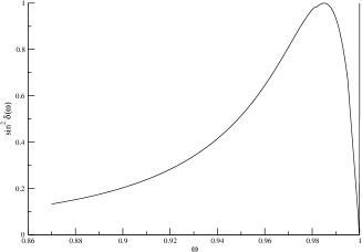
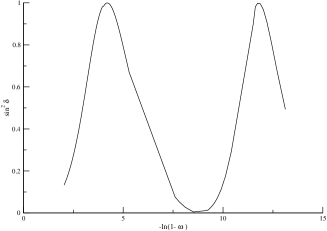
Figure 7: For the system (5.3), the function $\sin^{2}\delta$ is plotted as functions of $\omega$ (left) and as a function of $-\ln(1-\omega)$ (right).

6 Discussion and conclusion

The linearised YMH equations in the background of a ’t Hooft-Polyakov monopole have very interesting spectral properties. We have seen that there is a zero-energy bound state and an infinity of Coulomb bound states in the same energy region as an infinity of Feshbach resonances. For vanishing total angular momentum, there are two coupled systems which, despite their superficial similarity, have very different spectral properties: in one (called the Higgs system here) there are infinitely many Feshbach resonances, while in the other (called the photon system here) there are infinitely many true bound states, but no scattering states satisfying the background gauge condition and, in particular, no resonances. The occurrence of bound states can be understood in terms of a decoupling transformation. We also showed that the Feshbach resonances in the Higgs system persist when the Higgs self-coupling $\lambda$ is switched on. We saw that they become even more densely spaced, essentially because an attractive $1/r$ potential in the BPS limit is replaced by an attractive $1/r^{2}$ potential when $\lambda\neq 0$.

In this paper we restricted attention to the frequency range $\omega^{2}<1$ and to spherically symmetric perturbations (in the generalised sense). In this setting, the scattering is effectively single channel scattering, fully described by a single phase shift. When one goes beyond the threshold $\omega^{2}=1$, the scattering will be genuine two-channel scattering, whose study is more involved, both numerically and in terms of the interpretation of the results. However, very similar multi-channel scattering problems are much studied in atomic and nuclear physics, and were considered in [23] in the context of monopole scattering, so there is no problem in principle of carrying out a similar study here.

It would also be interesting to explore systems arising for larger eigenvalues of the generalised total angular momentum operator $\mathbf{J}$. The combination of our quaternionic formalism with the techniques developed in [5, 8, 24] should provide an efficient method for finding the corresponding systems of coupled differential equations. As explained in Sect. 3.2, we expect the system for $j=1$ to consist of ten equations, and for $j>2$ of twelve. However, a parity argument will split each of these system into two sub-systems (as it did in our $j=0$ case), so that the largest system one needs to consider has six channels.

To end, we point out the striking similarity between the spectral properties of the linearised YMH system in the background of the ’t Hooft-Polyakov monopole and those of the Laplace operator on the moduli space of charge two $SU(2)$ monopoles [23, 20]. The latter also include zero-energy bound states, Coulomb bound states embedded in the continuum and Feshbach resonance scattering. These similarities are likely to have an interpretation in terms of electric-magnetic duality. Spelling this out is left as the topic for a future investigation.

Appendix A Feshbach resonances

A Feshbach resonance [25] is a resonance in a system consisting of several channels in which a bound state occurs if the coupling(s) between the channels vanishes. Feshbach resonances are much studied in the context atomic physics [26] but also occur in other contexts, see [27] for a pedagogical and recent account.

Consider a simple system consisting of two channels with coupling terms including, for convenience, a parameter $0\leq q\leq 1$,

$$-\frac{1}{r}\frac{d^{2}}{dr^{2}}(ru)+V(r)u+qC(r)v =Eu,$$

$$-\frac{1}{r}\frac{d^{2}}{dr^{2}}(rv)+\hat{V}(r)v+qC(r)u =Ev.$$ (A.1)

We can decouple the equations by setting the parameter $q$ to zero. With $V<0$, suppose that the eigenvalue problem

$$-\frac{1}{r}\frac{d^{2}}{dr^{2}}(ru)+V(r)u=Eu$$ (A.2)

has bound states for $E<0$, occurring at $E_{0},E_{1},E_{2},\ldots$ but that those values are part of the continuous spectrum for the other decoupled equation

$$-\frac{1}{r}\frac{d^{2}}{dr^{2}}(rv)+\hat{V}(r)v=Ev.$$ (A.3)

When the coupling parameter $q$ is non-zero, the bound states in (A.2) can leak into the radiative channel (A.3) and decay. When that happens, Feshbach resonances in (A) generically occur at values close to $E_{0},E_{1},E_{2},\ldots$. Examples of such resonances are studied in [15] and [23], both in the context of magnetic monopoles. A single channel eigenvalue problem such as (A.2) is generally much easier to solve than a two channel coupled problem such as (A). Hence, it is worth looking at the bound state problem, as it gives an idea of where the resonances will occur. In systems where the coupling terms are weaker at large distances than the potential, the decoupled problem is a good approximation. Then these preliminary calculations mean that the region of searching for resonances is narrowed down, so that computational time is reduced.

References

- [1] R. Rajaraman. Solitons and Instantons. Elsevier Science, Amsterdam, 1987.
- [2] T. H. R. Skyrme, A non-linear field theory. Proc. R. Soc. Lond. A260:127, 1961
- [3] T. H. R. Skyrme, A unified field theory of mesons and baryons. Nucl. Phys. 31:556, 1962
- [4] N. Manton and P. Sutcliffe, Topological Solitons. Cambridge Monographs on Mathematical Physics, Cambridge University Press, Cambridge, 2004.
- [5] R. Jackiw and C. Rebbi. Solitons with fermion number 1/2. Phys. Rev., D13:3398–3409, 1976.
- [6] E. J. Weinberg, Parameter Counting for Multi-Monopole Solutions, Phys. Rev., D20:936–944, 1979.
- [7] C. Callias, Axial anomalies and index theorems on open spaces, Comm. Math. Phys., 62:213, 1978.
- [8] F. A. Bais and W. Troost. Zero modes and bound states of the supersymmetric monopole. Nucl. Phys., B178:125, 1981.
- [9] V. A. Rubakov, Superheavy Magnetic Monopoles and Proton Decay. JETP Lett. 33:644-646, 1981,
- [10] V. A. Rubakov, Adler-Bell-Jackiw Anomaly and Fermion Number Breaking in the Presence of a Magnetic Monopole. Nucl.Phys. B203:311-348, 1982..
- [11] C. G. Callan, Dyon-Fermion Dynamics, Phys.Rev. D26:2058-2068, 1982.
- [12] W. J. Marciano and I. J. Muzinich, Exact Solution of the Dirac Equation in the Field of a ’t Hooft-Polyakov Monopole Phys. Rev. Lett. 50:1035–1037, 1983.
- [13] G. Fodor and I. Rácz. What does a strongly excited ’t Hooft-Polyakov magnetic monopole do? Phys. Rev. Lett., 92:151801, 2004.
- [14] G. Fodor and I. Rácz. Numerical investigation of highly excited magnetic monopoles in SU(2) Yang-Mills-Higgs theory. Phys. Rev. D, 77:025019, 2008.
- [15] P. Forgács and M. S. Volkov. Resonant excitations of the ’t Hooft-Polyakov monopole. Phys. Rev. Lett., 92:151802, 2004.
- [16] G. ’t Hooft. Magnetic monopoles in unified gauge theories. Nucl. Phys., B79:276–284, 1974.
- [17] A. M. Polyakov. Particle spectrum in quantum field theory. JETP Lett., 20:194–195, 1974.
- [18] M. K. Prasad and C. M. Sommerfield. An exact classical solution for the ’t Hooft monopole and the Julia-Zee dyon. Phys. Rev. Lett., 35:760–762, 1975.
- [19] E. B. Bogomol’nyi. Stability of classical solutions. Sov. J. Nucl. Phys., 24:449, 1976.
- [20] N. S. Manton and B. J. Schroers. Bundles over moduli spaces and the quantization of BPS monopoles. Ann. Phys., 225:290–338, 1993.
- [21] L. D. Landau and E. M. Lifshitz. Quantum mechanics: non-relativistic theory. Course of Theoretical Physics, Vol. 3. Addison-Wesley Series in Advanced Physics. Pergamon Press Ltd., London-Paris, 1958.
- [22] M. J. Moritz, C. Eltschka, and H. Friedrich. Threshold properties of attractive and repulsive potentials. Phys. Rev. A, 63(4):042102, 2001.
- [23] B. J. Schroers. Quantum scattering of BPS monopoles at low-energy. Nucl. Phys., B367:177–216, 1991.
- [24] S. Majid, Partial waves for the linearised Yang-Mills equation about a monopole background, J. Math. Phys. 30:1150–1157, 1989.
- [25] H. Feshbach. Ann. Phys. (N.Y.), 5: 357, 1958.
- [26] M. H. Mittleman. Resonances in multichannel scattering. Phys. Rev., 147:73–76, 1966.
- [27] J. N. Milstein, From Cooper pairs to molecules: Effective field theories for ultra-cold atomic gases near Feshbach resonances, PhD Thesis, JILA, University of Colorado, Boulder, 2004 .