INSTITUT NATIONAL DE RECHERCHE EN INFORMATIQUE ET EN AUTOMATIQUE

List-decoding of binary Goppa codes up to the binary Johnson bound
Daniel Augot — Morgan Barbier — Alain CouvreurN° 7490
 Décembre 2010 

Abstract: We study the list-decoding problem of alternant codes, with the notable case of classical Goppa codes. The major consideration here is to take into account the size of the alphabet, which shows great influence on the list-decoding radius. This amounts to compare the generic Johnson bound to the $q$-ary Johnson bound. This difference is important when $q$ is very small.

Essentially, the most favourable case is $q=2$, for which the decoding radius is greatly improved, notably when the relative minimum distance gets close to $1/2$.

Even though the announced result, which is the list-decoding radius of binary Goppa codes, is new, it can be rather easily made up from previous sources (V.  Guruswami, R. M. Roth and I. Tal, R .M. Roth), which may be a little bit unknown, and in which the case of binary Goppa codes has apparently not been thought at. Only D. J. Bernstein treats the case of binary Goppa codes in a preprint. References are given in the introduction.

We propose an autonomous treatment and also a complexity analysis of the studied algorithm, which is quadratic in the blocklength $n$, when decoding at some distance of the relative maximum decoding radius, and in $\mathcal{O}(n^{7})$ when reaching the maximum radius.

Key-words: Error correcting codes, algebraic geometric codes, list-decoding, alternant codes, binary Goppa codes

Décodage en liste des codes de Goppa binaires jusqu’à la borne de Johnson binaire

Résumé : Nous étudions le décodage en liste des codes alternants, dont notamment les codes de Goppa classiques. La considération majeure est de prendre en compte la taille de l’alphabet, qui influe sur la capacité de correction, surtout dans le cas de l’alphabet binaire. Cela revient à comparer la borne de Johnson que nous appelons générique, à la borne de Johnson que nous appelons $q$-aire, qui prend en compte la taille $q$ du corps. Cette différence est d’autant plus sensible que $q$ est petit.

Essentiellement, le cas le plus favorable est celui de l’alphabet binaire pour lequel on peut augmenter significativement le rayon du décodage en liste. Et ce, d’autant plus que la distance minimale relative construite du code alternant binaire est proche de $1/2$.

Bien que le résultat annoncé ici, à savoir le rayon de décodage en liste des codes de Goppa binaires, soit nouveau, il peut assez facilement être déduit de sources relativement peu connues (V.  Guruswami, R. M. Roth and I. Tal, R .M. Roth) et dont les auteurs n’ont apparemment pas pensé à aborder les codes de Goppa binaires. Seul D. J. Bernstein a traité le décodage en liste des codes de Goppa dans une prépublication. Les références sont données dans l’introduction.

Nous proposons un contenu autonome, et aussi une analyse de la complexité de l’algorithme étudié, qui est quadratique en la longueur $n$ du code, si on se tient à distance du rayon relatif de décodage maximal, et en $\mathcal{O}(n^{7})$ pour le rayon de décodage maximal.

Mots-clés : Codes correcteurs d’erreur, codes géométriques, décodage en liste, codes alternants, codes de Goppa binaires

1 Introduction

In 1997, Sudan presented the first list-decoding algorithm for Reed-Solomon codes [Sud97] having a low, yet positive, rate. Since the correction radius of Sudan’s algorithm for these codes is larger than the one obtained by unambiguous decoding algorithms, this represented an important milestone in list-decoding, which was previously studied at a theoretical level. See [Eli91] and references therein for considerations on the “capacity” of list-decoding. Afterwards, Guruswami and Sudan improved the previous algorithm by adding a multiplicity constraint in the interpolation procedure. These additional constraints enable to increase the correction radius of Sudan’s algorithm for Reed-Solomon codes of any rate [GS99]. The number of errors that this algorithm is able to list-decode corresponds to the Johnson radius $e_{\infty}(n,d)=\left\lceil n-\sqrt{n(n-d)}\right\rceil-1$, where $d$ is the minimum distance of the code.

Actually, when the size $q$ of the alphabet is properly taken into account $q$, the bound is improved up to

$$e_{q}(n,d)=\left\lceil\theta_{q}\left(n-\sqrt{n\left(n-\frac{d}{\theta_{q}}\right)}\right)\right\rceil-1,$$

where $\theta_{q}=1-\frac{1}{q}$. See [Gur07, Chapter 3] for a complete discussion about these kinds of bounds, relating the list-decoding radius to the minimum distance. Dividing by $n$, and taking relative values, with $\delta=\frac{d}{n}$, we define $\tau_{\infty}(\delta)=\frac{e_{\infty}(n,d)}{n}$, and $\tau_{q}(\delta)=\frac{e_{q}(n,d)}{n}$, which are

$$\tau_{\infty}(\delta)=1-\sqrt{1-\delta},\quad\tau_{q}(\delta)=\theta_{q}\left(1-\sqrt{1-\frac{\delta}{\theta_{q}}}\right)$$ (1)

Note that $\tau_{q}(\delta)$ gets decreasingly close to $\tau_{\infty}(\delta)$ when $q$ grows, and that $\tau_{2}(n,q)$ is the largest, see Figure 1. We call $\tau_{\infty}(\delta)$ the generic Johnson bound, which does not take into account the size of the field, and indeed works over any field, finite or not. We refer to $\tau_{q}(\delta)$ as the $q$-ary Johnson bound, where the influence of $q$ is properly reflected.

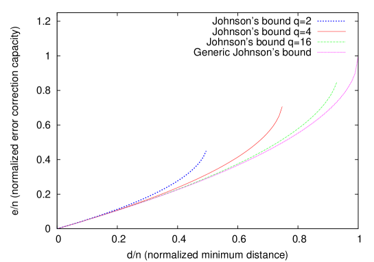
Figure 1: Comparison of the limit generic Johnson bound $\tau_{\infty}(\delta)$ and the limit $q$-ary Johnson bounds $\tau_{q}(\delta)$, for small $q$. Note that the each curve ends at $\delta=\theta_{q}=1-\frac{1}{q}$, which is the maximum relative minimum distance of codes of positive rates over $\mathbb{F}_{q}$, from the Plotkin bound.

The truth is that the $\tau_{q}(\delta)$ radius can be reached for the whole class of alternant codes, and this paper presents how to do this. We have essentially compiled existing, but not very well-known results, with the spirit of giving a report on the issue of list-decoding classical algebraic codes over bounded alphabets. First, we have to properly give credits.

Considering the possibility of varying multiplicities, Koetter and Vardy proposed in 2001, an algebraic soft-decision decoding algorithm for Reed-Solomon codes [KV03]. This method is based on an interpolation procedure which is similar to Guruswami-Sudan’s algorithm, except that the set of interpolation points is two dimensional, and may present varying multiplicities, according the reliability measurements given by the channel. Note that the idea of varying multiplicities was also considered in [GS99], as the “weighted polynomial reconstruction problem”, but was not instantiated for particular cases, as it was done by Koetter and Vardy. Before the publication of [KV03], also circulated a preprint of Koetter and Vardy [VK00], which was a greatly extended version of [KV03], with many possible interesting instances of the weighted interpolation considered. In particular, the authors discussed the decoding of BCH codes over the binary symmetric channel, and reached in fact an error capacity which is nothing else than $\tau_{2}(\delta)$. Note that BCH codes are nothing else than alternant codes, with benefits when the alphabet is $\mathbb{F}_{2}$. This was not published.

Guruswami-Sudan’s algorithm is in fact very general and can also be applied to (one point) Algebraic Geometric codes as also shown by Guruswami and Sudan in [GS99]. By this manner, one also reaches the Johnson radius $\left\lceil n-\sqrt{n(n-d^{\star})}\right\rceil-1$, where $d^{\star}$ is the Goppa designed distance. Contrarily to Reed-Solomon codes, it is possible, for a fixed alphabet $\mathbb{F}_{q}$, to construct Algebraic Geometric codes of any length. In this context, it makes sense to try to reach the $q$-ary Johnson bound $\tau_{q}(\delta)$, which is done in Guruswami’s thesis [Gur04], at the end of Chapter 6.

Apparently independently, Roth and Tal considered the list-decoding problem in [TR03], but only an one page abstract. Roth’s book [Rot06], where many algebraic codes are presented through the prism of alternant codes, considers the list-decoding of these codes and shows how to reach the $q$-ary Johnson radius $\tau_{q}(\delta)$, where $\delta$ is the minimum distance of the Generalised Reed-Solomon code from which the alternant code is built. Note that alternant codes were considered in [GS99], but only the generic Johnson Bound $\tau_{\infty}(\delta)$ was discussed there.

Among the alternant codes, the binary Goppa codes are particularly important. They are not to be confused with Goppa’s Algebraic Geometric codes, although there is a strong connection which is developed in Section 4. These codes are constructed with a Goppa polynomial $G(X)$ of degree $r$ and if this polynomial is square-free, then the distance of these codes is at least $2r+1$ which is almost the double of $r$, which is what would be expected for a generic alternant code. In fact, using the statements in [Rot06], and using the fact that the Goppa code built with $G(X)$ is the same as the Goppa code built with $G(X)^{2}$, it is explicit that these codes can be list-decoded up to the radius

$$\left\lceil\frac{1}{2}\left(n-\sqrt{n\left(n-(4r+2)\right)}\right)\right\rceil-1.$$ (2)

But actually, the first author who really considered the list-decoding of binary Goppa codes is D. J. Bernstein [Ber08], in a preprint which can be found on his personal web page. He uses a completely different approach than interpolation based list-decoding algorithms, starting with Patterson’s algorithm [Pat75] for decoding classical Goppa codes. Patterson’s algorithm is designed to decode up to $t$ errors, and to list-decode further, Bernstein reuses the information obtained by an unsuccessful application of Patterson’s algorithm in a smart way. It is also the approach used by Wu [Wu08] in his algorithm for list-decoding Reed-Solomon and BCH codes, where the Berlekamp-Massey algorithm is considered instead of Patterson’s algorithm. Notice that Wu can reach the binary Johnson bound $\tau_{2}(\delta)$, using very particular properties of Berlekamp-Massey algorithm for decoding binary BCH codes [Ber68, Ber84]. However, Wu’s approach can apparently not be straightforwardly applied to Goppa codes.

Organisation of the paper

Section 2 is devoted to recall the list-decoding problem, the Johnson bounds generic or $q$-ary, and Section 3 to the definitions of the codes we wish to decode, namely alternant codes and classical Goppa codes. Section 4 shows how to consider classical Goppa codes as subfield subcodes of Algebraic Geometric Goppa codes. Then, using Guruswami’s result in [Gur04], it is almost straightforward to show that these codes can be decoded up to the binary Johnson bound $e_{2}(n,d^{\star})$, where $d^{\star}=2r+1$. However, this approach is far reaching, and the reader may skip Section 4, since Section 5 provides a self-contained treatment of the decoding of alternant codes up to the $q$-ary Johnson bound. Essentially, this amounts to show how to pick the varying multiplicities, but we also study the dependency on the multiplicity. This enables us to give an estimation of the complexity of the decoding algorithm, which is quadratic in the length $n$ of the code, when one is not too greedy.

2 List-decoding

First, recall the notion of list-decoding and multiplicity.

Problem 2.1.

Let $\mathcal{C}$ be a code in its ambient space $\mathbb{F}_{q}^{n}$. The list-decoding problem of $\mathcal{C}$ up to the radius $e\in[0,n]$ consists, for any $y$ in $\mathbb{F}_{q}^{n}$, in finding all the codewords $c$ in $\mathcal{C}$ such that $d(c,y)\leq e$.

The main question is: how large can $e$ be, such that the list keeps a reasonable size? A partial answer is given by the so-called Johnson bound.

3 Classical Goppa Codes

This section is devoted to the study of classical $q$–ary Goppa codes, regarded as alternant codes (subfield subcodes of Generalised Reed–Solomon codes) and as subfield subcodes of Algebraic Geometric codes. Afterwards, using Guruswami’s results [Gur04] on soft-decoding of Algebraic Geometric codes, we prove that classical Goppa codes can be list-decoded in polynomial time up to the $q$–ary Johnson bound.

Context

In this section, $q$ denotes an arbitrary prime power and $m,n$ denote two positive integers such that $m\geq 2$ and $n\leq q^{m}$. In addition $L\triangleq(\alpha_{1},\ldots,\alpha_{n})$ denotes an $n$–tuple of distinct elements of $\mathbb{F}_{q^{m}}$.

3.1 Classical Goppa codes

Definition 3.1.

Let $r$ be an integer such that $0<r<n$. Let $G\in\mathbb{F}_{q^{m}}[X]$ be a polynomial of degree $r$ which does not vanish at any element of $L$. The $q$–ary classical Goppa code $\Gamma_{q}(L,G)$ is defined by

$$\Gamma_{q}(L,G)\triangleq\left\{(c_{1},\ldots,c_{n})\in\mathbb{F}_{q}^{n}\ \left|\ \sum_{i=1}^{n}\frac{c_{i}}{X-\alpha_{i}}\equiv 0\ \textrm{mod}\ (G(X))\right.\right\}\cdot$$

3.2 Classical Goppa codes are alternant

Definition 3.2 (Evaluation map).

Let $B\triangleq(\beta_{1},\ldots,\beta_{n})$ be an $n$–tuple of elements of $\mathbb{F}_{q^{m}}^{\times}$, and $L\triangleq(\alpha_{1},\ldots,\alpha_{n})$ denotes an $n$–tuple of distinct elements of $\mathbb{F}_{q^{m}}$. The associated evaluation map is:

$$\operatorname{ev}:\left\{\begin{array}[]{ccc}\mathbb{F}_{q^{m}}[X]&\rightarrow&\mathbb{F}_{q^{m}}^{n}\\ f(X)&\mapsto&(\beta_{1}f(\alpha_{1}),\ldots,\beta_{n}f(\alpha_{n}))\end{array}\right..$$

Definition 3.3 (Generalised Reed–Solomon code).

Let $B\triangleq(\beta_{1},\ldots,\beta_{n})$ be an $n$–tuple of elements of $\mathbb{F}_{q^{m}}^{\times}$. Let $k$ be a positive integer. The Generalised Reed–Solomon code (or GRS code) over $\mathbb{F}_{q^{m}}$ associated to the triple $(L,B,k)$ is the code:

$$GRS_{q^{m}}(L,B,k)\triangleq\left\{\operatorname{ev}(f(X))\ |\ f\in\mathbb{F}_{q^{m}}[X]_{<k}\right\},$$

where $\operatorname{ev}$ denotes the evaluation map in Definition 3.2. This code has parameters $[n,k,n-k+1]_{q^{m}}$ ([MS83] $Ch10,\S 8,p303$ ).

Definition 3.4 (Subfield Subcode).

Let $K$ be a finite field and $M/K$ be a finite extension of it. Let $\mathcal{C}$ be a code of length $n$ with coordinates in $M$, the subfield subcode $\mathcal{C}_{|K}$ of $\mathcal{C}$ is the code

$$\mathcal{C}_{|K}\triangleq\mathcal{C}\cap K^{n}.$$

Definition 3.5 (Alternant code).

A code is said to be alternant if it is a subfield subcode of a GRS code.

In particular, classical $q$–ary Goppa codes are alternant. Let us describe a GRS code over $\mathbb{F}_{q^{m}}$ whose subfield subcode over $\mathbb{F}_{q}$ is $\Gamma_{q}(L,G)$.

Proposition 3.6.

Let $r$ be an integer such that $0<r<n$ and $G\in\mathbb{F}_{q^{m}}[X]$ be a polynomial of degree $r$ which does not vanish at any element of $L$. Then, the classical Goppa code $\Gamma_{q}(L,G)$ is the subfield subcode $GRS_{q^{m}}(L,B,n-r)_{|\mathbb{F}_{q}}$, where $B=(\beta_{1},\ldots,\beta_{n})$ is defined by

$$\forall i\in\{1,\ldots,n\},\ \beta_{i}\triangleq\frac{G(\alpha_{i})}{\prod_{j\neq i}(\alpha_{i}-\alpha_{j})}\cdot$$

Proof.

See [MS83] $Ch12,\S 3,p340,Thm4$.

∎

3.3 A property on the minimum distance of classical Goppa codes

Let $L\triangleq(\alpha_{1},\ldots,\alpha_{n})$ be an $n$–tuple of distinct elements of $\mathbb{F}_{q^{m}}$ and $G\in\mathbb{F}_{q^{m}}[X]$ be a polynomial of degree $r>0$ which does not vanish at any element of $L$. Since $\Gamma_{q}(L,G)$ is the subfield subcode of a GRS code with parameters $[n,n-r,r+1]_{q^{m}}$, the code $\Gamma_{q}(L,G)$ has parameters $[n,\geq n-mr,\geq r+1]_{q}$ (see [Sti93] Lemma VIII.1.3 and [MS83] $Ch12,\S 3,p339$).

In addition, it is possible to get a better estimate of the minimum distance in some situations. This is the objective of the following result.

Theorem 3.7.

Let $L\triangleq(\alpha_{1},\ldots,\alpha_{n})$ be an $n$–tuple of distinct elements of $\mathbb{F}_{q^{m}}$. Let $G\in\mathbb{F}_{q^{m}}[X]$ be square-free polynomial which does not vanish at any element of $L$ and such that $0<\deg(G)<n/q$. Then,

$$\Gamma_{q}(L,G^{q-1})=\Gamma_{q}(L,G^{q}).$$

Proof.

[BLP10] Theorem 4.1. ∎

The codes $\Gamma_{q}(L,G^{q-1})$ and $\Gamma_{q}(L,G^{q})$ are subfield subcodes of two distinct GRS codes but are equal. The GRS code associated to $G^{q-1}$ has a larger dimension than the one associated to $G^{q}$ but a smaller minimum distance. Thus, it is interesting to deduce a lower bound for the minimum distance from the GRS code associated to $G^{q}$ and a lower bound for the dimension from the one associated to $G^{q-1}$.

This motivates the following definition.

Definition 3.8.

In the context of Theorem 3.7, the designed minimum distance of $\Gamma_{q}(L,G^{q-1})$ is $d_{\textrm{Gop}}^{\star}\triangleq q\deg(G)+1$. It is a lower bound for the actual minimum distance.

Remark 3.9.

Using almost the same proof, Theorem 3.7 can be generalised as: let $G_{1},\ldots,G_{t}$ be irreducible polynomials in $\mathbb{F}_{q^{m}}[X]$ and $e_{1},\ldots,e_{t}$ are positive integers congruent to $-1\mod q$, then $\Gamma_{q}(L,G_{1}^{e_{1}}\cdots G_{t}^{e_{t}})=\Gamma_{q}(L,G_{1}^{e_{1}+1}\cdots G_{t}^{e_{t}+1})$.

4 List-decoding of classical Goppa Codes as Algebraic Geometric codes

In this section, $C$ denotes a smooth projective absolutely irreducible curve over a finite field $\mathbb{F}_{q}$. Its genus is denoted by $g(C)$.

4.1 Prerequisites in algebraic geometry

The main notions of algebraic geometry used in this article are summarised in what follows. For further details, we refer the reader to [Ful89] for theoretical results on algebraic curves and to [Sti93] and [VNT07] for classical notions on Algebraic Geometric codes.

Points and divisors

If $k$ is an algebraic extension of the base field $\mathbb{F}_{q}^{m}$, we denote by $C(k)$ the set of $k$–rational points of $C$, that is the set of points whose coordinates are in $k$.

The group of divisors $\textrm{Div}_{\overline{\mathbb{F}}_{q}}(C)$ of $C$ is the free abelian group generated by the geometric points of $C$ (i.e. by $C(\overline{\mathbb{F}}_{q})$). Elements of $\textrm{Div}_{\overline{\mathbb{F}}_{q}}(C)$ are of the form $\mathcal{G}=\sum_{P\in C(\overline{\mathbb{F}}_{q})}a_{P}P$, where the $a_{P}$’s are integers and are all zero but a finite number of them. The support of $\mathcal{G}=\sum a_{P}P$ is the finite set

$$\textrm{Supp}(\mathcal{G})\triangleq\{P\in C(\overline{\mathbb{F}}_{q})\ |\ a_{P}\neq 0\}.$$

The group $\textrm{Div}_{\mathbb{F}_{q}}(C)$ of $\mathbb{F}_{q}$–rational divisors is the subgroup of $\textrm{Div}_{\overline{\mathbb{F}}_{q}}(C)$ of divisors which are fixed by the Frobenius map.

A partial order is defined on divisors:

$$\mathcal{D}=\sum d_{P}P\geq\mathcal{E}=\sum e_{P}P\ \Leftrightarrow\ \forall P\in C(\overline{\mathbb{F}}_{q}),\ d_{P}\geq e_{P}.$$

A divisor $\mathcal{D}=\sum d_{P}P$ is said to be effective or positive if $\mathcal{D}\geq 0$, i.e. if for all $P\in C(\overline{\mathbb{F}}_{q})$, $d_{P}\geq 0$. To each divisor $\mathcal{D}=\sum_{P}d_{P}P$, we associate its degree $\deg(\mathcal{D})\in{\mathbb{Z}}$ defined by $\deg(\mathcal{D})\triangleq\sum d_{P}$. This sum makes sense since the $d_{P}$’s are all zero but a finite number of them.

Rational functions

The field of $\mathbb{F}_{q}$–rational functions on $C$ is denoted by $\mathbb{F}_{q}(C)$. For a nonzero function $f\in\mathbb{F}_{q}(C)$, we associate its divisor

$$(f)\triangleq\sum_{P\in C(\overline{\mathbb{F}}_{q})}v_{P}(f).P,$$

where $v_{P}$ denotes the valuation at $P$. This sum is actually finite since the number of zeroes and poles of a function is finite. Such a divisor is called a principal divisor. The positive part of $(f)$ is called the divisor of the zeroes of $f$ and denoted by

$${(f)}_{0}\triangleq\sum_{P\in C(\overline{\mathbb{F}}_{q}),\ v_{P}(f)>0}v_{P}(f).P.$$

Lemma 4.1.

The degree of a principal divisor is zero.

Proof.

[Ful89] Chapter 8 Proposition 1. ∎

Riemann–Roch spaces

Given a divisor $\mathcal{G}\in\textrm{Div}_{\mathbb{F}_{q}}(C)$, one associates a vector space of rational functions defined by $L(\mathcal{G})\triangleq\{f\in\mathbb{F}_{q}(C)\ |\ (f)\geq-\mathcal{G}\}\cup\{0\}.$ This space is finite dimensional and its dimension is bounded below from the Riemann–Roch theorem $\dim(L(\mathcal{G}))\geq\deg(\mathcal{G})+1-g(C).$ This inequality becomes an equality if $\deg(\mathcal{G})>2g(C)-2$.

4.2 Construction and parameters of Algebraic Geometric codes

Definition 4.2.

Let $\mathcal{G}$ be an $\mathbb{F}_{q}$–rational divisor on $C$ and $P_{1},\ldots,P_{n}$ be a set of distinct rational points of $C$ avoiding the support of $\mathcal{G}$. Denote by $\mathcal{D}$ the divisor $\mathcal{D}\triangleq P_{1}+\cdots+P_{n}$. The code $\mathcal{C}_{L}(\mathcal{D},\mathcal{G})$ is the image of the map

$$\textrm{ev}_{\mathcal{D}}:\left\{\begin{array}[]{ccc}L(\mathcal{G})&\rightarrow&\mathbb{F}_{q}^{n}\\ f&\mapsto&(f(P_{1}),\ldots,f(P_{n}))\end{array}\right..$$

The parameters of Algebraic Geometric codes (or AG codes) can be estimated using the Riemann–Roch theorem and Lemma 4.1.

Proposition 4.3.

In the context of Definition 4.2, assume that $\deg(\mathcal{G})<n$. Then the code $\mathcal{C}_{L}(\mathcal{D},\mathcal{G})$ has parameters $[n,k,d]_{q}$ where $k\geq\deg(\mathcal{G})+1-g(C)$ and $d\geq n-\deg(\mathcal{G})$. Moreover, if $2g(C)-2<\deg(\mathcal{G})$, then $k=\deg(\mathcal{G})+1-g(C)$.

Proof.

[Sti93] Proposition II.2.2 and Corollary II.2.3. ∎

Definition 4.4 (Designed distance of an AG code).

The designed distance of $\mathcal{C}_{L}(\mathcal{D},\mathcal{G})$ is $d_{\textrm{AG}}^{\star}\triangleq n-\deg(\mathcal{G})$.

4.3 Classical Goppa codes as Algebraic Geometric codes

In general, one can prove that the GRS codes are the AG codes on the projective line (see [Sti93] Proposition II.3.5). Therefore, from Proposition 3.6, classical Goppa codes are subfield subcodes of AG codes. In what follows we give an explicit description of the divisors used to construct a classical Goppa code $\Gamma_{q}(L,G)$ as a subfield subcode of an AG code.

Context

The context is that of Section 3. In addition, $P_{1},\ldots,P_{n}$ are the points of ${\mathbb{P}}^{1}$ of respective coordinates $(\alpha_{1}:1),\ldots,(\alpha_{n}:1)$ and $P_{\infty}$ is the point “at infinity” of coordinates $(1:0)$. We denote by $\mathcal{D}$ the divisor $\mathcal{D}\triangleq P_{1}+\cdots+P_{n}\in\textrm{Div}_{\mathbb{F}_{q^{m}}}({\mathbb{P}}^{1})$. Finally, we set

$$F(X)\triangleq\prod_{i=1}^{n}(X-\alpha_{i})\ \in\mathbb{F}_{q^{m}}[X].$$ (3)

Remark 4.5.

A polynomial $H\in\mathbb{F}_{q}[X]$ of degree $d$ can be regarded as a rational function on ${\mathbb{P}}^{1}$ having a single pole at $P_{\infty}$ with multiplicity $d$. In particular $\deg(H)\leq d\Leftrightarrow(H)\geq-dP_{\infty}\Leftrightarrow H\in L(-dP_{\infty})$.

Theorem 4.6.

Let $G\in\mathbb{F}_{q^{m}}[X]$ be a polynomial of degree $r$ such that $0<r<n$. Then,

$$\Gamma_{q}(L,G)=\mathcal{C}_{L}(\mathcal{D},\mathcal{A}-\mathcal{E})_{|\mathbb{F}_{q}},$$

where $\mathcal{A},\mathcal{E}$ are positive divisors defined by $\mathcal{E}\triangleq{(G)}_{0}$ and $\mathcal{A}\triangleq{(F^{\prime})}+(n-1)P_{\infty}$, where $F^{\prime}$ denotes the derivative of $F$.

Remark 4.7.

The above result is actually proved in [Sti93] (Proposition II.3.11) but using another description of classical Goppa codes (based on their parity–check matrices). Therefore, we chose to give another proof corresponding better to the present description of classical Goppa codes.

Proof of Theorem 4.6.

First, let us prove that $\mathcal{A}$ is well-defined and positive. Since $F$ has simple roots (see (3)), it is not a $p$–th power in $\mathbb{F}_{q^{m}}[X]$ (where $p$ denotes the characteristic). Thus, $F^{\prime}$ is nonzero. Moreover $F^{\prime}$ has degree $\leq n-1$ (with equality if and only if $n-1$ is prime to the characteristic). Remark 4.5 entails $(F^{\prime})\geq-(n-1)P_{\infty}$ and $\mathcal{A}=(F^{\prime})+(n-1)P_{\infty}\geq 0$.

Let us prove the result. Thanks to Proposition 3.6, it is sufficient to prove that $\mathcal{C}_{L}(\mathcal{D},\mathcal{A}-\mathcal{E})=GRS_{q^{m}}(L,B,n-r)$, where $B=(\beta_{1},\ldots,\beta_{n})$ with

$$\forall i\in\{1,\ldots,n\},\ \beta_{i}\triangleq\frac{G(\alpha_{i})}{\prod_{j\neq i}(\alpha_{i}-\alpha_{j})}\cdot$$ (4)

Notice that,

$$\forall i\in\{1,\ldots,n\},\ F^{\prime}(\alpha_{i})=\prod_{j\neq i}(\alpha_{i}-\alpha_{j}).$$ (5)

Let $H$ be a polynomial in $\mathbb{F}_{q^{m}}[X]_{<n-r}$. Remark 4.5 yields $(H)\geq-(n-r-1)P_{\infty}$ and

$$\begin{array}[]{rcl}\left(\frac{\displaystyle GH}{\displaystyle F^{\prime}}\right)=(G)+(H)-(F^{\prime})&\geq&(\mathcal{E}-rP_{\infty})-(n-r-1)P_{\infty}-\mathcal{A}+(n-1)P_{\infty}\\ &\geq&-(\mathcal{A}-\mathcal{E}).\end{array}$$

Thus, $GH/F^{\prime}\in L(\mathcal{A}-\mathcal{E})$ and, from (4) and (5), we have

$$\frac{GH}{F^{\prime}}(\alpha_{i})=\beta_{i}H(\alpha_{i}).$$

This yields $GRS_{q^{m}}(L,B,n-r)\subseteq\mathcal{C}_{L}(\mathcal{D},\mathcal{A}-\mathcal{E})$.

For the reverse inclusion, we prove that both codes have the same dimension. The dimension of $GRS_{q^{m}}(L,B,n-r)$ is $n-r$. For $\mathcal{C}_{L}(\mathcal{D},\mathcal{A}-\mathcal{E})$, we first compute $\deg(\mathcal{A}-\mathcal{E})$. By definition, $\deg(\mathcal{A})=\deg((F^{\prime}))+n-1$ which equals $n-1$ from Lemma 4.1. The degree of $\mathcal{E}$ is that of the polynomial $G$, that is $r$. Thus, $\deg(\mathcal{A}-\mathcal{E})=n-1-r$. Since $r$ is assumed to satisfy $0<r<n$ and since the genus of ${\mathbb{P}}^{1}$ is zero, we have $2g(C)-2=-2<\deg(\mathcal{A}-\mathcal{E})<n.$ Finally, Proposition 4.3 entails $\dim\mathcal{C}_{L}(\mathcal{D},\mathcal{A}-\mathcal{E})=\deg(\mathcal{A}-\mathcal{E})+1-g(C)=n-r$, which concludes the proof. ∎

Remark 4.8.

Another and in some sense more natural way to describe $\Gamma_{q}(L,G)$ as a subfield subcode of an AG code is to use differential forms on ${\mathbb{P}}^{1}$. By this way, one proves easily that $\Gamma_{q}(L,G)=\mathcal{C}_{\Omega}(\mathcal{D},\mathcal{E}-P)_{|\mathbb{F}_{q}}$. Then, considering the differential form $\nu\triangleq\frac{dF}{F}$, one can prove that its divisor is $(\nu)=\mathcal{A}-\mathcal{D}-P_{\infty}$. Afterwards, using [Sti93] Proposition II.2.10, we get

$$\mathcal{C}_{\Omega}(\mathcal{D},\mathcal{E}-P)=\mathcal{C}_{L}(\mathcal{D},(\nu)-\mathcal{E}+P+\mathcal{D})=\mathcal{C}_{L}(\mathcal{D},\mathcal{A}-\mathcal{E}).$$

The main tool for the proof of the list-decodability of classical Goppa codes is a Theorem on the soft-decoding of AG codes, this is the reason why we introduce our list-decoding algorithm by an Algebraic Geometric codes point of view.

4.4 List-decoding up to the $q$-ary Johnson radius

Theorem 4.9 ([Gur04] Theorem 6.41).

For every $q$-ary AG-code $\mathcal{C}$ of block-length $n$ and designed minimum distance $d^{\star}=n-\alpha$, there exists a representation of the code of size polynomial in $n$ under which the following holds. Let $\varepsilon>0$ be an arbitrary constant. For $1\leq i\leq n$ and $\lambda\in\mathbb{F}_{q}$ , let $w_{i,\lambda}$ be a non-negative real. Then one can find in $poly(n,q,1/\varepsilon)$ time, a list of all codewords $c=(c_{1},c_{2},\ldots,c_{n})$ of $C$ that satisfy

$$\sum_{i=1}^{n}w_{i,c_{i}}\geq\sqrt{(n-d^{\star})\sum_{i=1}^{n}\sum_{\lambda\in\mathbb{F}_{q}}w_{i,\lambda}^{2}}+\varepsilon\max_{i,\lambda}w_{i,\lambda}. \star$$ ()

Using this result we are able to prove the following statement.

Theorem 4.10.

In the context of Theorem 3.7, the code $\Gamma_{q}(L,G^{q-1})$ can be list-decoded in polynomial time provided the number of errors $t$ satisfies

$$t<n\left(\frac{q-1}{q}\right)\left(1-\sqrt{1-\frac{q}{q-1}\cdot\frac{d_{\textrm{Gop}}^{\star}}{n}}\right),$$

where $d_{\textrm{Gop}}^{\star}\triangleq q\deg(G)+1$ (see Definition 3.8). That is, the code can be list-decoded up to the $q$–ary Johnson bound associated to the best determination of the minimum distance.

Proof.

Set $\mathcal{E}\triangleq{(G)}_{0}$ and let $\mathcal{D}=P_{1}+\cdots+P_{n}$ be as in §4. From Theorem 3.7 together with Theorem 4.6, we have

$$\Gamma_{q}(L,G^{q-1})=\mathcal{C}_{L}(\mathcal{D},\mathcal{A}-(q-1)\mathcal{E})_{|\mathbb{F}_{q}}=\mathcal{C}_{L}(\mathcal{D},\mathcal{A}-q\mathcal{E})_{|\mathbb{F}_{q}},$$

where $\mathcal{A}$ is as in the statement of Theorem 4.6. We will apply Theorem 4.9 to $\mathcal{C}_{L}(\mathcal{D},\mathcal{A}-q\mathcal{E})$. From Proposition 4.3, the designed distance of this code is $d_{\textrm{AG}}^{\star}\triangleq n-\deg(\mathcal{A})+q\deg(\mathcal{E})$. Since $\deg(\mathcal{A})=n-1$ and $\deg(\mathcal{E})=\deg(G)$, we get

$$d_{\textrm{AG}}^{\star}=q\deg(G)+1=d_{\textrm{Gop}}^{\star}.$$

Let $\delta$ and $\tau$ be respectively the normalised designed distance and expected error rate:

$$\delta\triangleq\frac{q\deg(G)+1}{n}\quad\textrm{and}\quad\tau\triangleq\left(\frac{q-1}{q}\right)\left(1-\sqrt{1-\frac{q\delta}{q-1}}\right)\cdot$$ (6)

The approach is almost the same as that of [Gur04] §6.3.8. Assume we have received a word $y\in\mathbb{F}_{q}^{n}$ and look for the list of codewords in $\Gamma_{q}(L,G^{q-1})$ whose Hamming distance to $y$ is at most $\gamma n$, with $\gamma<\tau$. One can apply Theorem 4.9 to $\mathcal{C}_{L}(\mathcal{D},\mathcal{A}-q\mathcal{E})$ with

$$\forall i\in\{1,\ldots,n\},\ \forall\lambda\in\mathbb{F}_{q^{m}},\ w_{i,\lambda}\triangleq\left\{\begin{array}[]{ccl}1-\tau&\textrm{if}&\lambda=y_{i}\\ \tau/(q-1)&\textrm{if}&\lambda\in\mathbb{F}_{q}\setminus\{y_{i}\}\\ 0&\textrm{if}&\lambda\in\mathbb{F}_{q^{m}}\setminus\mathbb{F}_{q}\end{array}\right..$$

From Theorem 4.9, one can get the whole list of codewords of $\Gamma_{q}(L,G^{q-1})$ at distance at most $\gamma n$ from y in $poly(n,q,1/\varepsilon)$ time provided

$$(1-\gamma)(1-\tau)+\gamma\left(\frac{\tau}{q-1}\right)\geq\sqrt{(1-\delta)\left({(1-\tau)}^{2}+\frac{\tau^{2}}{q-1}\right)}+\frac{\varepsilon}{n}(1-\tau).$$ (7)

Consider the left hand side of the expected inequality (7) and use the assumption $\gamma<\tau$ together with the easily checkable fact $\tau q/(q-1)<1$. This yields

$$(1-\gamma)(1-\tau)+\gamma\left(\frac{\tau}{q-1}\right) = 1-\tau-\gamma(1-\frac{\tau q}{q-1})$$ (8)

$$> 1-2\tau+\frac{\tau^{2}q}{q-1}$$ (9)

$$> {(1-\tau)}^{2}+\frac{\tau^{2}}{q-1}\cdot$$ (10)

On the other hand, an easy computation gives

$${(1-\tau)}^{2}+\frac{\tau^{2}}{q-1}=1-\delta.$$ (11)

Therefore, (10) and (11) entail

$$(1-\gamma)(1-\tau)+\gamma\left(\frac{\tau}{q-1}\right)>{(1-\tau)}^{2}+\frac{\tau^{2}}{q-1}=\sqrt{(1-\delta)\left((1-\tau)^{2}+\frac{\tau^{2}}{q-1}\right)},$$

which yields the expected inequality (7) provided $\varepsilon$ is small enough.

∎

A remark on Algebraic Geometric codes and one point codes

In [Gur04], when the author deals with AG codes, he only considers one point codes, i.e. codes of the form $\mathcal{C}_{L}(\mathcal{D},sP)$ where $P$ is a single rational point an $s$ is an integer. Therefore, Theorem 4.9 is actually proved (in [Gur04]) only for one point codes and is applied in the proof of Theorem 4.10 to the code $\mathcal{C}_{L}(\mathcal{D},\mathcal{A}-q\mathcal{E})$ which is actually not one point.

Fortunately, this fact does not matter since one can prove that any AG code on ${\mathbb{P}}^{1}$ is equivalent to a one point code. In the case of $\mathcal{C}_{L}(\mathcal{D},\mathcal{A}-q\mathcal{E})$, the equivalence can be described explicitly. Indeed, by definition of $\mathcal{A}$ and $\mathcal{E}$ we have $\mathcal{A}-q\mathcal{E}=(F^{\prime})+(n-1)P_{\infty}-q(G)-q(\deg(G))P_{\infty}.$ Set $d\triangleq\deg(G)$, then we get $\mathcal{A}-q\mathcal{E}=(F^{\prime}G^{q})+(n-1-qd)P_{\infty}.$ Consequently, one proves easily that a codeword $c=(c_{1},\ldots,c_{n})$ is in $\mathcal{C}_{L}(\mathcal{D},\mathcal{A}-q\mathcal{E})$ if and only if $(\eta_{1}c_{1},\ldots,\eta_{n}c_{n})\in\mathcal{C}_{L}(\mathcal{D},(n-1-qd)P_{\infty})$, where $\eta_{i}$’s are defined by

$$\forall i\in\{1,\ldots,n\},\ \eta_{i}\triangleq F^{\prime}(\alpha_{i})G^{q}(\alpha_{i}).$$

5 List decoding of classical Goppa codes as evaluation codes

5.1 List-decoding of general alternant codes

In this subsection, we give a self-contained treatment of the proposed list-decoding algorithm for alternant codes, up to the $q$-ary Johnson bound, without the machinery of Algebraic Geometric codes.

Definition 5.1.

Let $Q(X,Y)=\sum_{i,j}Q_{ij}X^{i}Y^{j}\in\mathbb{F}_{q^{m}}[X,Y]$ be a bivariate polynomial and $s\geq 0$ be an integer. We say that $Q(X,Y)$ has multiplicity at least $s$ at $(0,0)\in\mathbb{F}_{q^{m}}^{2}$ if and only if $Q_{ij}=0$ for all $(i,j)$ such that $i+j<s$.

We say that $Q$ has multiplicity at least $s$ at point $(a,b)\in\mathbb{F}_{q^{m}}^{2}$ if and only if $Q(X+a,Y+b)$ has multiplicity $s$ at $(0,0)$. We denote this fact by $\operatorname{mult}\left(Q(X,Y),(a,b)\right)\geq s$.

Definition 5.2.

For $u,v\in{\mathbb{N}}$, the weighted degree $\operatorname{wdeg}_{u,v}(Q(x,y))$ of a polynomial $Q(x,y)=\sum Q_{ij}x^{i}y^{j}$ is $\max\{ui+vy,\;(i,j)\in{\mathbb{N}}\times{\mathbb{N}}\;|Q_{ij}\neq 0\}$.

Let a $[n,k_{GRS},d_{GRS}]_{q^{m}}$ GRS$(L,B,k_{GRS})$ code be given and consider the corresponding alternant code $\mathcal{C}\triangleq GRS_{|\mathbb{F}_{q}}$. We aim at list-decoding up to $\gamma n$ errors, where $\gamma$ is the relative list-decoding radius, which is determined further.

Let $y\in\mathbb{F}_{q}^{n}$ be a received word. The main steps of the algorithm are the following: Interpolation, Root-Finding, Reconstruction. Note that an auxiliary $s\in{\mathbb{N}}\setminus\{0\}$ is needed, which is discussed further, and appropriately chosen. Now we can sketch the algorithm. A pseudo-code is detailed further, see Algorithm 1.

1. Interpolation: Find $Q(X,Y)=\sum Q_{i}(X)Y^{i}\in\mathbb{F}_{q^{m}}[X,Y]$ such that

   1. (non triviality) $Q(X,Y)\neq 0$;

   2. (interpolation with varying multiplicities)

      • mult$(Q(X,Y),(\alpha_{i},y_{i}\beta_{i}^{-1}))\geq s(1-\gamma)$;

      • mult$(Q(X,Y),(\alpha_{i},z\beta_{i}^{-1}))\geq\frac{s\gamma}{q-1}$, for any $z\in\mathbb{F}_{q}\setminus\{y_{i}\}$;

   3. (weighted degree) $\operatorname{wdeg}_{1,k_{GRS}}Q(X,Y)<sn\left((1-\gamma)^{2}+\frac{\gamma^{2}}{q-1}\right)$;

2. Root-Finding: Find all the factors $(Y-f(X))$ of $Q(X,Y)$, with $\deg f(X)<k_{GRS}$;

3. Reconstruction: Compute the codewords associated to the $f(X)$’s found in the Root-Finding step, using the evaluation map $\operatorname{ev}_{L,B}$. Retain only those which are at distance at most $\gamma n$ from $y$.

Algorithm 1 List decoding of alternant codes up to the $q$-ary Johnson bound

0:   Interpolation(constraints,$k-1$) finds a polynomial $Q(X,Y)$ satisyfing the constraints 1a, 1b, and 1c

0:   $L=(\alpha_{1},\dots,\alpha_{n})$$B=(\beta_{1},\ldots,\beta_{n})$The associated evaluation map $\operatorname{ev}$$k_{GRS}$$C$, the alternant code $GRS((\alpha_{i}),(\beta_{i}),k_{GRS})_{|\mathbb{F}_{q}}$ The relative decoding radius $\gamma=(1-\epsilon)\tau$The received word $y\in\mathbb{F}_{q}^{n}$

0:   The list of codewords $c\in C$ such that $d(c,y)\leq\gamma n$

1:   $s,\ell\longleftarrow$ Parameters($n,k_{GRS},\epsilon$), according to Equations (34) and (36).

2:  constraints $\leftarrow[]$

3:  for $i=1$ to $n$ do

4:     for  $z\in\mathbb{F}_{q}$ do

5:        if $z=y_{i}$ then

6:           constraints $\leftarrow$ constraints $\cup\left\{(\alpha_{i},z\beta_{i}^{-1}),\lceil s(1-\gamma)\rceil\right\}$;

7:        else

8:           constraints $\leftarrow$ constraints $\cup\left\{(\alpha_{i},z\beta_{i}^{-1}),\lceil\frac{s\gamma}{q-1}\rceil\right\}$;

9:  $Q(X,Y)\leftarrow$ Interpolation(constraints,$k-1$)

10:  $F\leftarrow\{f(X)\;\mid(Y-f(X))\mid Q(X,Y)\}$

11:  Return $\{c=f(X)\;\mid f(X)\in F\text{\bf\ and }\deg f(X)<k-1\text{\bf\ and }d(c,y)\leq\gamma n\}$

Lemma 5.3 ([GS99]).

Let $u$ be an integer and $Q(X,Y)$ be a polynomial with multiplicity $s$ at $(a,b)$. Then, for any $f(X)$ such that $f(a)=b$, one has $(X-a)^{s}\mid Q(X,f(X))$.

Proposition 5.4.

Let $y$ be the received word, and $Q(X,Y)$ satisfying conditions 1a, 1b, and 1c above. Let $f(X)$ be a polynomial such that $\deg f(X)<k_{GRS}$ and accordingly, let $c=\operatorname{ev}_{L,B}(f(X))$. If $d(c,y)\leq\gamma n$, then $Q(X,f(X))=0$.

Proof.

Assume that $d(\operatorname{ev}(f(X)),y)=\theta n\leq\gamma n$. Set $I\triangleq\left\{i,f(x_{i})=y_{i}\beta_{i}^{-1}\right\}$ and $\overline{I}\triangleq\left\{i,f(x_{i})\neq y_{i}\beta_{i}^{-1}\right\}$. Obviously we have $|I|=n(1-\theta)$ and $|\overline{I}|=\theta n$. Note that, from Lemma 5.3, $Q(X,f(X))$ is divisible by

$$\prod_{i\in I}(X-\alpha_{i})^{\left\lceil s(1-\gamma)\right\rceil}\times\prod_{j\in\overline{I}}(X-\alpha_{j})^{\left\lceil s\gamma/(q-1)\right\rceil},$$

which is a polynomial of degree $D=n(1-\theta)\left\lceil s(1-\gamma)\right\rceil+n\theta\left\lceil\frac{s\gamma}{q-1}\right\rceil$. This degree is a decreasing function of $\theta$ for $\gamma<\frac{q-1}{q}$, since it is an affine function of the variable $\theta$, whose leading term is

$$\theta n\left(\left\lceil s(1-\gamma)\right\rceil+\left\lceil\frac{s\gamma}{q-1}\right\rceil\right)<0.$$

The minimum is reached for $\theta=\gamma$, and is greater than $sn\left((1-\gamma)^{2}+\frac{\gamma^{2}}{q-1}\right)$. Thus, $D\geq sn\left((1-\gamma)^{2}+\frac{\gamma^{2}}{q-1}\right)$. On the other hand, the weighted degree condition imposed $Q(X,Y)$ implies that $\deg Q(X,f(X))<sn\left((1-\gamma)^{2}+\frac{\gamma^{2}}{q-1})\right)$. Thus $Q(X,f(X))=0$. ∎

Proposition 5.5.

Let $\delta_{GRS}=\frac{d_{GRS}}{n}$ be the relative minimum distance of a GRS code as above, defining an alternant subcode over $\mathbb{F}_{q}$. Set

$$\tau\triangleq\frac{q-1}{q}\left(1-\sqrt{1-\frac{q}{q-1}\delta_{GRS}}\right).$$ (12)

Then, for any $\gamma<\tau$, there exists $s$ large enough such that a polynomial $Q(X,Y)$, satisfying the three previous constraints 1a, 1b, and 1c, always exists, whatever the received word.

Proof.

To make sure that, for every received word $y$, a non zero $Q(X,Y)$ exists, it is enough to prove that we have more indeterminates than equations in the linear system given by 1b, and 1c, since it is homogeneous. That is (see Appendix),

$$\frac{s^{2}n^{2}((1-\gamma)^{2}+\frac{\gamma^{2}}{q-1})^{2}}{2(k-1)}>\left(\binom{s(1-\gamma)+1}{2}+(q-1)\binom{s\frac{\gamma}{q-1}+1}{2}\right)n,$$ (13)

which can be rewritten as,

$$\left((1-\gamma)^{2}+\frac{\gamma^{2}}{q-1}\right)^{2}>R^{\prime}\left((1-\gamma)^{2}+\frac{\gamma^{2}}{q-1}+\frac{1}{s}\right),$$ (14)

where $R^{\prime}\triangleq\frac{k_{GRS}-1}{n}\cdot$ Thus, we find that $\mu=\mu(\gamma)=(1-\gamma)^{2}+\frac{\gamma^{2}}{q-1}$ must satisfy $\mu^{2}-R^{\prime}\mu-\frac{R^{\prime}}{s}>0$. The roots of the equation $\mu^{2}-R^{\prime}\mu-\frac{R^{\prime}}{s}=0$ are

$$\mu_{0}=\frac{R^{\prime}-\sqrt{R^{\prime 2}+4\frac{R^{\prime}}{s}}}{2},\quad\mu_{1}=\frac{R^{\prime}+\sqrt{R^{\prime 2}+4\frac{R^{\prime}}{s}}}{2}\cdot$$

Note that the function $\mu(\gamma)$ is decreasing with $\gamma\in[0,1-\frac{1}{q}]$, as shown on Fig 2 for the particular case $q=2$.

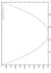
Figure 2: Behaviour of the $\mu(\gamma)$ function, for $\gamma\in[0,1]$, with $q=2$.

Only $\mu_{1}$ is positive and thus we must have $\mu>\mu_{1}$, i.e.

$$(1-\gamma)^{2}+\frac{\gamma^{2}}{q-1}>\mu_{1}.$$ (15)

Again, we have two roots for the equation $(1-\gamma)^{2}+\frac{\gamma^{2}}{q-1}=\mu_{1}$, namely:

$$\gamma_{0} =\frac{q-1}{q}\left(1-\sqrt{1-\frac{q}{q-1}(1-\mu_{1}})\right)$$ (16)

$$\gamma_{1} =\frac{q-1}{q}\left((1+\sqrt{1+\frac{q}{q-1}(1-\mu_{1}})\right).$$ (17)

Only $\gamma_{0}<\frac{q-1}{q}$, and thus we must have

$$\gamma <\gamma_{0}=\frac{q-1}{q}(1-\sqrt{1-\frac{q}{q-1}(1-\mu_{1}}).$$ (18)

Then, when $s\rightarrow\infty$, we have $\mu_{1}\rightarrow R^{\prime}$, and we get

$$\gamma <\tau=\frac{q-1}{q}\left(1-\sqrt{1-\frac{q}{q-1}(1-R^{\prime})}\right)$$ (19)

Using the fact that $k_{GRS}-1=n-d_{GRS}$, i.e $R^{\prime}=1-\delta_{GRS}$, we get

$$\tau=\frac{q-1}{q}\left(1-\sqrt{1-\frac{q}{q-1}\delta_{GRS}}\right),$$

which the $q$-ary Johnson radius. ∎

The previous Proposition proves that this method enables to list-decode any alternant code up to the $q$-ary Johnson bound. This bound is better than the error correction capacities of the previous algorithms [GS99, Ber08]. For the binary case, we plot in Figure 3 the binary Johnson bound (weighted multiplicities, this paper), the generic Johnson bound (straight Guruswami-Sudan, or Bernstein), and the unambiguous decoding bound (Patterson). As usually, the higher the normalised minimum distance is, the better the Johnson bound is.

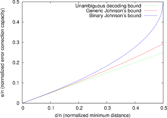
Figure 3: Comparison of the relative error capacities of different decoding algorithm for binary alternant codes — This applies to binary square-free Goppa codes.

5.2 Complexity Analysis

The main issue is to give explicitly how large the “order of multiplicity” $s$ has to be, to approach closely the limit correction radius, $\tau(\delta_{GRS})$ as given by (12).

Lemma 5.6.

To list-decode up to a relative radius of $\gamma=(1-\varepsilon)\tau$, it is enough to have an auxiliary multiplicity $s$ of size $\mathcal{O}(\frac{1}{\varepsilon})$, where the constant in the big-$\mathcal{O}$ depends only on $q$ and on the pseudo-rate $R^{\prime}=\frac{k_{GRS}-1}{n}$ of the GRS code.

Proof.

To get the dependency on $s$, we work out Equation (18). Let us denote by $\gamma(s)$ the achievable relative correction radius for a given $s$. We have

$$\gamma(s) =\frac{q-1}{q}\left(1-\sqrt{1-\frac{q}{q-1}\left(1-\mu_{1}(s)\right)}\right),$$ (20)

with $\mu_{1}(s)=\frac{R^{\prime}+\sqrt{R^{\prime 2}+4\frac{R^{\prime}}{s}}}{2}$. We use that $\sqrt{1+x}<1+\frac{x}{2}$, for all $x>0$. First, we have the bound:

$$\mu_{1}(s) =\frac{R^{\prime}+\sqrt{R^{\prime 2}+4\frac{R^{\prime}}{s}}}{2}$$ (21)

$$=\frac{R^{\prime}}{2}\left(1+\sqrt{1+\frac{4}{sR^{\prime}}}\right)$$ (22)

$$\leq\frac{R^{\prime}}{2}\left(1+\left(1+\frac{4}{2sR^{\prime}}\right)\right)$$ (23)

$$=R^{\prime}+\frac{1}{s}.$$ (24)

Now, calling $K_{q}(R^{\prime})$ the quantity $1-\frac{q}{q-1}(1-R^{\prime})$, we compute:

$$\gamma(s) =\frac{q-1}{q}\left(1-\sqrt{1-\frac{q}{q-1}\left(1-\mu_{1}(s)\right)}\right)$$ (25)

$$\geq\frac{q-1}{q}\left(1-\sqrt{1-\frac{q}{q-1}\left(1-R^{\prime}-\frac{1}{s}\right)}\right)$$ (26)

$$=\frac{q-1}{q}\left(1-\sqrt{K_{q}(R^{\prime})+\frac{q}{q-1}\frac{1}{s}}\right)$$ (27)

$$=\frac{q-1}{q}\left(1-\sqrt{K_{q}(R^{\prime})\left(1+\frac{q}{q-1}\frac{1}{s}\frac{1}{K_{q}(R^{\prime})}\right)}\right)$$ (28)

$$\geq\frac{q-1}{q}\left(1-\sqrt{K_{q}(R^{\prime})}\left(1+\frac{1}{2}\frac{q}{q-1}\frac{1}{s}\frac{1}{K_{q}(R^{\prime})}\right)\right)$$ (29)

$$=\frac{q-1}{q}\left(1-\sqrt{K_{q}(R^{\prime})}-\sqrt{K_{q}(R^{\prime})}\frac{1}{2}\frac{q}{q-1}\frac{1}{s}\frac{1}{K_{q}(R^{\prime})}\right)$$ (30)

$$=\frac{q-1}{q}\left(1-\sqrt{K_{q}(R^{\prime})}\right)-\frac{1}{2}\frac{1}{s\sqrt{K_{q}(R^{\prime})}}$$ (31)

$$=\tau-\frac{1}{2s\sqrt{K_{q}(R^{\prime})}}$$ (32)

$$=\tau\left(1-\frac{1}{2s\tau\sqrt{K_{q}(R^{\prime})}}\right)$$ (33)

Thus, to reach a relative radius $\gamma=(1-\varepsilon)\tau$, it is enough to take

$$s=\frac{1}{2\varepsilon\tau\sqrt{K_{q}(R^{\prime})}}=\mathcal{O}(\frac{1}{\varepsilon}).$$ (34)

∎

The most expensive computational step in these kinds of list-decoding algorithms is the interpolation step, while root-finding is surprisingly cheaper [AP00, RR00]. This is the reason why we focus on the complexity of this step. We assume the use of the so-called Koetter algorithm [Köt96] (see for instance [Tri10, KMV10] for a recent exposition), to compute the complexity of our method. It is in general admitted that this algorithm, which also may help in various interpolation problems, has complexity $\mathcal{O}(lC^{2})$, where $l$ is the $Y$-degree of the $Q(X,Y)$ polynomial, and $C$ is the number of linear equations given by the interpolation constraints. It can be seen as an instance of the Buchberger-Möller problem [MB82].

Corollary 5.7.

The proposed list-decoding runs in

$$\mathcal{O}(\frac{1}{\varepsilon^{-5}}n^{2})$$ (35)

field operations to list-decode up to $(1-\varepsilon)\tau\cdot n$ errors, where the constant in the big-$\mathcal{O}$ depends only on $q$ and the pseudo-rate $R^{\prime}$.

Proof.

Assume that we would like to decode up to $n\gamma=n(1-\varepsilon)\tau$. The number of equations given by the interpolation conditions can be seen to be $\mathcal{O}(ns^{2})$ (see Equation (13)). Now, the list size $\ell$ is bounded above by the $Y$-degree of the interpolation polynomial $Q(X,Y)$, which is at most

$$\frac{sn((1-\gamma)^{2}+\frac{\gamma^{2}}{q-1})}{k-1}=\mathcal{O}(s),$$ (36)

for fixed $R^{\prime}=\frac{k-1}{n}$. Fitting $s=\mathcal{O}(\frac{1}{\varepsilon})$, we conclude that this method runs in $\mathcal{O}(n^{2}\varepsilon^{-5})$.

Regarding the Root-Finding step, one can use [RR00], where an algorithm of complexity $\mathcal{O}(\ell^{3}k^{2})$ is proposed, assuming $q$ is small. Indeed, classical bivariate factorisation or root finding algorithms rely on a univariate root-finding step, which is not deterministic polynomially in the size of its input, when $q$ grows. But our interest is for small $q$, i.e. 2 or 3, and we get $\mathcal{O}(s^{3}n^{2})$, which is less than the cost of the interpolation step. ∎

Corollary 5.8.

To reach the non relative $q$-ary Johnson radius:

$$\left\lceil\frac{q-1}{q}n\left(1-\sqrt{1-\frac{q}{q-1}\frac{d_{GRS}}{n}}\right)-1\right\rceil,$$

it is enough to have $s=\mathcal{O}(\frac{1}{n})$. Then, the number of field operations, is

$$\mathcal{O}(n^{7}),$$

where the constant in the big-$\mathcal{O}$ only depends on $q$ and $R^{\prime}$.

Proof.

It is enough to consider that

$$\left\lceil\frac{q-1}{q}n\left(1-\sqrt{1-\frac{q}{q-1}\frac{d_{GRS}}{n}}\right)-1\right\rceil=n\tau(1-\varepsilon),$$

with $\varepsilon=\mathcal{O}(\frac{1}{n})$. ∎

5.3 Application to classical binary Goppa codes

The most obvious application of this algorithm is the binary Goppa codes defined with a square-free polynomial $G$ (we do not detail the result for the general $q$-ary case, which is less relevant in practice). Indeed, since we have

$$\Gamma_{2}(L,G)=\Gamma_{2}(L,G^{2}),$$

both codes benefit at least from the dimension of $\Gamma_{2}(L,G)$ and the distance of $\Gamma_{2}(L,G^{2})$. Thus, if $\deg G=t$, we have the decoding radii given in Table 1. In addition, we compare in Table 2 the different decoding radii for practical values.

Generic list-decoding	Bernstein	Binary list-decoding
$\left\lceil n-\sqrt{n(n-2t)}\right\rceil-1$	$n-\sqrt{n(n-2t-2)}$	$\left\lceil\frac{1}{2}\left(n-\sqrt{n(n-4t-2}\right)\right\rceil-1$

Table 1: Comparison of the claimed decoding radii in terms of $t$, the degree of the square-free polynomial $G(X)$ using to construct the Goppa code.

Algorithm 2 List-decoding of binary Goppa codes

0:   $L=(\alpha_{1},\dots,\alpha_{n})$ A Goppa polynomial $G$, square-freeThe corresponding Goppa code $C=\Gamma_{2}(L,G)$ The associated evaluation map $\operatorname{ev}$The relative decoding radius $\gamma=(1-\varepsilon)\tau$The received word $y\in\mathbb{F}_{q}^{n}$

1:   View $\Gamma_{2}(L,G)$ as $\Gamma_{2}(L,G^{2})$

2:   Consider the Generalised Reed-Solomon code $GRS_{q^{m}}(L,B,k)$ above $\Gamma_{2}(L,G^{2})$

3:   Use Algorithm 1 to find all the codewords at distance $\gamma n$ of $y$

$n$	$k$	$t$	Guruswami-Sudan	Bernstein	Binary list-decoding
16	4	3	4	4	5
32	2	6	7	8	9
64	16	8	9	9	10
64	4	10	11	12	13
128	23	15	16	17	18
128	2	18	20	20	22
256	48	26	28	28	30
256	8	31	33	34	36
512	197	35	36	37	38
512	107	45	47	48	50
512	17	55	58	59	63
1024	524	50	51	52	53
1024	424	60	62	62	74
1024	324	70	73	73	76
1024	224	80	83	84	88
1024	124	90	94	95	100
2048	948	100	103	103	105
2048	728	120	124	124	128
2048	508	140	145	146	151
2048	398	150	156	157	163
2048	288	160	167	167	175
2048	178	170	178	178	187

Table 2: Comparison of the error capacities of different decoding algorithms for square-free binary Goppa codes, with respect to the length $n$, the dimension $k$, and the degree $t$ of $G(X)$.

Appendix A The number of unknowns

Proposition A.1.

Let $Q(X,Y)\in\mathbb{F}[X,Y]$ be a bivariate polynomial such that $\operatorname{wdeg}_{1,k-1}Q(X,Y)<D$. Then, the number $N_{k-1,D}$ of nonzero coefficients of $Q(X,Y)$ is larger than or equal to

$$\frac{D^{2}}{2(k-1)}\cdot$$ (37)

Proof.

Let us write

$$Q(X,Y)=\sum_{i=0}^{\ell}Q_{i}Y^{i},$$

with $\deg Q_{j}(X)<D-(k-1)j$, and $\ell$ maximal such that $(k-1)\ell<D$. Then

$$N_{k-1,D}= \sum_{i=0}^{\ell}\left(D-(k-1)i\right)$$ (38)

$$= (\ell+1)D-(k-1)\frac{\ell(\ell+1)}{2}$$ (39)

$$= (\ell+1)\left(D-(k-1)\frac{l}{2}\right)$$ (40)

$$> (\ell+1)\left(D-\frac{D}{2}\right)$$ (41)

$$= (\ell+1)\frac{D}{2}$$ (42)

$$\geq \frac{D^{2}}{2(k-1)}\cdot$$ (43)

∎

Appendix B The number of interpolation constraints

The following proposition can be found in any book of computer algebra, for instance [CLO92].

Proposition B.1.

Let $Q(X,Y)\in\mathbb{F}[X,Y]$ be a bivariate polynomial. The number of terms of degree at most $s$ in $Q(X,Y)$ is $\binom{s+1}{2}$.

Corollary B.2.

The condition $\operatorname{mult}(Q(X,Y)),(a,b))\geq s$ imposes $\binom{s+1}{2}$ linear equations on the coefficients of $Q(X,Y)$. Let $(a_{i},b_{i})\in\mathbb{F}^{2}$ be points and $s_{i}\in{\mathbb{N}}$ be multiplicities, $i\in[1,n]$. Then the number of linear equations imposed by the conditions

$$\operatorname{mult}(Q(X,Y),(a_{i},b_{i}))\geq s_{i},\quad i\in[1,n],$$ (44)

is

$$\sum_{i=1}^{n}\binom{s_{i}+1}{2}.$$ (45)

References

- [AP00] Daniel Augot and Lancelot Pecquet. A Hensel lifting to replace factorization in list decoding of algebraic-geometric and Reed-Solomon codes. IEEE Transactions on Information Theory, 46(7):2605–2613, 2000.
- [Ber68] Elwyn R. Berlekamp. Algebraic coding theory. McGraw-Hill, 1968.
- [Ber84] Elwyn R. Berlekamp. Algebraic Coding Theory, Revised 1984 Edition. Aegean Park Press, 1984.
- [Ber08] Daniel J. Bernstein. List decoding for binary Goppa codes. http://cr.yp.to/codes/goppalist-20081107.pdf, 2008.
- [BLP10] Daniel J. Bernstein, Tanja Lange, and Christiane Peters. Wild McEliece. Cryptology ePrint Archive, Report 2010/410, 2010.
- [CLO92] David Cox, John Little, and Donald O’Shea. Ideals, Varieties and Algorithms. Springer, 1992.
- [Eli91] Peter Elias. Error-correcting codes for list decoding. IEEE Transactions on Information Theory, 37(1):5–12, 1991.
- [Ful89] William Fulton. Algebraic curves. Advanced Book Classics. Addison-Wesley Publishing Company, Redwood City, CA, 1989.
- [GS99] V. Guruswami and M. Sudan. Improved decoding of Reed-Solomon and algebraic-geometry codes. IEEE Transactions on Information Theory, 45(6):1757 –1767, 1999.
- [Gur04] Venkatesan Guruswami. List Decoding of Error-Correcting Codes - Winning Thesis of the 2002 ACM Doctoral Dissertation Competition, volume 3282 of Lectures Notes in Computer Science. Springer, 2004.
- [Gur07] Venkatesan Guruswami. Algorithmic results in list decoding. Now Publishers Inc, 2007.
- [KMV10] Ralf Koetter, Jun Ma, and Alexander Vardy. The Re-Encoding Transformation in Algebraic List-Decoding of Reed-Solomon Codes, 2010.
- [Köt96] Ralf Kötter. On Algebraic Decoding of Algebraic-Geometric and Cyclic Codes. PhD thesis, University of Linköping, 1996.
- [KV03] Ralf Kötter and Alexander Vardy. Algebraic soft-decision decoding of Reed-Solomon codes. IEEE Transactions on Information Theory, 49(11):2809–2825, 2003.
- [MB82] H. Michael Möller and Bruno Buchberger. The construction of multivariate polynomials with preassigned zeros. In Proceedings of the European Computer Algebra Conference on Computer Algebra, EUROCAM’82, pages 24–31, London, UK, 1982. Springer-Verlag.
- [MS83] F. J. Macwilliams and N. J. A. Sloane. The Theory of Error-Correcting Codes. North-Holland Mathematical Library. North Holland, 1983.
- [Pat75] N. Patterson. The algebraic decoding of Goppa codes. IEEE Transactions on Information Theory, 21(2):203–207, 1975.
- [Rot06] Ron Roth. Introduction to Coding Theory. Cambridge University Press, 2006.
- [RR00] R. M. Roth and G. Ruckenstein. Efficient decoding of Reed-Solomon codes beyond half the minimum distance. IEEE Transactions on Information Theory, 46(1):246–257, 2000.
- [Sti93] Henning Stichtenoth. Algebraic function fields and codes. Universitext. Springer-Verlag, Berlin, 1993.
- [Sud97] Madhu Sudan. Decoding of Reed-Solomon codes beyond the error-correction bound. Journal of Complexity, 13(1):180 – 193, 1997.
- [TR03] Ido Tal and Ronny M Roth. On list decoding of alternant codes in the Hamming and Lee metrics. In Proceedings of IEEE International Symposium on Information Theory, page 364, 2003.
- [Tri10] Peter V. Trifonov. Efficient Interpolation in the Guruswami-Sudan Algorithm. IEEE Transactions on Information Theory, 56(9):4341–4349, 2010.
- [VK00] Alexander Vardy and Ralf Koetter. Algebraic Soft-Decision Decoding of Reed-Solomon Codes. 53 pages, circulated before the IEEE publication, 2000.
- [VNT07] Serge Vlăduţ, Dmitry Nogin, and Michael Tsfasman. Algebraic Geometric Codes: Basic Notions. American Mathematical Society, Boston, MA, USA, 2007.
- [Wu08] Y. Wu. New list decoding algorithms for Reed-Solomon and BCH codes. IEEE Transactions on Information Theory, 54(8):3611–3630, 2008.