The frustrated spherical model: an alternative to Ginzburg-Landau Hamiltonians with competing interactions

Abstract

We solve analytically the Langevin dynamics of the classic spherical model considering the ferromagnetic exchange and a long-range antiferromagnetic interaction. Our results in the asymptotic regime, shows an equivalence in the functionality of the spatial and self-correlations between this model and the recently studied Ginzburg-Landau frustrated model within the Hartree approximation. A careful discussion is done about the low temperature behavior in the context of glassy dynamics. The appearance of interesting features regarding the establishment of the ferromagnetic phase is also analyzed in view of the effects of the spherical restriction. We propose a new variant of the spherical model in which the global restriction is substituted by an infinite set of restrictions over finite size regions. This modification leads to a new dynamical equation that suggests the appearance of the low temperature phase transition even in the non-frustrated case were the classic spherical model fails.

I Introduction

The study of the fundamental role of microscopic interactions on the relevant properties of magnetic materials involves two main approaches: discrete models, like the Ising model which is commonly used to represent systems with uniaxial anisotropy, and continuous models among which the Ginzburg-Landau model is one of the most widely known. These two approaches have been extensively used both numericallyGleiser et al. (2003); Jagla (2004); Nicolao and Stariolo (2007); Díaz-Méndez and Mulet (2010) and analyticallyGarel and Doniach (1982); Roland and Desai (1990); Pighín and Cannas (2003); Mulet and Stariolo (2007) to describe equilibrium and dynamical features observed in real systems.Rosensweig et al. (1983); Seul and Wolfe (1992); Seul and Andelman (1995); Saratz et al. (2010a) Concerning to the local magnetization bound, unlike the Ising model in which the site magnetization take values $\pm 1$, the Ginzburg-Landau double well potential is the responsible to guaranty the non-divergence of the local magnetization. Unfortunately, this potential introduce a strong non-linearity in the dynamical equations describing the time evolution of the local order parameter, and do not allow the magnetization of the system to saturate at high enough external fields. On the other hand, for discrete models some dynamical treatments are forbidden due to the natural impossibility of define temporal derivatives of the local magnetization.

In this context, the spherical modelBerlin and Kac (1952); Baxter (1982) is something in between. It is a linear model that can be treated analytically, while the saturation of the magnetization is guarantied by means of the spherical constraint. Despite this niceties, this model fails in obtaining of the ferromagnetic transition in two dimensions. On the basis of this disagreement it has been argued that the spherical constrain allows the system to be in a large number of disordered configurations. In two dimensions this degeneracy prevents the system to reach a ferromagnetic phase transition at any non-zero temperature. To manage this difficulty a lot of work have been carried out making some radical modifications as, for example, the substitution of the short range exchange interactions by a long range ferromagnetic one.Brody (1994); Cannas et al. (2000)

Recently, a great effort has been done in the study of the system with competing isotropic interactions, i. e. systems whose fluctuation spectrum has a minimum in a non-zero radius spherical shell in the inverse space.Grousson et al. (2000, 2002); Prozorov et al. (2008); Tarzia and Coniglio (2006); Díaz-Méndez et al. (2010) In magnetic systems, these interaction are usually represented by the ferromagnetic exchange interaction and the anti-ferromagnetic long-ranged dipolar interaction. The Langevin dynamic of a Ginzburg-Landau Hamiltonian with such interactions have been studied previously by means of the Hartree self-consistent field approximation.Mulet and Stariolo (2007); Díaz-Méndez et al. (2010) In these works the authors confirm the theoretical picture found analytically by means of numerical simulations. Moreover, the symmetry breaking properties of the model were also studied by means of a very similar procedure.Mendoza-Coto et al. (2010) In particular, it was shown that taking the infinite time limit it was possible to encounter the phase transition to the modulated ordered state by means of purely dynamical calculations.

In the present work we solve the Langevin dynamics of the spherical model considering the common square field-gradient attractive term plus a repulsive long-range antiferromagnetic term in the long times limit. We show that, starting from a disordered initial condition, quenches to the $T=0$ regime develops a long time dynamics very close to that encountered in Ref. Díaz-Méndez et al. (2010). As it is expected, for this frustrated spherical model, the value of the critical field dividing the two different dynamical regimes is also the saturation value. For $T>0$ we found a standard paramagnetic relaxation after certain characteristic time. Anyway, the divergence of this time for low temperatures as well as the existence of modulated domains of typical length can be related to the reminiscence of a glassy region not completely verified for our model. The monotony of the $h$-$T$ curve for a fixed magnetization is also an interesting finding that connects the results with recent experimental works. Finally, we propose a new variant of the spherical model in which the global restriction is substituted by an infinite set of restrictions over finite spatial regions of the system. This lead to a new dynamical equation that is also presented in detail. We discuss the way in which this modification suggest the appearance of the low temperature phase transition even in the non-frustrated case were the spherical model fails.

The rest of the paper is organized as follows. The next section is completely devoted to the presentation of the formalism and the solution of the dynamical equation for all the regimes involving the value of the applied external field. Some commonly studied observables as spatial and self-correlations are presented and discussed in some detail in section III comparing its asymptotic expressions with those recently obtained for the Ginzburg-Landau model. In section IV the more relevant findings are discussed in the light of the known phenomenology of related models and some experimental observations, in order to better understand the advantages of using the spherical model in the context of competitive interactions. Also a new dynamical equation is obtained by means of suitable modifications to the standard model and is discussed the way in which this new approach may lead to the appearance of the phase transition. We summarize the most important results and discussions in section V. In appendix A the spatial correlations of some particular configurations are calculated by means of geometrical considerations.

II Model and Formalism

We consider the following Hamiltonian dependent on the local parameter $\phi(\vec{x},t)$

$${\cal H}[\phi(\vec{x})] = \frac{1}{2}\int_{\Omega}d^{d}x\left[(\vec{\nabla}\phi)^{2}-2h\phi(\vec{x})\right]$$ (1)

$$- \frac{1}{2\delta}\int_{\Omega}\int_{\Omega}d^{d}x\ d^{d}x^{\prime}J(\vec{x}-\vec{x}^{\prime})\ \phi(\vec{x})\ \phi(\vec{x}^{\prime})$$

where $J(\vec{x}-\vec{x}^{\prime})$ represents a repulsive, isotropic, competing interaction and $\Omega$ is the $d$-dimensional volume of the system, which is finally taken as infinity. The homogeneous external field is represented by $h$ and the parameter $\delta$ measures the relative intensity between the attractive and repulsive interactions. The local field is subjected to the restriction

$$\int_{\Omega}\phi^{2}(\vec{x})\ d^{d}x=m^{2}\Omega$$ (2)

that represents a system with local magnetization $m$. In order to include this restriction in the dynamics it is widely used the effective HamiltonianCugliandolo and Dean (1995)

$${\cal H}^{\prime}[\phi(\vec{x})]={\cal H}[\phi(\vec{x})]+\frac{\lambda(t)}{2}\left[\int_{\Omega}\phi^{2}(\vec{x})d^{d}x-m^{2}\Omega\right]$$ (3)

and in consequence the Langevin equation of motion is given by

$$\frac{\partial\phi(\vec{x},t)}{\partial t} = \nabla^{2}\phi(\vec{x})-\frac{1}{\delta}\int_{\Omega}d^{d}x^{\prime}J(\vec{x}-\vec{x}^{\prime})\phi(\vec{x}^{\prime})$$ (4)

$$+ h-\lambda(t)\phi(\vec{x})+\eta(\vec{x},t)$$

the solution of this equation is carried out in the inverse space, defined by the following Fourier transforms

$$\phi(\vec{x}) = \int\frac{d^{d}k}{(2\pi)^{d}}e^{i\vec{k}\cdot\vec{x}}\hat{\phi}(\vec{k})$$

$$\hat{\phi}(\vec{k}) = \int d^{d}x\ e^{-i\vec{k}\cdot\vec{x}}\phi(\vec{x})$$ (5)

The equation of motion in the momenta space is given by

$$\frac{\partial\phi(\vec{k},t)}{\partial t} = -\left[k^{2}+\frac{1}{\delta}J(k)+\lambda(t)\right]\phi(\vec{k},t)$$ (6)

$$+ h(\vec{k})+\eta(\vec{k},t)$$

and its solution can be written in terms of the response function $R(\vec{k},t,t^{\prime})$ as

$$\phi(\vec{k},t) = \phi(\vec{k},0)R(\vec{k},t,0)+\int_{0}^{t}R(\vec{k},t,t^{\prime})\eta(\vec{k},t^{\prime})dt^{\prime}$$ (7)

$$+ \int_{0}^{t}R(\vec{k},t,t^{\prime})h(\vec{k})dt^{\prime}$$

where

$$R(\vec{k},t,t^{\prime})=\frac{Y(t^{\prime})}{Y(t)}e^{-\hat{A}(k)(t-t^{\prime})}$$ (8)

It has been also defined $\hat{A}(k)=A(k)-A(k_{0})$, $Y(t)=e^{\int_{0}^{t}I(t^{\prime})dt^{\prime}}$, $I(t)=A(k_{0})+\lambda(t)$ and $A(k)=k^{2}+\frac{1}{\delta}J(k)$. At this point the problem has been formally solved, except for the fact that the parameter $\lambda(t)$ remains unknown. It can be shown that the spherical restriction leads to the normalization condition $C(t,t)=m^{2}$, where $C(t,t^{\prime})$ represents the self-correlation function, obtained from the usual correlation function given by

$$C(\vec{k},\vec{k}^{\prime},t,t^{\prime})=\langle\phi(\vec{k},t)\phi(\vec{k}^{\prime},t^{\prime})\rangle$$ (9)

Thus, to impose the normalization condition for the self-correlation function allows to obtain the following equation

$$m^{2}K(t) = \Delta f(t)+2T\int_{0}^{t}K(\tau)f(t-\tau)d\tau$$ (10)

$$+ h^{2}\left[\int_{0}^{t}K^{1/2}(\tau)e^{-\hat{A}(0)(t-\tau)}d\tau\right]^{2}$$

where $K(t)=Y(t)^{\frac{1}{2}}$ and

$$f(t)=\frac{1}{(2\pi)^{d}}\int d^{d}k\ e^{-2\hat{A}(k)t}$$ (11)

In systems with isotropic competing interactions the fluctuation spectrum $\hat{A}(k)$ has a minimum in a shell in the inverse space of certain radius $k_{0}$. As it was shown in previous worksMulet and Stariolo (2007); Díaz-Méndez et al. (2010) the long time behavior of $f(t)$ is dominated by the local topology of the fluctuation spectrum around $k_{0}$. In consequence, it is enough to consider an expansion of the fluctuation spectrum $\hat{A}(k)$ up to second order around its minimum, such expansion has the form

$$\hat{A}(k)=\frac{A_{2}}{2}(k-k_{0})^{2}$$ (12)

where $A_{2}=\frac{d^{2}\hat{A}(k)}{dk^{2}}$. With these ingredients it is straight forward to obtain the following asymptotic result

$$f(t)=\frac{C}{t^{1/2}}$$ (13)

where $C$ is certain uninteresting constant depending on system dimension. At this point we carry out the solution of the problem separately, first we analyze the zero temperature case and then the non-zero temperature case.

II.1 Case $T=0$

In order to solve equation (10) at zero temperature, we found suitable to define the function

$$S(t)=\int_{0}^{t}K^{1/2}(\tau)e^{-\hat{A}(0)(t-\tau)}d\tau$$ (14)

and then to split up the original equation into the following set of equations

$$m^{2}K(t) = \Delta f(t)+h^{2}S^{2}(t)$$

$$\frac{dS(t)}{dt} = -\hat{A}(0)S(t)+K(t)^{\frac{1}{2}}$$ (15)

with the initial conditions $K(0)=1$ and $S(0)=0$. Note that this system can be put in the form

$$\frac{dS(t)}{dt}=-\hat{A}(0)S(t)+\frac{1}{m}\left(\Delta f(t)+h^{2}S^{2}(t)\right)^{\frac{1}{2}}$$ (16)

So, we have to find the asymptotic solution of the above differential equation. In order to do this we compare the terms $f(t)$ and $S^{2}(t)$. In general we can see that there are several possibilities varying $h$. For small fields $f(t)$ dominates the dynamics and in consequence $S^{2}(t)\propto f(t)$. On the other hand, fields higher than certain critical value $h_{c}$ leads to a different behavior. In what follows we obtain the different solutions for $S(t)$ and $K(t)$ varying the external field $h$.

II.1.1 $h<h_{c}$

In the case of small enough fields we can obtain that $S^{2}(t)=\lambda f(t)$. This consideration implies the relation

$$\frac{1}{m}\left(\Delta f(t)+h^{2}S^{2}(t)\right)^{\frac{1}{2}}=\frac{1}{m}\left(\Delta+h^{2}\lambda\right)^{\frac{1}{2}}f(t)^{\frac{1}{2}}$$ (17)

This leads to the simplified equation

$$\frac{dS(t)}{dt}=-\hat{A}(0)S(t)+\frac{1}{m}\left(\Delta+h^{2}\lambda\right)^{\frac{1}{2}}f(t)^{\frac{1}{2}}$$ (18)

whose asymptotic solution is given by

$$S(t)=\frac{1}{m\hat{A}(0)}\left(\Delta+h^{2}\lambda\right)^{\frac{1}{2}}f(t)^{\frac{1}{2}}$$ (19)

At this point to consider the proposed ansatz implies that

$$\lambda=\frac{\Delta}{m^{2}\hat{A}(0)^{2}-h^{2}}$$ (20)

and

$$K(t)=\lambda\hat{A}(0)^{2}f(t)$$ (21)

It is worth to note that from the definition of $\lambda$ one can see the existence of a critical field $h_{c}=m\hat{A}(0)$.

II.1.2 $h=h_{c}$

We start by writing equation (16) in the form

$$\frac{dS(t)}{dt}=-\hat{A}(0)S(t)+\frac{hS(t)}{m}\left(1+\frac{\Delta f(t)}{h^{2}S^{2}(t)}\right)^{\frac{1}{2}}$$ (22)

In the long time limit $\Delta f(t)\ll h^{2}S^{2}(t)$, then it is possible to write

$$\frac{dS(t)}{dt}=-\hat{A}(0)S(t)+\frac{hS(t)}{m}\left(1+\frac{\Delta f(t)}{2h^{2}S^{2}(t)}\right)$$ (23)

considering an expansion up to first order of the non-linear contribution. Note that if we take now $h=h_{c}=m\hat{A}(0)$, the first order contribution of the non-linear term cancels and we have

$$\frac{dS(t)}{dt}=\frac{\Delta}{m^{2}\hat{A}(0)}\frac{f(t)}{2S(t)}$$ (24)

whose solution yields

$$S^{2}(t)=\frac{\Delta}{m^{2}\hat{A}(0)}\int^{t}f(\tau)d\tau$$ (25)

and

$$K(t)=\frac{\Delta\hat{A}(0)}{m^{2}}\int^{t}f(\tau)d\tau$$ (26)

Expressions (25) and (26) has no lower integration limit. This is related with the fact that, in the long time limit, any constant can be neglected in comparison with the increasing functions $S(t)$ and $K(t)$.

II.1.3 $h>h_{c}$

In this case, from equation (16) in the long time regime, it is fairly easy to see that

$$S(t)\propto e^{\left(-\hat{A}(0)+\frac{h}{m}\right)t}$$ (27)

and in consequence

$$K(t)\propto e^{2\left(-\hat{A}(0)+\frac{h}{m}\right)t}$$ (28)

II.2 Case $T>0$

At finite temperature the equation (10) contains a convolution term with the function $f(t)$, which leads always to a exponential long time behavior, as have been obtain previously in literature. In order to clarify this point, we propose the ansatzDíaz-Méndez et al. (2010)

$$S(t)=\int_{0}^{t}K^{1/2}(\tau)e^{-\hat{A}(0)(t-\tau)}d\tau=\xi K^{\frac{1}{2}}(t)$$ (29)

for the asymptotic dynamic. By doing this, equation (10) turns in an integral equation whose solution can be found by means of the Laplace transform. Using expression (13) for $f(t)$ we get

$$K(t)\propto e^{b^{2}t}$$ (30)

where $b$ and $\xi$ are the solutions of the following system of equations

$$b=\frac{2TC\Gamma(\frac{1}{2})}{m^{2}-h^{2}\xi^{2}}\ ,\ \ \ \ \ \ \ \ \xi=\frac{2}{b^{2}+2\hat{A}(0)}$$ (31)

Finally, it is worth to note that the above system of equations always give rise to positive values for both, $b$ and $\xi$. This means that at any finite temperature the model reaches the same asymptotic dynamics.

III Observables

At this point we have been able to find the asymptotic behavior of the function $K(t)$ for any value of temperature and external field. This allows the calculation of some commonly studied statistical observables. In particular, we obtain in this section the mean value of the local field $\phi$ (magnetization), the self-correlation function and the spatial correlation function. For some of these magnitudes closed expressions are found in terms of the function $K(t)$.

III.1 Mean value

Starting from expression (7) we obtain the following expression for the mean value

$$\left\langle\phi\right\rangle=h\ \xi(h,T)$$ (32)

where

$$\xi(h,T)=\lim_{t\rightarrow\infty}\frac{S(t)}{K(t)^{\frac{1}{2}}}$$ (33)

This expression implies that at $T=0$

$$\langle\phi\rangle=\left\{\begin{array}[]{ll}\frac{h}{\hat{A}(0)}&\textrm{for $h<h_{c}$}\\ \\ m&\textrm{for $h\geq h_{c}$}\\ \end{array}\right.$$ (34)

while for any finite temperature $\xi(h,T)$ is given by the solution of the system (31). In order to clarify such a dependency of the mean value with the external field and temperature we define the following non-dimensional magnitudes

$$\frac{h}{h_{c}}\rightarrow{h},\ \ \ \ \frac{C\Gamma(\frac{1}{2})T}{\hat{A}(0)^{\frac{1}{2}}m^{2}}\rightarrow{T},\ \ \ \ \frac{\left\langle\phi\right\rangle}{m}\rightarrow{\phi}$$ (35)

which are the variables uses in the figure 1.

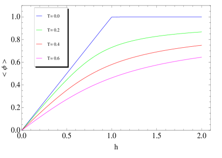
Figure 1: Dependence of the mean value of the local field $\langle\phi\rangle$ with the external field $h$ for several temperatures.

As can be seen from figure 1, at zero temperature and $h<h_{c}$ the system behaves like a purely paramagnetic material with a completely linear relation between magnetization and external field. On the other hand, for any finite temperature the relation between the mean value and the external field is no longer linear in such a way that $\langle\phi\rangle$ is always an increasing function of the applied external field.

III.2 Self-correlation function

In order to look inside the ordering process we calculate now the self-correlation function, defined as $C(t,t^{\prime})=\left\langle\phi(\vec{r},t)\phi(\vec{r},t^{\prime})\right\rangle-\left\langle\phi(\vec{r},t)\right\rangle\left\langle\phi(\vec{r},t^{\prime})\right\rangle$. In terms of the function $K(t)$ this magnitude can be written

$$C(t,t^{\prime}) = \frac{\Delta}{\sqrt{K(t)K(t^{\prime})}}f\left(\frac{t+t^{\prime}}{2}\right)$$

$$+ \frac{2T}{\sqrt{K(t)K(t^{\prime})}}\int_{0}^{t^{\prime}}K(\tau)f\left(\frac{t+t^{\prime}}{2}-\tau\right)d\tau$$

In this way at $T=0$ we obtain

$$C(t,t^{\prime})\propto\left\{\begin{array}[]{ll}\frac{(4tt^{\prime})^{\frac{1}{4}}}{(t+t^{\prime})^{\frac{1}{2}}}&\textrm{for $h<h_{c}$}\\ \\ \frac{1}{\left(t+t^{\prime}\right)^{\frac{1}{2}}(4tt^{\prime})^{\frac{1}{4}}}&\textrm{for $h=h_{c}$}\\ \\ \frac{e^{-(\hat{A}(0)+\frac{h}{m})(t+t^{\prime})}}{\left(t+t^{\prime}\right)^{\frac{1}{2}}}&\textrm{for $h>h_{c}$}\\ \end{array}\right.$$ (36)

Considering our definition of $C(t,t^{\prime})$, it can be seen that for high enough fields ($h\geq h_{c}$) the system presents an interrupted aging and eventually evolves to a ferromagnetic configuration in which there are no fluctuations at all. On the other hand, for $h<h_{c}$ the system shows a slow relaxation typical of a coarsening scenario.

For $T>0$ the long time behavior $(b^{2}t^{\prime}\gg 1)$ of the self-correlations is given by

$$C(t,t^{\prime})=2T\int_{\frac{t-t^{\prime}}{2}}^{\frac{t+t^{\prime}}{2}}f(\tau)e^{-b^{2}\tau}d\tau$$ (37)

showing an interrupted aging and an asymptotic temporal translational invariant relaxation $C(t,t^{\prime})=C(t-t^{\prime})$ typical of systems in thermal equilibrium. This means that for any finite temperature the system always reach the equilibrium state.

III.3 Spatial correlation function

With the aim of study the texture of the system under different conditions, we calculate the spatial correlation function. In our case the isotropy of interactions and initial conditions ensures an homogeneous mean value of the order parameter. The spatial correlation function is defined as $C(R,t)=\langle\phi(\vec{x},t)\phi(\vec{x}+\vec{R},t)\rangle-\langle\phi(\vec{x},t)\rangle\langle\phi(\vec{x}+\vec{R},t)\rangle$. At zero temperature ($T=0$) we obtain

$$C(R,t)=\frac{\Delta}{K(t)}\int\frac{d^{d}\vec{k}}{(2\pi)^{d}}e^{-2\hat{A}(\vec{k})t}e^{i\vec{k}\cdot\vec{R}}$$ (38)

and assuming $k_{0}R\gg 1$ it is possible to obtain

$$C(R,t) \propto \frac{f(t)}{K(t)}\frac{\Delta}{(k_{0}R)^{\frac{d-1}{2}}}$$ (39)

$$\mathrm{cos}\left(k_{0}R-\frac{(d-1)\pi}{4}\right)e^{-\frac{R^{2}}{4A_{2}t}}$$

where $k_{0}$ and $A_{2}$ are defined by the expression (12). At zero temperature the relation $f(t)/K(t)$ contains the dependence with the external field. For $h<h_{c}$ this functionality tends to a constant value, while in the other cases we have

$$\frac{f(t)}{K(t)}\propto\left\{\begin{array}[]{ll}\frac{1}{t}&\textrm{for $h=h_{c}$}\\ \\ \frac{e^{-2\left(-\hat{A}(0)+\frac{h}{m}\right)t}}{t^{\frac{1}{2}}}&\textrm{for $h>h_{c}$}\\ \end{array}\right.$$ (40)

It can be noticed that for fields equal or higher than the critical one the system evolves to the completely ferromagnetic configuration. This can be appreciated in the decay of the spatial correlation function. On the other hand, for $h<h_{c}$ the presence of the exponential term reveals a phenomenology of growing domains with typical length $L(t)\propto t^{\frac{1}{2}}$, very common in models with non-conserved order parameter. These domains represent random oriented modulated structures with frequency $k_{0}$. It is worth to note that the power law decay do not imply the presence of structural defects necessarily, it is possible to show how such a term arise from the average over the ensemble of possible configurations (see Appendix A).

When $T>0$ it is possible to obtain in the equilibrium state

$$C(R) = \lim_{t\rightarrow\infty}2T\int\frac{d^{d}\vec{k}}{(2\pi)^{d}}e^{i\vec{k}\cdot\vec{R}}$$ (41)

$$\int_{0}^{t}d\tau\frac{K(\tau)}{K(t)}e^{-2\hat{A}(\vec{k})(t-\tau)}$$

$$= \frac{2T}{(2\pi)^{d}}\int d^{d}\vec{k}\ \frac{e^{i\vec{k}\cdot\vec{R}}}{b^{2}+A_{2}(k-k_{0})^{2}}$$

where the last integral have been calculated before in Ref. Mulet and Stariolo (2007) and gives

$$C(R)\propto\frac{1}{(k_{0}R)^{\frac{d-1}{2}}}e^{-\frac{R}{\xi}}\mathrm{cos}\left(k_{0}R-\psi\right)$$ (42)

with

$$\xi = \frac{\sqrt{A_{2}}}{b}$$

$$\psi = \frac{(d-1)\pi}{4}-\frac{d-1}{2}\mathrm{tan}^{-1}\left(\frac{1}{k_{0}\xi}\right)$$ (43)

Expression (42) describes a long times state in which a mosaic of modulated structures establishes with a wave length $2\pi/k_{0}$ and a typical dimension equal to the correlation length. As can be seen from (43) this correlation length diverges as temperature tends to zero for $h<h_{c}$, and decreases when the field is augmented. It is worth to note that for $h\geq h_{c}$ the spatial correlation as has been defined tends to zero when $T\rightarrow 0$ indicating an evolution to the homogeneous state.

IV Putting results in context

The results exposed above can also be viewed in the frame of the general scheme currently established in literature. From a static point of view, the infinite time configuration of the system shows no long range stripes order at any finite temperature. This is consistent with the isotropy of our initial conditions and the fact that there is no symmetry breaking. In fact, what we do is to study the long times dynamic of the ensemble of disordered quenches. Anyway, as can be seen in appendix A, the lack of long range order in this case is not due to the ensemble degeneration but to the appearance of randomly oriented domains of typical size.

On the other hand, it has been reported in literatureTarzia and Coniglio (2006, 2007) that below certain temperature the Ginzburg-Landau frustrated system behaves as a typical glass. Even when the spatial correlation found here at finite temperatures (42) is consistent with the glass configuration, the most basic glassy property, that is, the aging behavior of the self-correlations, is not verified in the long times limit. Instead, as we have already pointed, there exists interrupted aging for all non-zero temperature, so the system develops an aging dynamics up to a finite time $\tau_{e}$ that diverges only at $T=0$.

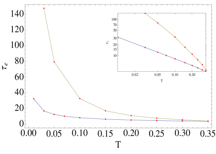
Figure 2: Characteristic time $\tau_{e}$ up to which the aging dynamics can be observed. Upper curve corresponds to a field $h=0.5h_{c}$ and lower curve corresponds to $h=h_{c}$. The inset represents the logarithmic plot of the main figure.

This characteristic time can be obtained by fitting the numerical integration of equation (10) with the asymptotic exponential behavior and is shown as a function of the temperature in figure 2. We can see from the inset that the characteristic time behaves as a power law in a vicinity of $T=0$. As it have been suggested,Godrèche and Luck (2000) this behavior remains very close to that of the glass in the sense that one can always find a temperature below which the aging dynamic establishes up to a time far beyond any laboratory scale.

It is worth to note that the divergence of the correlation length $\xi$ of the ordered domains at $T=0$ have been reported in a number of glassy systems.Tarzia and Coniglio (2007) The spatial correlation (39) certainly accounts for such a glassy configuration. As it is demonstrated in Appendix A, this correlation functionality corresponds to an ensemble of perfect striped configurations every one of which has long range order in a particular direction. This $T=0$ spatial correlations do not show any more the typical exponential decay but a potential decay term $1/R^{(d-1)/2}$ that should not be straightforwardly interpreted as a direct evidence of the presence of topological defects for $d>1$. Correlations obtained by means of the average over the ensemble of perfect modulated structures (i.e. considering all the possible orientations) must be in general a decreasing function of $R$ for $d\geq 2$, even when we have long range order in a particular direction (see Appendix A). For the $T=0$ case the glassy behavior is reinforced from the fact that equilibrium is never reached in any finite time.

Yet, there is another arising feature of this model making it interesting for future studies in the context of magnetic frustrated systems. If we go back to figure 1 it may be noticed the non-trivial fact that lower temperatures requires lower field values to reach the same magnetization. In our spherical model approach the completely ferromagnetic phase can be observed by means of a total saturation $\langle\phi\rangle=1$ reached only at T=0. These features may be suggesting that, for systems described with this approach, the ferromagnetic configuration must be reached at low temperatures by applying lower fields. This interesting result has been recently observed in experimental systemsSaratz et al. (2010a, b) and is opposed to the commonly accepted phenomenology for the Ginzburg-Landau model. de Gennes (1972); Garel and Doniach (1982); Spivak and Kivelson (2004)

From numerical data of figure 1 it has been constructed figure 3 in such a way that the plotted curves divides the $h$-$T$ space in two regions.

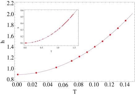
Figure 3: External field as a function of temperature for a given value of the magnetization. Dotted curve in the main figure corresponds to $\langle\phi\rangle=0.9$ while the inset corresponds to $\langle\phi\rangle=0.1$. The continuous lines are fits to quadratic functionalities.

In the upper(lower) region magnetization is greater(lower) than certain value $\langle\phi\rangle>\phi_{0}$ ($\langle\phi\rangle<\phi_{0}$) with $\phi_{0}=0.9$ for the main figure and $\phi_{0}=0.1$ for the inset. The monotony and functionality of curves in figure 3 is independent of the specific value of $\phi_{0}$ even in the vicinity of $\phi_{0}=1$ that represents the limit of the modulated structures. In other words, if we define as ferromagnetic a more real not-completely-saturated state where $\langle\phi\rangle>1-\epsilon$, then figure 3 would be in disagreement with theoretical results for other thin film models.Garel and Doniach (1982) Since $\epsilon$ can be a sufficiently small value, the last definition is pretty near to what can be observed experimentally.

This phenomenology is in good agreement not only with experimental worksSaratz et al. (2010b) but also with some analytical approaches of ultrathin magnetic films considering only striped and uniform phases.Abanov et al. (1995) However, as can be seen from the figure, we obtain a quadratic fit for the temperature functionality that is valid for all values of $\phi_{0}$, instead of the more complex scaling functionality experimentally observedSaratz et al. (2010a) that is dependent on the critical temperature.

So far, it is not easy to understand where this phenomenology encountered in the frustrated spherical model begins to be disturbed from the fact that this model does not recover the phase transition, even in the pure ferromagnetic case in $d=2$. Nevertheless, there is an acceptable agreement with the standard features established in literature for frustrated systems and, moreover, the fact that the local field is bounded in some way seems to have good implications in modeling the behavior of the system in the presence of an external field at $T>0$. This suggests the necessity of finding a near model in which the fundamental limitations already mentioned could be overcome.

IV.1 Extension of the model

Any modification of the standard spherical model must be done in a way that improves the basic characteristics involved in the probable establishment of the ordered phase. Lets consider again the spherical restriction (2) but now writing it in the local way

$$\int_{V_{\vec{n}}}\phi^{2}(\vec{x})d^{d}x=m^{2}V$$ (44)

where $\vec{n}$ is a discrete $d$-dimensional counter vector and $V_{\vec{n}}$ represents certain $d$-dimensional volumes of finite constant size. These finite volumes do not overlaps each other and completely fill the spatial region $\Omega$, so the limit $\Omega\rightarrow\infty$ implies an infinite number of such finite regions. It is over these finite volumes that the spherical constrain is now performed. This is a closer approximation to what actually happens in many real system.

Following the same Langevin formalism as in section (II) but now including the multiple restrictions (44) we reach to the dynamical equation

$$\frac{\partial\phi(\vec{x},t)}{\partial t} = \nabla^{2}\phi(\vec{x})-\frac{1}{\delta}\int_{\Omega}d^{d}x^{\prime}J(\vec{x}-\vec{x}^{\prime})\phi(\vec{x}^{\prime})$$ (45)

$$+ h-\lambda_{\vec{n}}(t)\phi(\vec{x})+\eta(\vec{x},t)$$

that is virtually similar to that of (4) with the exception that $\lambda$ is now also dependent on the space region through the counter $\vec{n}$. It means that there is an infinite set of Lagrange multipliers each one corresponding to a single finite region $V_{\vec{n}}$.

It is completely plausible to expect that the particular geometry of these finite volumes do not implies substantial difference in the phenomenology of the model. So we may take them as $d$-dimensional cubes with a linear size $2a$. In this assumption it is possible to write the equation of motion in the inverse space as

$$\frac{\partial\phi(\vec{k},t)}{\partial t} = -\left[k^{2}+\frac{1}{\delta}J(k)\right]\phi(\vec{k},t)+h(\vec{k})+\eta(\vec{k},t)$$ (46)

$$+ \sum_{\vec{n}}\lambda_{\vec{n}}(t)\int\frac{d^{d}k^{\prime}}{(2\pi)^{d}}\phi(\vec{k}^{\prime},t)\hat{Q}_{\vec{n}}(\vec{k}-\vec{k}^{\prime})$$

where

$$\hat{Q}_{\vec{n}}(\vec{k}-\vec{k}^{\prime}) = \int_{V_{\vec{n}}}e^{i(\vec{k}-\vec{k}^{\prime})\cdot\vec{x}}d^{d}x$$ (47)

$$= \left[\prod_{\alpha=1}^{d}\frac{2\sin[(k^{\prime}_{\alpha}-k_{\alpha})a]}{k^{\prime}_{\alpha}-k_{\alpha}}\right]e^{i(\vec{k}^{\prime}-\vec{k})\cdot\vec{r}}$$

and $\vec{r}=(2\vec{n}+\vec{1})a$.

The more complex but yet linear model thus modified is a very good candidate for observing the transition to the ordered phase in lower dimensions. The modification is substantial with respect to the standard spherical model in which temperature can always destroy the saturated phase, driving the system to multiple non-homogeneous configurations and yet holding the spherical constraint. In this new approach infinite constraints guaranties that, below certain temperature, once the correlation length becomes greater than the typical size $a$ of the spherically constrained volumes, these volumes behaves as fully-magnetized entities not allowing internal inhomogeneities. This fact may eventually drive the system to the Ising universality class or, at least, to a new interesting phenomenology in which the statistical behavior must have a change around some temperature value dependent on the physically meaningful parameter $a$.

It is worth to note that equation (46) admits the trivial paramagnetic solution as the limit case in which all Lagrange multipliers are identical $\lambda_{\vec{r}}=\lambda$. As can be demonstrated

$$\sum_{\vec{n}}\hat{Q}_{\vec{n}}(\vec{k}-\vec{k}^{\prime})=(2\pi)^{d}\delta(\vec{k}-\vec{k}^{\prime})$$ (48)

and then equation (46) becomes the already solved equation (10). This limit is thus associated in the modified model with the high temperatures region. In this conditions the correlation length is so small that the spherical restriction over the complete system has the same effect that if it were done over the finite volumes.

V Conclusions

The Langevin dynamics of the spherical model has been solved in the long times limit considering isotropic competing interactions. The general asymptotic functionality of spatial and self-correlations is found to be equivalent to that of Ginzburg-Landau model in the Hartree self-consistent field approximation.Díaz-Méndez et al. (2010) The work was done studying the ensemble of disordered realizations, and we do not verify any standard glassy transition as that predicted for near models.Tarzia and Coniglio (2006) Nevertheless, for low temperatures the system evolves to a mosaic of randomly oriented modulated structures, very similar to that of the glass state. And moreover, if temperature is sufficiently small, this configuration develops an extended aging dynamics up to times far beyond any laboratory scale.

We also found that, for any fixed magnetization, the $h$-$T$ curve has a quadratic, growing functionality. In particular, very near the saturation, where the real system must pass from the modulated to the ferromagnetic state, the monotony of this functionality is a very important issue. It suggests a possible interpretation based on the spin-bound for recently experimental observations on the phase diagram of ultrathin magnetic films.Saratz et al. (2010a) Anyway, the fundamental impossibility of the classical spherical model to see the phase transition is also the responsible of the non-saturation of the system at any finite temperature. In this sense, a model carrying the nice properties arising from the spherical restriction, but capable, as the Ginzburg-Landau, to account for the phase transition,Mendoza-Coto et al. (2010) would be an important step forward.

Such a model is introduced by means of the substitution of the global restriction by an infinite set of restrictions over finite size regions. The new dynamical equation is derived, and it is shown that this more complex but still linear equation contains the classical spherical model as the limit case of paramagnetic high temperature state. It is suggested that, since the restriction is now over finite volumes in the modified model, once the correlation length becomes greater than this typical volumes size the system must fall into the Ising universality class.

Appendix A Geometrical approach to some spatial correlations.

Firstly we are intended to demonstrate, by means of geometric considerations, that spatial correlation C(R) in an ensemble of perfect striped configurations has an algebraic decaying term of the form $1/R^{(d-1)/2}$, identical to that of expression (39). One can perform such calculation by simply compute the spatial average

$$C(R)=\langle\phi(\vec{x})\phi(\vec{x}+\vec{R})\rangle$$ (49)

with the order parameter taken as

$$\phi(\vec{x})=\phi_{0}\ \mathrm{cos}(\vec{k}_{0}\cdot\vec{x}+\Phi)$$ (50)

where $\Phi\in[0,2\pi]$ is included to represent the arbitrary relative position between the modulated structure and the axes origin.

$d=1$

In one dimension the modulated structure can be written

$$\phi(x)=\phi_{0}\ \mathrm{cos}(k_{0}x+\Phi)$$ (51)

and the integration is simply over $\Phi$ and $x$. Here, $\Phi$ is the random variable containing all the relative displacements (phase) of the modulated structure with respect to the position $x$. The probability of finding a value between $\Phi$ and $\Phi+d\Phi$ is equal to $d\phi/2\pi$. On the other hand, the spatial average is performed multiplying the spatial integral with limits $\pm L$ by a normalization factor $1/2L$. So, we have to carry out the calculation

$$C(R) = \lim_{L\to\infty}\int_{0}^{2\pi}\frac{d\Phi}{2\pi}\int_{-L}^{L}\frac{dx}{2L}\$$ (52)

$$\times \ \phi_{0}\ \cos(k_{0}x+\Phi+k_{0}R)$$

$$\times \phi_{0}\ \cos(k_{0}x+\Phi)$$

that leads to a perfect sinusoidal result

$$C(R)=\frac{\phi_{0}^{2}}{2}\cos(k_{0}R)$$ (53)

$d=2$

Here we have to consider also the multiple angular orientations of the modulated structures $\vec{k}_{0}$ with respect to the axes origin. Now we have

$$\phi(\vec{x})=\phi_{0}\ \mathrm{cos}(\vec{k}_{0}\cdot\vec{x}+\Phi)$$ (54)

Using polar coordinates we may write $\vec{k}_{0}=(k_{0},\alpha)$ and $\vec{x}=(r,\theta)$. Now the random variables are the phase $\Phi$ and the plane orientation of the structure $\alpha$. In this way, the probability of having a stripes configuration with values around certain $\Phi$ and $\alpha$ is

$$P(\Phi,\alpha)d\Phi\ d\alpha=\frac{d\Phi}{2\pi}\frac{d\alpha}{2\pi}$$ (55)

And we have to integrate also the spatial average in polar coordinates. So, the calculation is

$$C(R) = \lim_{L\to\infty}\int_{0}^{2\pi}\frac{d\Phi}{2\pi}\int_{0}^{2\pi}\frac{d\alpha}{2\pi}\int_{0}^{2\pi}\int_{0}^{L}\frac{r\ dr\ d\theta}{\pi L^{2}}$$ (56)

$$\times \ \phi_{0}\ \cos(\vec{k}_{0}\cdot\vec{x}+\Phi+\vec{k}_{0}\cdot\vec{R})$$

$$\times \phi_{0}\ \cos(\vec{k}_{0}\cdot\vec{x}+\Phi)$$

leading to

$$C(R)=\frac{\phi_{0}^{2}}{2}\mathrm{J}_{0}(k_{0}R)=\frac{\phi_{0}^{2}}{2}\frac{\cos(k_{0}R-\pi/4)}{(k_{0}R)^{1/2}}$$ (57)

$d=3$

Following the same analysis one starts now from an expression of $\phi$

$$\phi(\vec{x})=\phi_{0}\ \mathrm{cos}(\vec{k}_{0}\cdot\vec{x}+\Phi)$$ (58)

in which $\vec{k}_{0}$ and $\vec{x}$ are three-dimensional vectors thus representing alternating oriented laminae well-known in literature. With a reasoning very close to that of $d=2$, we use spherical coordinates and write vector as $\vec{k}_{0}=(k_{0},\alpha,\psi)$ and $\vec{x}=(r,\theta,\varphi)$. The multiple orientations are given now by $\alpha$ and $\psi$ and the stripes are characterized by fixing $\Phi$, $\alpha$ and $\psi$ in such a way that

$$P(\Phi,\alpha,\psi)d\Phi\ d\alpha\ d\psi=\frac{d\Phi}{2\pi}\frac{d\alpha}{2\pi}\frac{\sin(\psi)d\psi}{2}$$ (59)

and taken the proper normalization for the spatial average in spherical coordinates

$$C(R) = \lim_{L\to\infty}\int_{0}^{2\pi}\frac{d\Phi}{2\pi}\int_{0}^{\pi}\int_{0}^{2\pi}\frac{\sin(\psi)\ d\psi\ d\alpha}{4\ \pi}$$ (60)

$$\times \int_{0}^{\pi}\int_{0}^{2\pi}\int_{0}^{L}\frac{r^{2}\ \sin(\theta)\ dr\ d\theta\ d\varphi}{\frac{4}{3}\pi L^{3}}$$

$$\times \ \phi_{0}\ \cos(\vec{k}_{0}\cdot\vec{x}+\Phi+\vec{k}_{0}\cdot\vec{R})$$

$$\times \phi_{0}\ \cos(\vec{k}_{0}\cdot\vec{x}+\Phi)$$

This leads to

$$C(R)=\frac{\phi_{0}^{2}}{2}\frac{\sin(k_{0}R)}{k_{0}R}=\frac{\phi_{0}^{2}}{2}\frac{\cos(k_{0}R-\pi/2)}{(k_{0}R)}$$ (61)

Finally, from expressions (53), (57) and (61) one can write, in the approximation $k_{0}R\gg 1$, the following form of $C(R)$ as function of the space dimension.

$$C(R)=\frac{\phi_{0}^{2}}{2}\frac{\cos[k_{0}R-(d-1)\frac{\pi}{4}]}{(k_{0}R)^{\frac{d-1}{2}}}$$ (62)

and this is exactly the same functionality appearing in (39) for spatial correlations, obtained in a completely different way.

A.1 Glassy spatial correlation

Lets analyze now the spatial correlation in a configuration of mosaics of randomly oriented modulated structures. In our approach we divide the space in squared $d$-dimensional volumes of equal linear size $L$ inside which the local parameter is in a perfect striped pattern. The orientation of the modulated structures changes randomly from one area to the other. Under this condition one may write

$$\phi(\vec{x})=\phi_{0}\ \mathrm{cos}(\vec{k}_{0}[\vec{x}]\cdot\vec{x}+\Phi[\vec{x}])$$ (63)

where it has been explicitly pointed the dependence of $\vec{k}_{0}$ and $\Phi$ with $\vec{x}$ through squared brackets. This dependence is quite simple: while the modulus $k_{0}$ is constant over all the space, the relative phase $\Phi$ and the rest of the $d-1$ values $\Omega_{i}$ of the orientational components of $\vec{k}_{0}$ are constant only inside the limits of the finite regions and varies randomly between regions. So, we have to compute the average

$$C(R) = \phi_{0}^{2}\ \langle\cos(\vec{k}_{0}[\vec{x}]\cdot\vec{x}+\Phi[\vec{x}])\times$$

$$\times \cos(\vec{k}_{0}[\vec{x}+\vec{R}]\cdot(\vec{x}+\vec{R})+\Phi[\vec{x}+\vec{R}])\rangle$$

that is

$$C(R) \propto \phi_{0}^{2}\ \int d^{d}x\int d^{(d-1)}\Omega\ \cos(\vec{k}_{0}[\vec{x}]\cdot\vec{x}+\Phi[\vec{x}])\times$$ (65)

$$\times \cos(\vec{k}_{0}[\vec{x}+\vec{R}]\cdot(\vec{x}+\vec{R})+\Phi[\vec{x}+\vec{R}])$$

One may note that, for $R>L$, that is, at distances higher that the typical domain size, the above expression becomes zero. This result is consistent with the exponential decay (42) in which the non-zero value of spatial correlations establishes up to certain length. For distances higher than this length the correlation suddenly vanishes.

References

- Gleiser et al. (2003) P. M. Gleiser, F. A. Tamarit, S. A. Canas, and M. Montemurro, Phys. Rev. B 68, 134401 (2003).
- Jagla (2004) E. A. Jagla, Phys. Rev. E 70, 046204 (2004).
- Nicolao and Stariolo (2007) L. Nicolao and D. A. Stariolo, Phys. Rev. B 76, 054453 (2007).
- Díaz-Méndez and Mulet (2010) R. Díaz-Méndez and R. Mulet, Phys. Rev. B 81, 184420 (2010).
- Garel and Doniach (1982) T. Garel and S. Doniach, Phys. Rev. B 26, 325 (1982).
- Roland and Desai (1990) C. Roland and R. C. Desai, Phys. Rev. B 42, 6658 (1990).
- Pighín and Cannas (2003) S. A. Pighín and S. A. Cannas, Phys. Rev. B 68, 134401 (2003).
- Mulet and Stariolo (2007) R. Mulet and D. A. Stariolo, Phys. Rev. B 75, 064108 (2007).
- Rosensweig et al. (1983) R. E. Rosensweig, M. Zahn, and R. Shumovich, J. Magn. Magn. Mater. 39, 127 (1983).
- Seul and Wolfe (1992) M. Seul and R. Wolfe, Phys. Rev. A 46, 7519 (1992).
- Seul and Andelman (1995) M. Seul and D. Andelman, Science 267, 476 (1995).
- Saratz et al. (2010a) N. Saratz, A. Lichtenberger, O. Portmann, U. Ramsperger, A. Vindigni, and D. Pescia, Phys. Rev. Lett. 104, 077203 (2010a).
- Berlin and Kac (1952) T. H. Berlin and M. Kac, Phys. Rev. 86, 821 (1952).
- Baxter (1982) R. J. Baxter, Exactly solved models in statistical mechanics. (Academic Press, London, 1982).
- Brody (1994) D. C. Brody, Phys. Rev. E 49, 3665 (1994).
- Cannas et al. (2000) S. A. Cannas, D. A. Stariolo, and F. A. Tamarit, Physica A 294, 362 (2000).
- Grousson et al. (2000) M. Grousson, G. Tarjus, and P. Viot, Phys. Rev. E 62, 7781 (2000).
- Grousson et al. (2002) M. Grousson, V. Krakoviack, and G. Tarjus, Phys. Rev. E 66, 26126 (2002).
- Prozorov et al. (2008) R. Prozorov, A. F. Fidler, J. Hoberg, and P. C. Canfield, Nature Phys. 4, 327 (2008).
- Tarzia and Coniglio (2006) M. Tarzia and A. Coniglio, Phys. Rev. Lett. 96, 075702 (2006).
- Díaz-Méndez et al. (2010) R. Díaz-Méndez, A. Mendoza-Coto, R. Mulet, L. Nicolao, and D. A. Stariolo, arXiv:1011.5137v1, submitted to Phys. Rev. B (2010).
- Mendoza-Coto et al. (2010) A. Mendoza-Coto, R. Díaz-Méndez, R. Mulet, L. Nicolao, and D. A. Stariolo, to be published (2010).
- Cugliandolo and Dean (1995) L. F. Cugliandolo and D. S. Dean, J. Phys. A: Math. Gen. 28 (1995).
- Tarzia and Coniglio (2007) M. Tarzia and A. Coniglio, Phys. Rev. E 75, 011410 (2007).
- Godrèche and Luck (2000) C. Godrèche and J. M. Luck, J. Phys. A: Math. Gen. 33, 9141 (2000).
- Saratz et al. (2010b) N. Saratz, A. Lichtenberger, O. Portmann, U. Ramsperger, A. Vindigni, and D. Pescia, Phys. Rev. B 82, 184416 (2010b).
- de Gennes (1972) P. G. de Gennes, Solid State Commun. 10, 753 (1972).
- Spivak and Kivelson (2004) B. Spivak and S. A. Kivelson, Phys. Rev. B 70, 155114 (2004).
- Abanov et al. (1995) A. Abanov, V. Kalatsky, V. L. Pokrovsky, and W. M. Saslow, Phys. Rev. B 51, 1023 (1995).