Modeling the Near-Surface Shear Layer: Diffusion Schemes Studied With CSS

Abstract

As we approach solar convection simulations that seek to model the interaction of small-scale granulation and supergranulation and even larger scales of convection within the near-surface shear layer (NSSL), the treatment of the boundary conditions and minimization of sub-grid scale diffusive processes become increasingly crucial. We here assess changes in the dynamics and the energy flux balance of the flows established in rotating spherical shell segments that capture much of the NSSL with the Curved Spherical Segment (CSS) code using two different diffusion schemes. The CSS code is a new massively parallel modeling tool capable of simulating 3-D compressible MHD convection with a realistic solar stratification in rotating spherical shell segments.

1 Introduction

The solar differential rotation profile exhibits prominent radial shear layers near the top and bottom of the convection zone [thomp03, ]. The near-surface shear layer (NSSL) occupies the upper 5% of the Sun by radius, whereas the tachocline begins near the base of the convection zone. The dynamics of the NSSL are governed largely by vigorous granular-scale convection that is driven by radiative cooling and large thermodynamic gradients. The collective interaction of these granular-scale flows (average sizes of 1 Mm, lifetimes of 0.2 hr) is a major component in the formation of supergranular (15-35 Mm, 24 hr) and mesogranular (5-10 Mm, 5 hr) scales [rast03, ; nord09, ].

Given this wide range of spatial and temporal scales, we currently cannot simultaneously model hundreds to thousands of supergranules, solar granulation, and deeper flows. However, we may still be able to characterize the influence of granulation and deep global flows on the NSSL by coupling CSS with global convection models from below [miesch08, ] and with surface convection simulations from above [e.g. rempel09, ; nord09, ]. Such a coupling, whether it is statistical or direct, requires a careful treatment of diffusion and boundary conditions [august10, ]. For instance, low diffusion is necessary to preserve the spatial structure and advective timescales of the downdrafts flowing into the CSS domain from the surface convection above. Given that our grid is five times coarser than that of typical surface convection simulations, this is no easy task.

We have conducted two numerical simulations in a $20^{\circ}$ square patch centered on the equator that encompass most of the NSSL and some of the deep interior, rotating at the solar rate. These simulations explore the effects of turbulent-eddy and slope-limited diffusion schemes with an open lower radial boundary and closed upper boundary; as such they are identical except for the diffusion scheme. The governing equations and numerical approach used in solving them are briefly discussed in §2. The turbulent-eddy and slope-limited diffusion schemes are detailed in §3. The dynamics of the flows established in these simulations are examined in §4.

2 Formulating the Problem

The spherical segment domains used in our simulations involve large portions of the Sun’s inherent spherical geometry, which is necessary to properly capture the effects of rotation on supergranular scales. We use the Curved Shell Segment (CSS) code to model the 3-D dynamics below the solar photosphere. CSS is a modeling tool that solves the compressible Navier-Stokes equations in rotating spherical segments [august10, ]. To simulate the larger scales of motion that are likely to occur in the solar convection zone, a large-eddy simulation (LES) model is employed. The scales that are not explicitly computed in these simulations are parametrized and included in a sub-grid scale model of turbulent transport and diffusion. The governing equations solved in CSS are:

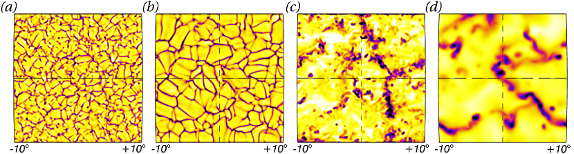
Figure 1: Radial velocities ($u_{r}$) at 0.99 $R_{\odot}$ in (a) the slope-limited diffusion Case 2, and (b) the turbulent-eddy diffusion Case 1, and at 0.95 $R_{\odot}$ in (c) Case 2 and (d) Case 1. Dark tones denote downflows and light tones denote upflows. Scaling values are -1.34 $\mathrm{km\,s^{-1}}$, 0.59 $\mathrm{km\,s^{-1}}$ for (a) and (b) and -0.73 $\mathrm{km\,s^{-1}}$, 0.24 $\mathrm{km\,s^{-1}}$ for (c) and (d), where positive $u_{r}$ points outward.

$$\frac{\partial\rho}{\partial t}+\nabla\cdot\left(\rho\mathbf{u}\right) = 0,$$ (1)

$$\rho\left[\frac{\partial\mathbf{u}}{\partial t}+\left(\mathbf{u}\cdot\nabla\right)\mathbf{u}\right] = -\nabla P-\rho g\hat{\mathbf{r}}+\nabla\cdot\bar{\mathcal{D}}+2\rho\mathbf{u}\times\mathbf{\Omega}+\rho\Omega^{2}\mathbf{R},$$ (2)

$$\rho T\left[\frac{\partial S}{\partial t}+\left(\mathbf{u}\cdot\nabla\right)S\right] = \nabla\cdot\left[\kappa_{S}\mathbf{\nabla}S^{\prime}+\kappa_{0}\frac{\partial\bar{S}}{\partial r}\hat{\mathbf{r}}+\kappa_{r}\mathbf{\nabla}T\right]+\Phi,$$ (3)

$$\bar{\mathcal{D}}_{ij} = \mu\left[\bar{e}_{ij}-\frac{1}{3}\nabla\cdot\mathbf{u}\bar{\delta}_{ij}\right].$$ (4)

The symbols $\rho$, $\mathbf{u}$, $P$, $T$, $S$, $\bar{\mathcal{D}}$, $\bar{e}$, $\bar{\delta}$ are the density, velocity, pressure, temperature, specific entropy, viscous stress tensor, stress tensor, and identity tensor respectively; $\Phi$ is the viscous heating term; the entropy perturbations are $S^{\prime}=S-\langle S\rangle$; the equation of state is $P=\rho^{\gamma}e^{S/C_{V}}$; $\mathbf{\Omega}$ is the angular velocity of the rotating frame; $\mu$ and $\kappa_{S}$ are the turbulent-eddy diffusion of momentum and entropy, and $\kappa_{r}$ is the radiative thermal diffusion; $g$ is the local acceleration due to gravity, where $\mu$, $\kappa_{S}$, $\kappa_{r}$, $\kappa_{0}$, and $g$ are functions of radius only.

The governing equations (Equations 1-3) are evolved on a uniform spatial mesh. Temporal discretization is accomplished using an explicit fourth-order accurate Runge-Kutta time-stepping scheme. The spatial derivatives are computed using a modified sixth-order compact finite difference scheme. A 3-D domain decomposition divides the full spatial mesh into sub-domains. The boundary information necessary to compute spatial derivatives is passed between nearest-neighbor sub-domains using MPI, while computations are shared among the master and slave cores within a supercomputer node using OpenMP.

Currently there are two diffusion schemes implemented in CSS, a turbulent-eddy diffusion (TED) (Equation 3-4) and the slope-limited diffusion (SLD) described in (§3). In the TED scheme, the momentum and entropy diffusivities ($\mu$ and $\kappa_{S}$) are calculated based upon the desired Rayleigh number at the upper boundary with the constraint that the Prandtl number and the dynamic viscosity be constant throughout the domain. There are no directly comparable diffusive parameters in the SLD scheme as the eddy diffusion terms have been dropped. One may still control the level of diffusion, however, with specific choices of which slope-limiter is employed and what characteristic velocity is used at cell interfaces. Figure 1 depicts snapshots of typical flows at two radii from the two diffusion schemes.

3 Slope-Limited Diffusion In CSS

Slope-limited diffusion has many possible formulations, and we have chosen to use a scheme similar to that found in [rempel09, ]. SLD is based upon a piecewise linear reconstruction within a finite volume (cell) centered on each gridpoint of the solution at each time step. The linear reconstruction leads to a solution that has discontinuities at the cell edges. SLD essentially acts to minimize these discontinuities so that the numerical scheme remains stable. While this model of diffusion is not as physically motivated as the eddy diffusion model, it holds many computational advantages. Indeed, with SLD in CSS, a higher level of turbulence is achieved for a given resolution and there is no need to evaluate second-order derivatives, which decreases memory usage by a factor of three and the execution time per time step by a factor of two.

The slope of the linear reconstruction of the solution is given by a ratio of the downwind and upwind cell-center differences ($r_{i}=\Delta_{l}u_{i}/\Delta_{r}u_{i}$). This slope is “limited” by a function $\phi(r_{i})$ that belongs to a class of slope limiters that yield total variation diminishing solutions [leveq02, ]. As in [rempel09, ], we use a linear combination of two such slope limiters, the minmod and superbee limiters. Using the reconstructed slope, values of the primitive variables are computed at the cell edges as $u_{i}^{e}=u_{i}\pm\frac{1}{2}\phi\left(r_{i}\right)\Delta_{r}u_{i}$. The diffusive flux at a cell edge is $f_{i}^{e}=\frac{1}{2}c_{i}^{e}g_{i}^{e}\beta_{i}^{e}\delta u_{i}^{e}$, where $g_{i}^{e}$ is a geometric factor and $c_{i}^{e}$ is a characteristic velocity at a cell edge, and $\delta u_{i}^{e}$ is the difference of the left and right reconstructed values at a cell-edge. To avoid artificial steepening, a local diffusion coefficient $\beta_{i}^{e}$ is constructed such that when $\delta u_{i}^{e}\Delta_{e}u_{i}>0$, $\beta_{i}^{e}=(\delta u_{i}^{e}/\Delta_{e}u_{i})^{2}$ and is zero otherwise. This preserves steep gradients and yields a fourth-order upwind diffusion scheme [rempel09, ].

With the diffusive fluxes at each edge of a given cell as above, the diffusion at the center of a cell is $D_{i}=\left(f_{i}^{r}-f_{i}^{l}\right)/\Delta x_{i}$, where $\Delta x_{i}$ is the grid spacing. This is added to the solution after the full Runge-Kutta time step as $u_{i}=u_{i}+\Delta tD_{i}$. Within our simulations, using the true sound speed in the $c_{i}^{e}$ proves to be overly diffusive. So, for the computation of the $c_{i}^{e}$, the sound speed throughout the computational domain is fixed to a fraction ($\sim 1/10$) of the surface sound speed.

4 Comparing Two Diffusion Schemes

The simulations encompassing a $20^{\circ}\times 20^{\circ}$ domain are relatively low resolution with 128 radial mesh points and 256 points in latitude and longitude. A stellar evolution code is used to establish a realistic initial stratification for the simulations. Since a perfect gas is assumed, the He and H ionization zones cannot currently be simulated. Thus, the impenetrable upper boundary is taken to be 0.995 $R_{\odot}$ in order to exclude most of the radial extent of these zones. The permeable lower boundary is placed at 0.915 $R_{\odot}$, yielding a density contrast across the domain of 400. Each case has the lowest diffusivities that allow numerical stability in the TED (Case 1) and SLD (Case 2) regimes. Using a constant $\nu$ with depth in the TED case is rather restrictive in that the diffusion is larger than necessary away from the upper boundary, but for this preliminary analysis it is sufficient to characterize the differences between the two schemes.

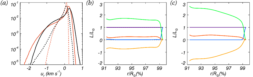
Figure 2: (a) PDFs of radial velocities at 0.99 $R_{\odot}$ (solid line) and 0.95 $R_{\odot}$ (dashed), for Case 2 (black) and Case 1 (red). Time-averaged radial energy flux balances for Case 1 (b) and Case 2 (c), with total flux in purple, radiative flux (blue), enthalpy flux (green), kinetic energy flux (orange), and acoustic flux (red).

Turning to the radial velocity patterns sampled in Figure 1, there is a striking shift toward smaller spatial scales in Case 2 with considerably less power at large scales. At 0.99 $R_{\odot}$ the peak of the spatial power spectrum in Case 1 is around 40 Mm. In Case 2, however, there is a broad peak at scales around 20 Mm, more closely matching the supergranular scales of the Sun. As one descends deeper into the simulations (Figures 1c,d), the flows appear significantly more turbulent in Case 2 than in Case 1.

Indeed, the downflowing structures of Case 2 become much more narrow at depth with many more isolated plumes. The greater turbulence also manifests itself in larger extrema of each of the physical variables. For example, the radial velocities at 0.95 $R_{\odot}$ in Case 2 have extrema that are twice that of Case 1 (Figure 2a). In Case 1, a precipitous drop in the upflowing radial velocity probability density distribution (PDF) outside of about 0.1 $\mathrm{km\,s^{-1}}$ is indicative of just how uniform the upflows are. In stark contrast, the radial velocity PDF of Case 2 has twice the dynamic range, emphasizing that the upflows are indeed much more structured than those of Case 1. While the radial mass flux PDF has higher velocity wings that contribute only one percent to the overall distribution, the bimodal nature of the temperature perturbation PDF has the effect of significantly amplifying the importance of these outlying values. Thus, the net effect of the larger wings in these PDFs is to shift the mean of the enthalpy flux in Case 2 to a higher value. The additional velocity in both the horizontal and radial flows greatly alter the kinetic energy distribution, as in Case 2 where the mean kinetic energy has nearly doubled and correspondingly increased the magnitude of the kinetic energy flux (Figure 2c).

A tentative next step is to have both diffusion schemes active at the same time. This will allow a systematic study on the convergence of solutions as the TED coefficients are lowered to solar values and the SLD takes over as the primary diffusion.

The authors thank Neal Hurlburt and Marc DeRosa for most helpful discussions and their contributions to code development and implementation. This work has been supported by NASA grants NNX08AI57G and NNX10AM74H. The computations were carried out on Pleiades at NASA Ames with SMD grant g26133.

References

- [1] Thompson M J, Christensen-Dalsgaard J, Miesch M S and Toomre J 2003 ARAA 41 599–643
- [2] Rast M P 2003 ApJ 597 1200–1210
- [3] Asplund M, Nordlund A and Stein R F 2009 Living Rev. Solar Phys. 6
- [4] Miesch M S, Brun A S, De Rosa M L and Toomre J 2008 ApJ 673 557–575
- [5] Rempel M, Schüssler M and Knölker M 2009 ApJ 691 640–649
- [6] Hurlburt N E, DeRosa M L, Augustson K C and Toomre J 2010 (ASP Conf. Ser. vol 440)
- [7] LeVeque R J 2002 Finite Volume Methods for Hyperbolic Problems (Cambridge Univ. Press)