Gluon condensates in a cold quark gluon plasma

Abstract

The quark gluon plasma which has been observed at RHIC is a strongly interacting system and has been called sQGP. This is a system at high temperatures and almost zero baryon chemical potential. A similar system with high chemical potential and almost zero temperature may exist in the core of compact stars. Most likely it is also a strongly interacting system. The strong interactions may be partly due to non-perturbative effects, which survive after the deconfinement transition and which can be related with the non-vanishing gluon condensates in the sQGP. In this work, starting from the QCD Lagrangian we perform a gluon field decomposition in low (“soft”) and high (“hard”) momentum components, we make a mean field approximation for the hard gluons and take the matrix elements of the soft gluon fields in the plasma. The latter are related to the condensates of dimension two and four. With these approximations we derive an analytical expression for the equation of state, which is compared to the MIT bag model one. The effect of the condensates is to soften the equation of state whereas the hard gluons significantly increase the energy density and the pressure.

I Introduction

One of the most interesting results of the RHIC program is the discovery of an extremely hot and dense state of matter made of quarks and gluons in a deconfined phase and which behaves like an ideal fluid shu . While the production of such a plasma of quarks and gluons had been predicted, it was a surprise to find that this system is strongly interacting and very different from the originally expected gas of almost non-interacting quarks and gluons, described by perturbative QCD. This state has been called strongly interacting quark gluon plasma (sQGP) and there are many approaches to study its properties. The most fundamental approach is provided by lattice QCD latt . Since lattice QCD has still some limitations, such as the difficulty in dealing with systems with large baryon chemical potential, there are several models (see, for example, gelman ; gardim09 ; bannur08 ) which incorporate the essential features of the full theory and which can be employed to study the sQGP. In some of them gelman ; gardim09 the sQGP is treated as a gas of quasi-particles, in which the quarks and gluons have an effective mass. In some works, such as in gelman ; litim , the sQGP was treated with semi-classical methods. In gelman the color charges were assumed to be large and classical obeying Wong equations of motion. In this approach the quantum effects in the QGP are basically reduced to generate thermal-like masses and cause the effective coupling to run to larger values at smaller values of the temperature.

The medium created in heavy ion collisions has high temperature and zero baryon chemical potential. On the other corner of the phase space, we find the QGP at zero temperature and high baryon number. Presumably, this kind of system exists in the core of dense stars. This cold QGP has a richer phase structure and at high enough chemical potential we may have a color superconducting phase. Because of the limitations of lattice calculations in this domain and also because of the lack of experimental information, the cold QGP is less known than the hot QGP. Nevertheless it is quite possible that it shares some features with the hot plasma, being also a strongly interacting and semi-classical system.

In this work we shall study the non-perturbative effects in the cold QGP generated by the residual dimension two and dimension four condensates, using a mean field approximation.

In the vacuum, non-perturbative effects have been successfully understood in terms of the QCD condensates, i.e., vacuum expectation values of quark and gluon “soft” (low momentum) fields. The best known are the dimension three quark condensate and the dimension four gluon condensate naricond . These condensates can, in principle, be computed in lattice QCD or with the help of models. In practice, since they are vacuum properties and therefore universal, they can be extracted from phenomenological analyses of hadron masses, as it is customary done in QCD sum rules nnl . The condensates are expected to vanish in the limit of very high temperature or chemical potential. However, it has been suggested that they may survive after the deconfinement transition both in the high temperature miller07 ; rede and in the high chemical potential cases zhit05 . For our purposes the relevant gluon condensates are those of dimension four naricond , $\big{\langle}0\big{|}\frac{\alpha_{s}}{\pi}{F}^{2}\big{|}0\big{\rangle}$ ($=\langle F^{2}\rangle$), and of dimension two dudal , $\big{\langle}0\big{|}g^{2}{A}^{2}\big{|}0\big{\rangle}$ ($=\langle g^{2}A^{2}\rangle$).

We shall derive an equation of state (EOS) for the cold QGP, which may be useful for calculations of stellar structure. Our EOS can be considered an improved version of the EOS of the MIT bag model, which contains both the non-perturbative effects coming from the residual gluon condensates and the perturbative effects coming from the hard gluons, which are enhanced by the high quark density. As it will be seen, the effect of the condensates is to soften the EOS whereas the hard gluons significantly increase the energy density and the pressure.

II The equation of state

In this section we develop a mean field approximation for QCD, extending previous works along the same line shakin ; shakinn ; tezuka ; lovas ; fukuda . The Lagrangian density of QCD is given by:

$${\mathcal{L}}_{QCD}=-{\frac{1}{4}}F^{a}_{\mu\nu}F^{a\mu\nu}+\sum_{q=1}^{N_{f}}\bar{\psi}^{q}_{i}\Big{[}i\gamma^{\mu}(\delta_{ij}\partial_{\mu}-igT^{a}_{ij}G_{\mu}^{a})-\delta_{ij}m_{q}\Big{]}\psi^{q}_{j}$$ (1)

where

$$F^{a\mu\nu}=\partial^{\mu}G^{a\nu}-\partial^{\nu}G^{a\mu}+gf^{abc}G^{b\mu}G^{c\nu}$$ (2)

The summation on $q$ runs over all quark flavors, $m_{q}$ is the mass of the quark of flavor $q$, $i$ and $j$ are the color indices of the quarks, $T^{a}$ are the SU(3) generators and $f^{abc}$ are the SU(3) antisymmetric structure constants. For simplicity we will consider only light quarks with the same mass $m$. Moreover, we will drop the summation and consider only one flavor. At the end of our calculation the number of flavors will be recovered. Following shakin ; shakinn , we shall start writting the gluon field as:

$$G^{a\mu}={A}^{a\mu}+{\alpha}^{a\mu}$$ (3)

where ${A}^{a\mu}$ and ${\alpha}^{a\mu}$ are the low (“soft”) and high (“hard”) momentum components of the gluon field respectively. The former will be responsible for the long range and low momentum transfer, non-perturbative processes whereas the latter will be relevant in the short distance perturbative processes. The field decomposition made above requires the choice of an energy scale defining the frontier between soft and hard. This energy scale, $E$, lies in the range $\Lambda_{QCD}<E<1\,\,\mbox{GeV}$. In principle, the dependence of the results on this choice can be studied with the renormalization group techniques. Accurate results would also require the knowledge of the scale dependence of the in-medium gluon condensates, which in our case is poor. Therefore, in order to keep the simplicity of our approach, we will not specify the separation scale and will assume that ${A}^{a\mu}$ represents the soft modes which populate the vacuum and ${\alpha}^{a\mu}$ represents the modes for which the running coupling constant is small.

Inserting (3) into (2) we obtain:

$$F^{a\mu\nu}=(\partial^{\mu}A^{a\nu}-\partial^{\nu}A^{a\mu}+gf^{abc}A^{b\mu}A^{c\nu})+(\partial^{\mu}{\alpha}^{a\nu}-\partial^{\nu}{\alpha}^{a\mu}+gf^{abc}{\alpha}^{b\mu}{\alpha}^{c\nu})$$

$$+gf^{abc}{A}^{b\mu}{\alpha}^{c\nu}+gf^{abc}{\alpha}^{b\mu}{A}^{c\nu}$$ (4)

In the above expression the coupling is running and is large (small) when attached to ${A}^{a\mu}$ (${\alpha}^{a\mu}$). The mixed terms, such as $gf^{abc}{\alpha}^{b\mu}{A}^{c\nu}$, are assumed to be dominated by the large couplings.

II.1 The mean field approximation

In a cold quark gluon plasma the density is much larger than the ordinary nuclear matter density. These high densities imply a very large number of sources of the gluon field. With intense sources the bosonic fields tend to have large occupation numbers at all energy levels, and therefore they can be treated as classical fields. This is the famous approximation for bosonic fields used in relativistic mean field models of nuclear matter serot . It has been applied to QCD in the past tezuka and amounts to assume that the “hard” gluon field, ${\alpha}_{\mu}^{a}$, is simply a function of the coordinates serot :

$${\alpha}_{\mu}^{a}={\alpha}_{0}^{a}\,\delta_{\mu 0}$$ (5)

In fact, for cold nuclear matter, it is further assumed that ${\alpha}_{\mu}^{a}$ is constant in space and time serot :

$$\partial_{\nu}{\alpha}^{a}_{\mu}=0$$ (6)

As a consequence of this approximation, the term $gf^{abc}{\alpha}_{0}^{b}{\alpha}_{0}^{c}$ will vanishe because of the color symmetry. We also assume that the soft gluon field ${A}^{a\mu}$ is independent of position and time and thus:

$$\partial^{\nu}{A}^{a\mu}=0$$ (7)

Substituting (5), (6) and (7) into (4) we have $F^{a\mu\nu}=gf^{abc}(A^{b\mu}A^{c\nu}+{A}^{b\mu}{\alpha}_{0}^{c}\delta^{\nu 0}+{\alpha}_{0}^{b}\delta^{\mu 0}{A}^{c\nu})$. Inserting this into (1), the QCD Lagrangian simplifies to:

$${\mathcal{L}}_{QCD}=-{\frac{g^{2}\,f^{abc}f^{ade}}{4}}\Big{[}{A}^{b}_{\mu}{A}^{c}_{\nu}{A}^{d\mu}{A}^{e\nu}$$

$$+{A}^{b}_{\mu}{A}^{c}_{\nu}{A}^{d\mu}{\alpha}_{0}^{e}\delta^{0\nu}+{A}^{b}_{\mu}{A}^{c}_{\nu}{\alpha}_{0}^{d}\delta^{0\mu}{A}^{e\nu}+{A}^{b}_{\mu}{\alpha}_{0}^{c}\delta_{0\nu}{A}^{d\mu}{A}^{e\nu}+{\alpha}_{0}^{b}\delta_{0\mu}{A}^{c}_{\nu}{A}^{d\mu}{A}^{e\nu}$$

$$+{A}^{b}_{\mu}{\alpha}_{0}^{c}\delta_{0\nu}{\alpha}_{0}^{d}\delta^{0\mu}{A}^{e\nu}+{A}^{b}_{\mu}{\alpha}_{0}^{c}\delta_{0\nu}{A}^{d\mu}{\alpha}_{0}^{e}\delta^{0\nu}+{\alpha}_{0}^{b}\delta_{0\mu}{A}^{c}_{\nu}{A}^{d\mu}{\alpha}_{0}^{e}\delta^{0\nu}+{\alpha}_{0}^{b}\delta_{0\mu}{A}^{c}_{\nu}\,{\alpha}_{0}^{d}\delta^{0\mu}{A}^{e\nu}\Big{]}$$

$$+\bar{\psi}^{q}_{i}\Big{\{}i\gamma^{\mu}[\delta_{ij}\partial_{\mu}-igT^{a}_{ij}({A}_{\mu}^{a}+{\alpha}_{0}^{a}\delta_{0\mu})]-\delta_{ij}m\Big{\}}\psi^{q}_{j}$$ (8)

We shall now replace the soft gluon field ${A}^{b}_{\mu}$ and its powers by the corresponding expectation values in the cold QGP. The product of four fields in the first line of the above equation can be related to the gluon condensate through the relations shakin ; shakinn :

$$\langle{A}^{a}_{\mu}{A}^{b}_{\nu}{A}^{c\rho}{A}^{d\eta}\rangle={\frac{{\phi_{0}}^{4}}{(32)(34)}}\Big{[}g_{\mu\nu}g^{\rho\eta}\delta^{ab}\delta^{cd}+{g_{\mu}}^{\rho}{g_{\nu}}^{\eta}\delta^{ac}\delta^{bd}+{g_{\mu}}^{\eta}{g_{\nu}}^{\rho}\delta^{ad}\delta^{bc}\Big{]}$$ (9)

and

$$-\frac{1}{4}\langle{F}^{a\mu\nu}{F}_{a\mu\nu}\rangle=-\frac{\pi^{2}}{g^{2}}\langle\frac{\alpha_{s}}{\pi}F^{a\mu\nu}F^{a}_{\mu\nu}\rangle=-b\phi_{0}^{4}$$ (10)

where the constant $b$ is given by:

$$b\equiv{\frac{9}{4(34)}}g^{2}$$ (11)

In the second and fourth lines of (8) we have odd powers of ${A}^{a\mu}$ which have vanishing expectation values:

$$\langle{A}^{a\mu}{A}^{b\nu}{A}^{c\rho}\rangle=0$$ (12)

$$\langle{A}^{a\mu}\rangle=0$$ (13)

In the third line of (8) we have the hard gluon mass terms. The expectation value of two soft fields reads: shakin ; shakinn :

$$\langle{A}^{a\mu}{A}^{b\nu}\rangle=-{\frac{\delta^{ab}g^{\mu\nu}}{32}}{\mu_{0}}^{2}$$ (14)

The $\langle g^{2}A^{2}\rangle$ gluon condensate alone is not gauge invariant. While this might be a problem in other contexts, here it is not because it appears always multiplied by other powers of gluon fields, forming gauge invariant objects. The $\langle g^{2}A^{2}\rangle$ condensate is associated shakin ; shakinn with a dynamical gluon mass:

$${m_{G}}^{2}\equiv\bigg{(}{\frac{9}{2}}\bigg{)}\bigg{(}{\frac{1}{16}}\bigg{)}g^{2}{\mu_{0}}^{2}$$ (15)

In spite of the recent progress in the field, still very little is known about $\langle A^{2}\rangle$ at finite (and high) density. In our approach, as in vers , we have $\langle g^{2}A^{2}\rangle$ $<0$ in (14) so ${m_{G}}^{2}$ is positive.

Using expressions (9), (12), (13), (14) and (15) in (8) we arrive at the following effective Lagrangian:

$${\mathcal{L}}=-b{\phi_{0}}^{4}+{\frac{{m_{G}}^{2}}{2}}{\alpha}_{0}^{a}{\alpha}_{0}^{a}+\bar{\psi}^{q}_{i}\Big{(}i\delta_{ij}\gamma^{\mu}\partial_{\mu}+g\gamma^{0}T^{a}_{ij}{\alpha}_{0}^{a}-\delta_{ij}m\Big{)}\psi^{q}_{j}$$ (16)

II.2 Pressure and energy density

From the Lagrangian (16) we can derive the equations of motion:

$${m_{G}}^{2}{\alpha}_{0}^{a}=-g\rho^{a}$$ (17)

$$\Big{(}i\,\delta_{ij}\,\gamma^{\mu}\partial_{\mu}+g\gamma^{0}T^{a}_{ij}{\alpha}_{0}^{a}-m\Big{)}\psi_{j}=0$$ (18)

where $\rho^{a}$ is the temporal component of the color vector current given by:

$$j^{a\nu}=\bar{\psi}_{i}\gamma^{\nu}T^{a}_{ij}\psi_{j}$$ (19)

From the Lagrangain we can obtain the energy-momentum tensor and the energy density of the system through:

$$\varepsilon=<T_{00}>$$ (20)

In the present case the energy-momentum tensor is given simply by:

$${T^{\mu}}_{\nu}={\frac{\partial\mathcal{L}}{\partial(\partial_{\mu}\psi_{i})}}(\partial_{\nu}\psi_{i})\,-\,{g^{\mu}}_{\nu}\mathcal{L}$$ (21)

and consequently:

$$\varepsilon={\frac{\partial\mathcal{L}}{\partial(\partial_{0}\psi_{i})}}(\partial_{0}\psi_{i})-{g}_{00}\mathcal{L}$$ (22)

which, with the use of (16) gives:

$$\varepsilon=i\bar{\psi_{i}}\gamma^{0}(\partial_{0}\psi_{i})-g_{00}\Big{\{}-b{\phi_{0}}^{4}+{\frac{{m_{G}}^{2}}{2}}{\alpha}_{0}^{a}{\alpha}_{0}^{a}+\bar{\psi}^{q}_{i}\Big{(}i\delta_{ij}\gamma^{\mu}\partial_{\mu}+g\gamma^{0}T^{a}_{ij}{\alpha}_{0}^{a}-\delta_{ij}m\Big{)}\psi^{q}_{j}\Big{\}}$$ (23)

Using (18) in the expression above we find

$$\varepsilon=b{\phi_{0}}^{4}-{\frac{{m_{G}}^{2}}{2}}{\alpha}_{0}^{a}{\alpha}_{0}^{a}+i\bar{\psi_{i}}\gamma^{0}(\partial_{0}\psi_{i})$$ (24)

Multiplying (18) by $\bar{\psi_{i}}$ from the left we find:

$$i\psi^{\dagger}_{i}(\partial_{0}\psi_{i})=\psi^{\dagger}_{i}(-i\vec{\alpha}\cdot\vec{\nabla}+\gamma^{0}m)\psi_{i}-g\rho^{a}{\alpha}_{0}^{a}$$ (25)

From the usual Dirac theory applied to the study of nuclear matter we have serot :

$$\psi^{\dagger}_{i}(-i\vec{\alpha}\cdot\vec{\nabla}+\gamma^{0}m)\psi_{i}=3{\frac{\gamma_{Q}}{2{\pi}^{2}}}\int_{0}^{k_{F}}dk\hskip 2.84544ptk^{2}\sqrt{{\vec{k}}^{2}+m^{2}}$$ (26)

In the last two expressions we have:

$$\vec{\alpha}=\left(\begin{array}[]{cc}0&\vec{\sigma}\\ \vec{\sigma}&0\end{array}\right)\ ,\hskip 34.14322pt\gamma^{0}=\left(\begin{array}[]{cc}1&0\\ 0&-1\end{array}\right)$$

where $\vec{\sigma}$ are the standard $2\times 2$ Pauli matrices, the unit entries in $\gamma^{0}$ are $2\times 2$ unit matrices and $\gamma_{Q}$ is the quark degeneracy factor $\gamma_{Q}=2(\mbox{spin})\times 3(\mbox{flavor})$. The sum over all the color states was already performed and resulted in the pre-factor $3$ in the expression above. $k_{F}$ is the Fermi momentum defined by the quark number density $\rho$:

$$\rho=\langle N|\psi^{\dagger}_{i}\psi_{i}|N\rangle={\frac{3}{V}}\sum_{\vec{k},\lambda}\langle N|N\rangle={\frac{3}{V}}\sum_{\vec{k},\lambda}=3{\frac{\gamma_{Q}}{(2\pi)^{3}}}\int d^{3}k=3{\frac{\gamma_{Q}}{2{\pi}^{2}}}\int_{0}^{k_{F}}dk\hskip 2.84544ptk^{2}$$

which gives:

$$\rho={\frac{\gamma_{Q}}{2{\pi}^{2}}}{{k_{F}}}^{3}$$ (27)

In the above expression $|N\rangle$ denotes a state with N quarks. Inserting (26) into (25) and then (25) into (24) we find:

$$\varepsilon=b{\phi_{0}}^{4}-{\frac{{m_{G}}^{2}}{2}}{\alpha}_{0}^{a}{\alpha}_{0}^{a}-g\rho^{a}{\alpha}_{0}^{a}+3{\frac{\gamma_{Q}}{2{\pi}^{2}}}\int_{0}^{k_{F}}dk\hskip 2.84544ptk^{2}\sqrt{{\vec{k}}^{2}+m^{2}}$$ (28)

Using (17) we can eliminate the field ${\alpha}_{0}^{a}$ in the above expression:

$$\varepsilon=b\,{\phi_{0}}^{4}+\bigg{(}{\frac{g^{2}}{2{m_{G}}^{2}}}\bigg{)}\ \rho^{a}\rho^{a}+\,3\,{\frac{\gamma_{Q}}{2{\pi}^{2}}}\int_{0}^{k_{F}}dk\hskip 2.84544ptk^{2}\sqrt{{\vec{k}}^{2}+m^{2}}$$ (29)

We can relate the color charge density $\rho^{a}$ and the quark number density $\rho$. To do this we shall use the notation of gri and write the quark spinor as $\psi_{i}=\psi c_{i}$, where $c_{i}$ is a color vector. We have:

$$\rho^{a}\rho^{a}=(\bar{\psi}_{i}\gamma^{0}T^{a}_{ij}\psi_{j})(\bar{\psi}_{k}\gamma^{0}T^{a}_{kl}\psi_{l})=({\psi}^{\dagger}_{i}T^{a}_{ij}\psi_{j})({\psi}^{\dagger}_{k}T^{a}_{kl}\psi_{l})=({c}^{\dagger}_{i}T^{a}_{ij}c_{j}){\psi}^{\dagger}\psi({c}^{\dagger}_{k}T^{a}_{kl}c_{l}){\psi}^{\dagger}\psi=3\rho^{2}$$ (30)

where we used the relations $\psi^{\dagger}\psi=\rho$ and $({c}^{\dagger}_{i}T^{a}_{ij}c_{j})({c}^{\dagger}_{k}T^{a}_{kl}c_{l})=3$. Performing the momentum integral we arrive at the final expression for the energy density:

$$\varepsilon=\bigg{(}{\frac{3g^{2}}{2{m_{G}}^{2}}}\bigg{)}\ \rho^{2}+b\phi_{0}^{4}+3{\frac{\gamma_{Q}}{2{\pi}^{2}}}\bigg{\{}{\frac{{k_{F}}^{3}\sqrt{{k_{F}}^{2}+m^{2}}}{4}}+{\frac{m^{2}{k_{F}}\sqrt{{k_{F}}^{2}+m^{2}}}{8}}$$

$$-{\frac{m^{4}}{8}}ln\Big{[}{k_{F}}+\sqrt{{k_{F}}^{2}+m^{2}}\ \Big{]}+{\frac{m^{4}}{16}}ln(m^{2})\bigg{\}}$$ (31)

The pressure is given by

$$p={\frac{1}{3}}<T_{ii}>$$ (32)

Repeating the same steps mentioned before and using:

$$\psi^{\dagger}_{i}(-i\vec{\alpha}\cdot\vec{\nabla})\psi_{i}=3{\frac{\gamma_{Q}}{(2\pi)^{3}}}\int d^{3}k\hskip 2.84544pt\bigg{\{}{\frac{{\vec{k}}^{2}}{\sqrt{{\vec{k}}^{2}+m^{2}}}}\bigg{\}}=3{\frac{\gamma_{Q}}{2\pi^{2}}}\int_{0}^{k_{F}}dk\hskip 2.84544ptk^{2}\bigg{\{}{\frac{{\vec{k}}^{2}}{\sqrt{{\vec{k}}^{2}+m^{2}}}}\bigg{\}}$$ (33)

we arrive at:

$$p={\frac{{m_{G}}^{2}}{2}}{\alpha}_{0}^{a}{\alpha}_{0}^{a}-b{\phi_{0}}^{4}+{\frac{\gamma_{Q}}{2\pi^{2}}}\int_{0}^{k_{F}}dk\hskip 2.84544ptk^{2}\bigg{\{}{\frac{{\vec{k}}^{2}}{\sqrt{{\vec{k}}^{2}+m^{2}}}}\bigg{\}}$$ (34)

Performing the momentum integral, using (17) and the relation for $\rho^{a}$ and the quark number density $\rho$ in (34) we obtain the final expression for the pressure:

$$p=\bigg{(}{\frac{3g^{2}}{2{m_{G}}^{2}}}\bigg{)}\ \rho^{2}-b\phi_{0}^{4}+{\frac{\gamma_{Q}}{2{\pi}^{2}}}\bigg{\{}{\frac{{k_{F}}^{3}\sqrt{{k_{F}}^{2}+m^{2}}}{4}}-{\frac{3m^{2}{k_{F}}\sqrt{{k_{F}}^{2}+m^{2}}}{8}}$$

$$+{\frac{3m^{4}}{8}}ln\Big{[}{k_{F}}+\sqrt{{k_{F}}^{2}+m^{2}}\ \Big{]}-{\frac{3m^{4}}{16}}ln(m^{2})\bigg{\}}$$ (35)

The speed of sound $c_{s}$ is given by:

$${c_{s}}^{2}={\frac{\partial p}{\partial\varepsilon}}$$ (36)

In the expressions above, $g$ is small, since it comes always from the coupling between the hard gluons and the quarks. The large coupling is contained in the constants $b$ and $m_{G}$.

Both (31) and (35) have three terms. The first term, proportional to $\rho^{2}$, comes from the purely hard gluonic term appearing in the Lagrangian and from the hard gluon term appearing in the quark equation of motion. The second term, proportional to $\phi_{0}^{4}$, comes exclusively from the soft gluon terms and it has opposite signs in the energy and in the pressure. This is precisely the behavior of the bag constant term in the MIT bag model which has the same origin. The third term comes from the quarks. In short, we can say the both the energy density and the pressure are the sum of three contributions: the hard gluons, the soft gluons and the quarks.

III Numerical results and discussion

We now compare our results (31), (35) and (36), with the corresponding results obtained with the MIT bag model for a gas of quarks at zero temperature serot ; nos2010 :

$${{\varepsilon}_{0}}=\bigg{(}{\frac{9}{4}}\bigg{)}\pi^{2/3}{\rho_{B}}^{4/3}+\mathcal{B}$$ (37)

and

$${{p}_{0}}={\frac{1}{3}}\bigg{(}{\frac{9}{4}}\bigg{)}\pi^{2/3}{\rho_{B}}^{4/3}-\mathcal{B}$$ (38)

and

$${{c_{0}}^{2}}={\frac{\partial p}{\partial\varepsilon}}={\frac{1}{3}}$$ (39)

We choose $\mathcal{B}=110$ MeV fm^-3, which lies in the range ($50<B<200$ MeV fm^-3) used in calculations of stellar structure baldo ; sama ; burg02 . For the comparison we must rewrite (27), (31) and (35) as functions of the baryon density, which is $\rho_{B}={\frac{1}{3}}\rho$.

If we neglect the gluonic terms and choose the quark mass $m$ to be zero in (31) and (35) we can show that they coincide with (37) and (38) with $\mathcal{B}=0$. In this limit, our model reduces to the MIT bag model.

We next consider the MIT bag model with finite $\mathcal{B}$ and our model with massless quarks and soft gluons but no hard gluons. This comparison is meaningful because with these ingredients both models describe the dynamics of free quarks under the influence of a soft gluon background. In this case we can identify our gluonic term with the gluonic component of the MIT bag model, represented by the bag constant. We then obtain an expression for the bag constant in terms of the gluon condensate:

$$\mathcal{B}_{QCD}=b\phi_{0}^{4}=\langle\frac{1}{4}F^{a\mu\nu}F^{a}_{\mu\nu}\rangle$$ (40)

where in the last equality we have used (10) and (11). The above relation has been found in previous works, such as, for example, miller07 . Fixing $\mathcal{B}$ and choosing a reasonable value of the coupling of the soft gluons, $g$, appearing in (10) we can infer the value of the dimension four condensate, $<F^{2}>$, in the deconfined phase. For $\mathcal{B}=110$ MeV fm^-3 and $g=2.7$ (which would correspond to $\alpha_{s}=g^{2}/4\pi=0.6$) we find:

$$\langle{F}^{2}\rangle\,=\,\langle\frac{\alpha_{s}}{\pi}F^{a\mu\nu}F^{a}_{\mu\nu}\rangle\,=\,0.0006\,\,\mbox{GeV}^{4}$$ (41)

In the lack of knowledge of the in-medium dimension two condensate, we use the factorization hypothesis, which, in the notation of Refs. shakin and shakinn , implies the choice $\mu_{0}=\phi_{0}$. As a consequence, (9), (10), (14) and (15) are related and we obtain:

$$\langle g^{2}A^{2}\rangle\,=\,-\sqrt{\frac{(4)(34)\pi^{2}}{9}\langle F^{2}\rangle}\,=\,-0.3\,\,\mbox{GeV}^{2}$$ (42)

which corresponds to a dynamical mass of $m_{G}=290$ GeV. This number is consistent with the values quoted in recent works natale ; aguilar ; sorella , which lie in the range $200<m_{G}<600$ MeV. Finally, the numerical evaluation of (31), (35) and (36) requires the choice of $g$, the coupling of the hard gluons, and of the quark mass, $m$. We choose them to be $g=0.35$ (corresponding to $\alpha_{s}=g^{2}/4\pi=0.01$) and $m=0.02$ GeV.

In Fig. 1 we show the energy density, pressure and speed of sound obtained with (31), (35) and (36) divided by the corresponding MIT values: $\varepsilon_{0}$, $p_{0}$ and $c_{0}$. We observe that, for this set of parameters, our EOS is harder than the MIT one. This can also be seen in the plot of the pressure as a function of the energy density, shown in Fig. 2. In the same range of baryon densities, we have more energy, much more pressure and consequently a larger speed of sound. This behavior can be attributed to the first term of the equations (31) and (35), which comes from the hard gluons. This term is exactly the same both in (31) and (35) and in the limit of high densities becomes dominant yielding $p\simeq\varepsilon$ and hence $c_{s}\rightarrow 1$. Physically, this term represents the perturbative corrections to the MIT approach. Since the quark density is extremely large, even in the weak coupling regime (typical of the hard gluons) the field $\alpha^{a}_{0}$ is intense. A similar situation occurs in the color glass condensate (CGC). In that context, a proton (or nucleus) boosted to very high energies becomes the source of intense gluon fields generated in the weak coupling regime. Also in that case semi-classical methods were applied to study this gluonic system.

In Fig. 3 we plot the energy density (31) (upper panel) and the pressure (35) (lower panel) as a function of the baryon density $\rho_{B}$. We take $\rho_{B}$ always starting at $1.5$ fm^-3. We can observe that the quarks and hard gluons give the dominant contributions both to the energy and to the pressure. Looking at the pressure we see that the hard gluons give a repulsive contribution whereas the soft gluon contribution is attractive. It is interesting to see that our curves follow very closely those of Refs. sama and burg02 , computed with slightly different versions of the MIT bag model.

In Fig. 4 we show the EOS for different choices of the condensates, which are now treated as independent from each other. In the upper panel we fix $\langle F^{2}\rangle$ and vary $\langle g^{2}A^{2}\rangle$, starting from the central value $-0.3$ GeV² and increasing its magnitude. In the lower panel we perform the complementar study keeping $\langle g^{2}A^{2}\rangle$ and increasing the magnitude of $\langle F^{2}\rangle$. As it can be seen, increasing the condensates reduces the pressure and, in the case of $\langle g^{2}A^{2}\rangle$, softens the equation of state. This behavior could be anticipated from Eqs. (31), (35) and from equation of motion (17). Indeed, keeping fixed the coupling and the quark density, when we increase the gluon mass, the field becomes weaker. In a more accurate treatment, with the inclusion of spatial inhomogeneities, the equation of motion (17) would contain a Laplacian term and its solution would show a Yukawa behavior, with the mass $m_{G}$ controlling the screening of the field $\alpha^{a}_{0}$.

In Fig. 5 we show the energy per particle as a function of the baryon density for different values of the gluon condensates. As in the previous figure, in the upper panel we fix $\langle F^{2}\rangle$ and vary $\langle g^{2}A^{2}\rangle$. Increasing $\langle g^{2}A^{2}\rangle$ the energy per particle grows slower with baryon density. The system becomes more compressible. In the lower panel we keep $\langle g^{2}A^{2}\rangle$ fixed and increase the magnitude of $\langle F^{2}\rangle$. Increasing $\langle F^{2}\rangle$ leads, as before, to a more compressible system but the total energy is now larger. For the central values of $\langle F^{2}\rangle$ and $\langle g^{2}A^{2}\rangle$ we obtain values of $\varepsilon/\rho_{B}$ which are compatible with those found in Ref. laura10 for equivalent baryon densities. As it can be seen in all curves, the energy per particle is always much larger than the nucleon mass (939 MeV) and hence the system under consideration can decay into nuclear matter.

To summarize, we have derived an equation of state for the cold QGP, which may be useful for calculations of stellar structure. The derivation is simple and based on three assumptions: i) decomposition of the gluon field into soft and hard components; ii) replacement of the soft gluon fields by their expectation values (“in-medium condensates”) and iii) replacement of the hard gluon fields by their mean-field (classical) values. Our EOS can be considered an improved version of the EOS of the MIT bag model, which contains both the non-perturbative effects coming from the residual gluon condensates and the perturbative effects coming from the hard gluons, which are enhanced by the high quark density. It is reassuring to observe that our EOS has the correct limits, where we recover the MIT bag model results. The parameters are the usual ones in QCD calculations: couplings, masses and condensates. The effect of the condensates is to soften the EOS whereas the hard gluons significantly increase the energy density and the pressure.

Figure 1: Energy density, pressure and speed of sound, as functions of the baryon density, divided by the corresponding MIT values: $\varepsilon_{0}$, $p_{0}$ and $c_{0}$.

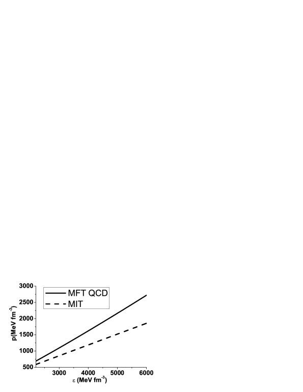
Figure 2: Pressure as a function of the energy density.

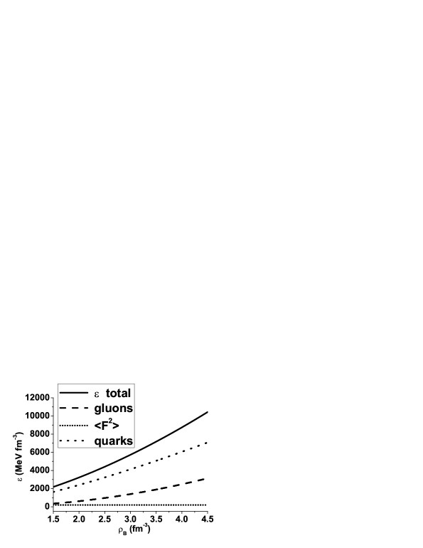
Figure 3: Individual contributions to the energy density and to the pressure: hard gluons , quarks , soft gluons and the sum of the three components.

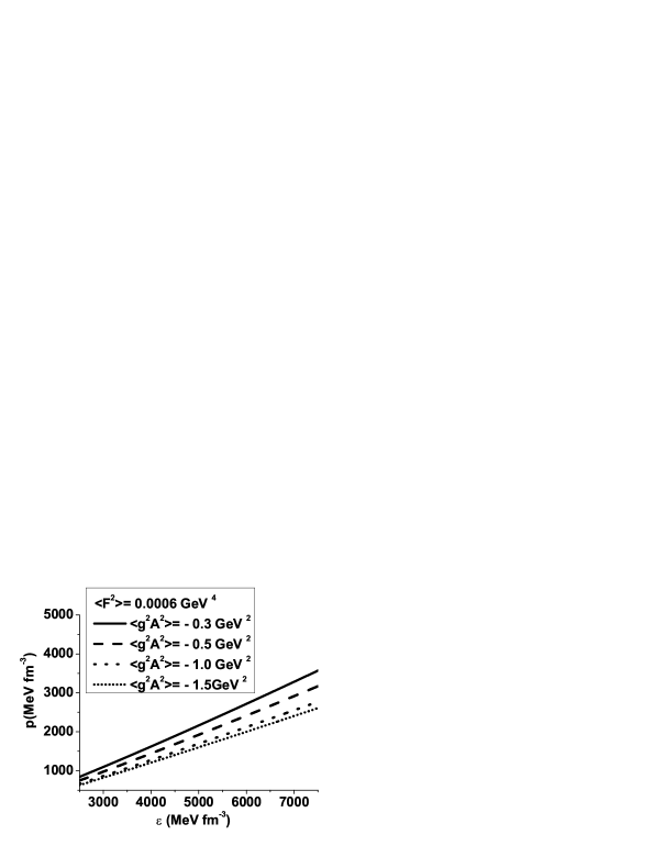
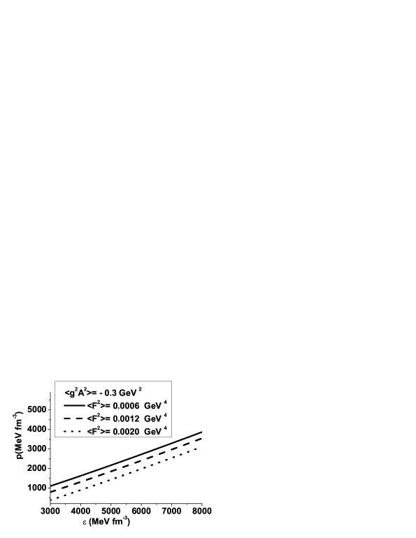
Figure 4: EOS for different values of dimension two and four gluon condensates.

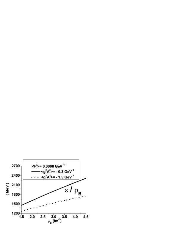
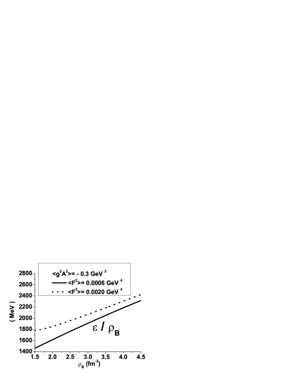
Figure 5: Energy per particle as a function of the baryon density for different values of the gluon condensates.

- (1) E. Shuryak, Prog. Part. Nucl. Phys. 62, 48 (2009).
- (2) A. Bazavov, et al., arXiv:0903.4379 [hep-lat]; Z. Fodor and S.D. Katz, arXiv:0908.3341 [hep-ph]; F. Csikor, et al., JHEP 0405, 046 (2004).
- (3) B.A. Gelman, E.V. Shuryak and I. Zahed, Phys. Rev. C 74, 044908 (2006); ibid. 74, 044909 (2006).
- (4) F. G. Gardim and F. M. Steffens, Nucl. Phys. A 825, 222 (2009); A 797, 50 (2007).
- (5) V.M. Bannur, Phys. Rev. C 78, 045206 (2008).
- (6) D.F. Litim and C. Manuel, Phys. Rev. Lett. 82, 4981 (1999); Nucl. Phys. B 562, 237 (1999); Phys. Rev. D 61, 125004 (2000); Phys. Rep. 364, 451 (2002).
- (7) S. Narison, Phys. Lett. B 693, 559 (2010) and references therein.
- (8) M. Nielsen, F. S. Navarra and S. H. Lee, Phys. Rep. 497, 41 (2010) and references therein.
- (9) D. E. Miller, Phys. Rep. 443, 55 (2007).
- (10) G. Boyd, J. Engles, F. Karsch, E. Laermann, C. Legeland, M. Lutgemeier, and B. Petersson, Nucl. Phys. B 469, 419 (1996).
- (11) M. A. Metlitski and A. R. Zhitnitsky Nucl. Phys. B 731, 309 (2005).
- (12) D. Vercauteren, D. Dudal, J. Gracey, N. Vandersickel and H. Verschelde, Acta Phys. Polon. Supp. 3, 829 (2010); PoS LC2010, 071 (2010); D. Dudal, O. Oliveira and N. Vandersickel, Phys. Rev. D 81, 074505 (2010).
- (13) L. S. Celenza and C. M. Shakin, Phys. Rev. D 34, 1591 (1986).
- (14) X. Li and C. M. Shakin, Phys. Rev. D 71, 074007 (2005).
- (15) H. Tezuka, “Mean Field Approximation to QCD”, INS-Rep.-643 (1987).
- (16) I. Lovas, W. Greiner, P. Hraskǿ and E. Lovas, Phys. Lett. B 156, 255 (1985).
- (17) R. Fukuda, Prog. Theor. Phys. 67, 648 (1982).
- (18) B.D. Serot and J.D. Walecka, Advances in Nuclear Physics 16, 1 (1986).
- (19) H. Verschelde, K. Knecht, K. Van Acoleyen and M. Vanderkelen, Phys. Lett. B 516, 307 (2001).
- (20) D. Griffiths,“Introduction to Elementary Particles”, Chapter 9, John Wiley & Sons Inc. , 1987.
- (21) D. A. Fogaça, L. G. Ferreira Filho and F. S. Navarra, Phys. Rev. C 81, 055211 (2010).
- (22) M. Baldo, P. Castorina, D. Zappal , Nucl. Phys. A 743, 3 (2004).
- (23) F. Sammarruca, arXiv:1009.1172v1 [nucl-th].
- (24) G. F. Burgio, M. Baldo, P. K. Sahu and H. J. Schulze, Phys. Rev. C 66, 025802 (2002).
- (25) A. A. Natale, Nucl. Phys. Proc. Suppl. 199 (2010) 178.
- (26) A. C. Aguilar and A. A. Natale, JHEP 0408, 057 (2004).
- (27) D. Dudal, S. P. Sorella, N. Vandersickel and H. Verschelde, Phys. Rev. D 77, 071501 (2008); D. Dudal, J. A. Gracey, S. P. Sorella, N. Vandersickel and H. Verschelde, Phys. Rev. D 78, 065047 (2008).
- (28) L. Paulucci, E. J. Ferrer, V. de la Incera and J. E. Horvath, arXiv:1010.3041 [astro-ph].