Orthogonal polynomials and expansions for a family of weight functions in two variables

Abstract.

Orthogonal polynomials for a family of weight functions on $[-1,1]^{2}$,

$${\mathcal{W}}_{{\alpha},{\beta},{\gamma}}(x,y)=|x+y|^{2{\alpha}+1}|x-y|^{2{\beta}+1}(1-x^{2})^{\gamma}(1-y^{2})^{{\gamma}},$$

are studied and shown to be related to the Koornwinder polynomials defined on the region bounded by two lines and a parabola. In the case of ${\gamma}=\pm 1/2$, an explicit basis of orthogonal polynomials is given in terms of Jacobi polynomials and a closed formula for the reproducing kernel is obtained. The latter is used to study the convergence of orthogonal expansions for these weight functions.

1. Introduction

Orthogonal polynomials of two variables with respect to a nonnegative weight function that has all moments finite are known to exist ([4]). A basis of orthogonal polynomials can be written down, say, in terms of moments, but such a basis is often hard to work with. For studying orthogonal polynomials and orthogonal expansions, additional structures are often called for. In the case of classical weight functions in two variables, for example, an orthogonal basis can be expressed in terms of classical orthogonal polynomials of one variable. There are, however, not many such examples; each additional one is valuable in its own right.

The purpose of the present paper is to study orthogonal polynomials and orthogonal expansions with respect to a family of weight functions defined on $[-1,1]^{2}$, which includes as a special case

(1.1) $${\mathcal{W}}_{{\alpha},{\beta},{\gamma}}(x,y):=|x-y|^{2{\alpha}+1}|x+y|^{2{\beta}+1}(1-x^{2})^{\gamma}(1-y^{2})^{{\gamma}},$$

where ${\alpha},{\beta},{\gamma}>-1$ and ${\alpha}+{\gamma}+3/2>0$ and ${\beta}+{\gamma}+3/2>0$. In the case ${\alpha}={\beta}=-1/2$, ${\mathcal{W}}_{{\alpha},{\beta},{\gamma}}$ is the product Gegenbauer weight functions, for which an orthogonal basis is given by product Gagenbauer polynomials. We shall show that orthogonal polynomials for this family of weight functions can be expressed in terms of orthogonal polynomials in one variable when ${\gamma}=\pm\frac{1}{2}$. Our study starts from a realization that it is possible to express the orthogonal polynomials with respect to ${\mathcal{W}}_{{\alpha},{\beta},{\gamma}}$ in terms of the Koornwinder polynomials that are orthogonal with respect to the weight function

(1.2) $$W_{{\alpha},{\beta},{\gamma}}(u,v):=(1-u+v)^{\alpha}(1+u+v)^{\beta}(u^{2}-4v)^{{\gamma}}$$

defined on the domain $\Omega$ bounded by two lines and a parabola,

(1.3) $$\Omega:=\{(u,v):1+u+v>0,1-u+v>0,u^{2}>4v\}.$$

Orthogonal polynomials with respect to $W_{{\alpha},{\beta},{\gamma}}$ were first studied by Koornwinder in [7], where an orthogonal basis is uniquely defined and shown to consist of eigenfunctions of two differential operators of order 2 and order 4, respectively. In the case of ${\gamma}=\pm\frac{1}{2}$, the orthogonal polynomials can be given in terms of the Jacobi polynomials of one variable. Further studies were carried out in [9, 13]; in particular, explicit formula for the orthogonal polynomials were derived and various recursive relations were established. The connection to orthogonal polynomials with respect to ${\mathcal{W}}_{{\alpha},{\beta},{\gamma}}$ is somewhat surprising, but simple in retrospect as can be seen by the relation

$${\mathcal{W}}_{{\alpha},{\beta},{\gamma}}(x,y)=4^{-{\gamma}}W_{{\alpha},{\beta},{\gamma}}(2xy,x^{2}+y^{2}-1)|x^{2}-y^{2}|.$$

As a result of the connection, an orthogonal basis for ${\mathcal{W}}_{{\alpha},{\beta},\pm\frac{1}{2}}$ can be given explicitly in terms of the Jacobi polynomials.

An explicit orthogonal basis makes it possible to study orthogonal expansions, for which however it is essential to have access to the reproducing kernel of the space of polynomials of degree at most $n$ in $L^{2}(W)$. It turns out that closed forms of the reproducing kernels for $W_{{\alpha},{\beta},\pm\frac{1}{2}}$ and for ${\mathcal{W}}_{{\alpha},{\beta},\pm\frac{1}{2}}$, respectively, can be given in terms of the reproducing kernels of the Jacobi polynomials. This allows us to prove several results on the convergence of the orthogonal expansions for these weight functions. The results include $L^{p}$ convergence of the partial sum operators and sharp estimate of the Lebesgue constants. It is interesting to note that analogous result on the $L^{p}$ convergence has not been proven for the product Jacobi series on the square (the partial sum is defined in terms of polynomial subspace of total order, see Remark 2.1). In fact, as far as we know, $W_{{\alpha},{\beta},-\frac{1}{2}}$ appears to be the first family of weight functions on the unit square for which a comprehensive study of orthogonal expansions is possible.

The Koornwinder polynomials are derived from the symmetric orthogonal polynomials with respect to the weight function

$$W_{{\alpha},{\beta},{\gamma}}(x+y,xy)|x-y|=(1-x)^{\alpha}(1+x)^{\beta}(1-y)^{\alpha}(1+y)^{\beta}|x-y|^{2\gamma+1},$$

which are the generalized Jacboi polynomials of $BC_{2}$ type. The latter are the first case of the generalized Jacobi polynomials of $BC_{n}$ type studied by several authors (see, e.g. [2, 15]) and they motivated the Jacobi polynomials of Heckman and Opdam [6] associated with root systems. The connection between these $BC_{2}$ polynomials and orthogonal polynomials for ${\mathcal{W}}_{{\alpha},{\beta},{\gamma}}$ appears to be new.

The paper is organized as follows. The following section is a preliminary, where the basic results on orthogonal polynomials are introduced. In Section 3 we recollect properties of orthogonal polynomials for $W_{{\alpha},{\beta},{\gamma}}$ and establish a closed form formula for the reproducing kernel. The orthogonal polynomials for $W_{{\alpha},{\beta},{\gamma}}$ are studied in Section 4. The orthogonal expansions are investigated in Section 5.

2. Preliminary on orthogonal polynomials

In this short section we recall basics on orthogonal polynomials of one variable and two variables, respectively, in two separate subsections.

2.1. Orthogonal polynomials of one variable

Let $w$ be a nonnegative weight function on $[-1,1]$ that has finite moment of all orders. Throughout this paper we denote by $p_{n}$ the orthonormal polynomials of degree $n$ with respect to the weight function $w$, which are uniquely determined by

$$\int_{-1}^{1}p_{n}(x)p_{m}(x)w(x)dx=\delta_{n,m},\quad n,m\geq 0$$

and ${\gamma}_{n}>0$, where ${\gamma}_{n}$ denotes the leading coefficient of the orthogonal polynomial $p_{n}$, that is, $p_{n}(x)={\gamma}_{n}x^{n}+\ldots$. Let $\Pi_{n}$ denote the space of polynomials of degree at most $n$ in one variable. The reproducing kernel of $k_{n}(w;\cdot,\cdot)$ of $\Pi_{n}$ is defined by the relation

$$\int_{-1}^{1}p(y)k_{n}(w;x,y)w(y)dy=p(x),\quad\forall p\in\Pi_{n}.$$

The well known Christoffel-Darboux formula shows that

(2.1) $$k_{n}(w;x,y)=\sum_{k=0}^{n}p_{k}(x)p_{k}(y)=\frac{{\gamma}_{n}}{{\gamma}_{n+1}}\frac{p_{n+1}(x)p_{n}(y)-p_{n+1}(y)p_{n}(x)}{x-y}.$$

The Fourier orthogonal expansion of $f\in L^{2}(w)$ is defined by

$$f=\sum_{n=0}^{\infty}\widehat{f}_{n}p_{n}\quad\hbox{and}\quad\widehat{f}_{n}:=\int_{-1}^{1}f(y)p_{n}(y)w(y)dy,$$

where the equality holds in the $L^{2}(w)$ sense by the standard Hilbert space theory and the fact that polynomials are dense in $L^{2}(w)$. The partial sum operator $s_{n}f$ of this expansion is given by

(2.2) $$s_{n}(w;f,x):=\sum_{k=0}^{n}\widehat{f}_{k}p_{k}=\int_{-1}^{1}f(y)k_{n}(w;x,y)w(y)dy,$$

where the second equal sign follows from the definition of $k_{n}(w;\cdot,\cdot)$.

The Jacobi weight function $w=w_{{\alpha},{\beta}}$ ($w\in J$) is defined by

$$w_{{\alpha},{\beta}}(x):=(1-x)^{\alpha}(1+x)^{\beta},\qquad{\alpha},{\beta}>-1.$$

The Jacobi polynomials are orthogonal with respect to $w_{{\alpha},{\beta}}$ and they are given explicitly as an hypergeometric function

$$P_{n}^{({\alpha},{\beta})}(x,y)=\frac{({\alpha}+1)_{n}}{n!}{}_{2}F_{1}\left(\begin{matrix}-n,n+{\alpha}+{\beta}+1\\ {\alpha}+1\end{matrix};\frac{1-x}{2}\right).$$

These polynomials satisfy the orthogonal conditions

$$c_{{\alpha},{\beta}}\int_{-1}^{1}P_{n}^{({\alpha},{\beta})}(x)P_{m}^{({\alpha},{\beta})}(x)w_{{\alpha},{\beta}}(x)dx=h_{n}^{({\alpha},{\beta})}\delta_{n,m},$$

where

$$c_{{\alpha},{\beta}}:=\frac{\Gamma({\alpha}+{\beta}+2)}{2^{{\alpha}+{\beta}+1}\Gamma({\alpha}+1)\Gamma({\beta}+1)},\quad h_{n}^{({\alpha},{\beta})}:=\frac{({\alpha}+1)_{n}({\beta}+a)_{n}({\alpha}+{\beta}+n+1)}{n!({\alpha}+{\beta}+2)_{n}({\alpha}+{\beta}+2n+1)}.$$

We denote the orthonormal Jacobi polynomials by $p_{n}^{({\alpha},{\beta})}$. It follows readily that $p_{n}^{({\alpha},{\beta})}(x)=(h_{n}^{({\alpha},{\beta})})^{-\frac{1}{2}}P_{n}^{({\alpha},{\beta})}(x)$. Furthermore, for $w=w_{{\alpha},{\beta}}$, we also write the reproducing kernel as $k_{n}^{({\alpha},{\beta})}(\cdot,\cdot)$ and the partial sum operator as $s_{n}^{({\alpha},{\beta})}(f)$.

More generally, a function $w$ is called a generalized Jacobi weight function ($w\in GJ$) if it is of the form

(2.3) $$w(x)=\psi(x)(1-x)^{{\gamma}_{0}}(1+x)^{{\gamma}_{r+1}}\prod_{i=1}^{r}|x-x_{i}|^{\gamma_{i}},\quad{\gamma}_{i}>-1,$$

if $|x|\leq 1$ and $w(x)=0$ if $|x|>1$, where $-1<x_{1}<\ldots<x_{r}<1$ and $\psi$ is a positive continuous function in $[-1,1]$ and the modulus of continuity $\omega$ of $\psi$ satisfies

$$\int_{0}^{1}\frac{\omega(t)}{t}dt<\infty,$$

which holds, in particular, if $\psi$ is continuously differentiable. For a class $GJ$, the points $x_{1},\ldots,x_{r}$ are fixed whereas ${\gamma}_{1},\ldots,{\gamma}_{r}$ are parameters. In the case of ${\gamma}_{i}=0$, $1\leq i\leq r$ and $\psi(x)=1$, $w$ is an ordinary Jacobi weight function. Orthogonal polynomials with respect to $w\in GJ$ are called generalized Jacobi polynomials. They share many properties of Jacobi polynomials (see, e.x., [1, 10]), even though they do not have explicit formulas in terms of hypergeometric functions.

2.2. Orthogonal polynomials of two variables

Let $W$ be a nonnegative weight function defined on a bounded domain $\Omega\subset{\mathbb{R}}^{2}$. We define an inner product

(2.4) $${\langle}f,g{\rangle}_{W}:=\int_{\Omega}f(x_{1},x_{2})g(x_{1},x_{2})W(x_{1},x_{2})dx_{1}dx_{2}$$

on the space of polynomials. Let $\Pi_{n}^{2}$ denote the space of polynomials of (total) degree at most $n$ in two variables. A polynomial $P\in\Pi_{n}^{2}$ is called orthogonal if ${\langle}P,Q{\rangle}=0$ for all $Q\in\Pi_{n-1}^{2}$. Let ${\mathcal{V}}_{n}(W)$ denote the space of such orthogonal polynomials of degree $n$. Then

$$\dim{\mathcal{V}}_{n}(W)=n+1,\qquad\dim\Pi_{n}^{2}=\binom{n+2}{2}.$$

The space ${\mathcal{V}}_{n}(W)$ can have many different bases. We usually index the elements of a basis by $\{P_{k,n}:0\leq k\leq n\}$. A basis of ${\mathcal{V}}_{n}(W)$ is called mutually orthogonal if

$${\langle}P_{k,n},P_{j,n}{\rangle}_{W}=h_{k}\delta_{k,j},\qquad 0\leq k,j\leq n,$$

and it is called orthonormal if $h_{k}=1$, $0\leq k\leq n$. The reproducing kernel $K_{n}(W;\cdot,\cdot)$ of $\Pi_{n}^{2}$ in $L^{2}(W)$ is defined uniquely by

$$\int_{\Omega}K_{n}(W;x,y)f(y)W(y)dy=f(x),\quad\forall f\in\Pi_{n}^{2},$$

where $x=(x_{1},x_{2})$ and $y=(y_{1},y_{2})$. Let $\{P_{k,m}:0\leq k\leq m\}$ be a sequence of orthonormal polynomials with respect to $W$. Then the kernel $K_{n}(W;\cdot,\cdot)$ satisfies

(2.5) $$K_{n}(W;x,y)=\sum_{m=0}^{n}\sum_{k=0}^{m}P_{k,m}(x)P_{k,m}(y).$$

Since $W$ is bounded, polynomials are dense in $L^{2}(W)$. For $f\in L^{2}(W)$, the orthogonal expansion of $f$ is defined by

$$f=\sum_{n=0}^{\infty}\sum_{k=0}^{n}\widehat{f}_{k,n}P_{k,n},\quad\hbox{where}\quad\widehat{f}_{k,n}=\int_{\Omega}f(y)P_{k,n}(y)W(y)dy.$$

The $n$-th partial sum operator of the above expansion is give by

(2.6) $$S_{n}(W;f):=\sum_{k=0}^{n}\sum_{j=0}^{k}\widehat{f}_{j,k}P_{j,k}=\int_{\Omega}f(y)K_{n}(W;\cdot,y)W(y)dy,$$

where the second equal sign follows from (2.5). There is an analogue of the Christoffel-Darboux formula for this kernel ([4, p. 109]) but it still involves a summation and is not as useful. For studying convergence of the orthogonal expansions beyond $L^{2}$, it is often necessary to have a compact formula for the kernel.

Remark 2.1.

The partial sum $S_{n}(W;f)$ in (2.6) is defined in terms of the polynomial space $\Pi_{n}^{2}$ in total degree. Since $p_{n}(x)p_{m}(x)$ has degree $n+m$, the partial sum for the product weight function, say $W_{{\alpha},{\beta}}(x,y)=w_{{\alpha},{\beta}}(x)w_{{\alpha},{\beta}}(y)$, does not have a product structure. In fact, there is no compact formula for the kernel $K_{n}(x,y)$ for $W_{{\alpha},{\beta}}$ if $({\alpha},{\beta})\neq(-\frac{1}{2},-\frac{1}{2})$. As a consequence, there is little progress on the study of orthogonal expansions on the square.

3. Koornwinder orthogonal polynomials

The definition and the properties of the Koornwinder orthogonal polynomials are discussed in the first subsection. A new compact formula for the reproducing kernels is given in the second subsection.

3.1. Orthogonal polynomials

Let $w$ be a nonnegative weight function defined on $[-1,1]$. For ${\gamma}>-1$ define

(3.1) $$B_{\gamma}(x,y):=a_{w}^{\gamma}w(x)w(y)|x-y|^{2{\gamma}+1},\qquad(x,y)\in[-1,1]^{2},$$

where $a_{w}^{\gamma}$ is a normalization constant such that $\int_{[-1,1]^{2}}B_{\gamma}(x,y)dxdy=1$.

Since $B_{\gamma}$ is evidently symmetric in $x,y$, we only need to consider its restriction on the triangular domain $\Delta$ defined by $\triangle:=\{(x,y):-1<x<y<1\}.$ Let $\Omega$ be the image of $\Delta$ under the mapping $(x,y)\mapsto(u,v)$ defined by

(3.2) $$u=x+y,\quad v=xy.$$

It is easy to see that this mapping is a bijection between $\triangle$ and $\Omega$. The domain $\Omega$ is given by

$$\Omega:=\{(u,v):1+u+v>0,1-u+v>0,u^{2}>4v\}$$

and it is depicted in Figure 1.

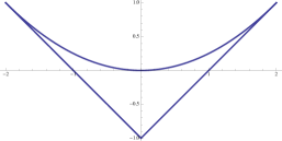
Figure 1. Domain $\Omega$

This is exactly the domain defined in (1.3).

We consider a family of weight functions defined on the domain $\Omega$ by

(3.3) $$W_{\gamma}(u,v)=2a_{w}^{\gamma}w(x)w(y)(u^{2}-4v)^{\gamma},\qquad(u,v)\in\Omega,$$

where the variables $(x,y)$ and $(u,v)$ are related by (3.2). The Jacobian of the change of variables (3.2) is given by $dudv=|x-y|dxdy$. Moreover, $u^{2}-4v=(x-y)^{2}$. It follows that

(3.4) $$\int_{\Omega}f(u,v)W_{\gamma}(u,v)dudv =2\int_{\triangle}f(x+y,xy)B_{\gamma}(x,y)dxdy$$

$$=\int_{[-1,1]^{2}}f(x+y,xy)B_{\gamma}(x,y)dxdy,$$

where the second equal sign follows since the integrant is a symmetric function of $x$ and $y$, and $[-1,1]^{2}$ is the union of $\triangle$ and its image under $(x,y)\mapsto(y,x)$. In particular, setting $f(x,y)=1$ shows that $W_{\gamma}$ is a normalized weight function.

In the case of $w(x)=w_{{\alpha},{\beta}}(x)$, the weight function $W_{\gamma}$ becomes $W_{{\alpha},{\beta},{\gamma}}$ in (1.2), which we restate below,

(3.5) $$W_{{\alpha},{\beta},{\gamma}}(u,v):=2a_{{\alpha},{\beta},{\gamma}}(1-u+v)^{\alpha}(1+u+v)^{\beta}(u^{2}-4v)^{\gamma},\quad(u,v)\in\Omega,$$

where the constant $a_{{\alpha},{\beta},{\gamma}}$ is given by [13, Lemma 6.1],

(3.6) $$a_{{\alpha},{\beta},{\gamma}}:=\frac{\sqrt{\pi}}{2^{2{\alpha}+2{\beta}+4{\gamma}+4}}\frac{\Gamma({\alpha}+{\beta}+{\gamma}+\frac{5}{2})\Gamma({\alpha}+{\beta}+2{\gamma}+3)}{\Gamma({\alpha}+1)\Gamma({\beta}+1)\Gamma({\gamma}+1)\Gamma({\alpha}+{\gamma}+\frac{3}{2})\Gamma({\beta}+{\gamma}+\frac{3}{2})},$$

which is the two-variable case of the Selberg integral (e.x., (1.1) of [5]). This weight function is integrable on $\Omega$ if ${\alpha},{\beta},{\gamma}>-1$ and ${\alpha}+{\gamma}+3/2>0$ and ${\beta}+{\gamma}+3/2>0$, and we assume that ${\alpha},{\beta},{\gamma}$ satisfy these inequalities from now on. Other examples of $W_{\gamma}$ include

$$e^{-au}(u^{2}-4v)^{\gamma}\quad\hbox{and}\quad e^{-a(u^{2}-2v)}(u^{2}-4v)^{\gamma},\quad a>0.$$

which correspond to the choices of $w(x)=e^{-ax}$ and $w(x)=e^{-ax^{2}}$.

Let ${\mathcal{N}}=\{(k,n):0\leq k\leq n\}$. In ${\mathcal{N}}$ define $(j,m)\prec(k,n)$ if $m<n$ or $j\leq k$ when $m=n$. Then the orthogonal polynomials $P_{k,n}^{({\gamma})}$ that satisfy

(3.7) $$P_{k,n}^{({\gamma})}(u,v)=u^{n-k}v^{k}+\sum_{(j,m)\prec(k,n)}a_{j,m}u^{m-j}v^{j}$$

and the orthogonality condition

(3.8) $$\int_{\Omega}P_{k,n}^{({\gamma})}(u,v)u^{m-j}v^{j}W_{{\gamma}}(u,v)dudv=0,\quad\forall(j,m)\prec(k,n),$$

are uniquely determined, as can be seen by the Gram-Schmidt process. The polynomials $P_{k,n}^{({\gamma})}$ are mutually orthogonal.

When $W_{\gamma}=W_{{\alpha},{\beta},{\gamma}}$, we denote these orthogonal polynomials by $P_{k,n}^{{\alpha},{\beta},{\gamma}}$.

In the case of ${\gamma}=\pm\frac{1}{2}$, these orthogonal polynomials can be given explicitly, as can be easily verified upon using (3.4). Let $p_{n}$ denote the orthogonal polynomial of degree $n$ with respect to $w$. Then an orthonormal basis with respect to $W_{-\frac{1}{2}}$ is given by

(3.9) $$P_{k,n}^{(-\frac{1}{2})}(u,v)=\frac{1}{\sqrt{2}}\begin{cases}p_{n}(x)p_{k}(y)+p_{n}(y)p_{k}(x),&0\leq k<n,\\ \sqrt{2}p_{n}(x)p_{n}(y),&k=n,\end{cases}$$

and an orthonormal basis with respect to $W_{\frac{1}{2}}$ is given by

(3.10) $$P_{k,n}^{(\frac{1}{2})}(u,v)=\sqrt{\frac{a_{w}^{-1/2}}{2a_{w}^{1/2}}}\,\frac{p_{n+1}(x)p_{k}(y)-p_{n+1}(y)p_{k}(x)}{x-y},\quad 0\leq k\leq n,$$

both families are defined under the mapping (3.2). It should be noted that the polynomials in (3.9) and (3.10) are normalized by their orthonormality, instead of by the leading coefficient as in (3.8), but they have the same structure as those in (3.8), so that the difference is just a constant multiple. In the case of $w=w_{{\alpha},{\beta}}$, the orthogonal polynomials in (3.9) and (3.10) are denoted by $P_{k,n}^{{\alpha},{\beta},-\frac{1}{2}}$ and $P_{k,n}^{{\alpha},{\beta},\frac{1}{2}}$, respectively, and they are expressed in terms of Jacobi polynomials $p_{n}^{({\alpha},{\beta})}$.

For $W_{{\alpha},{\beta},{\gamma}}$ these orthogonal polynomials were first studied by Koornwinder in [7], see also [8]. The above statements for more general weight function $W_{\gamma}$ are straightforward extensions and used in [12] for studying Gaussian cubature rules. Much more can be said about the orthogonal polynomials $P_{k,n}^{{\alpha},{\beta},{\gamma}}$. They are, for example, eigenfunctions of two differential operators of order 2 and order 4, respectively [7]. Another pair of differential operators were constructed in [13],

(3.11) $$\begin{split}&E_{-}^{{\alpha},{\beta}}:=u\frac{\partial^{2}}{\partial u^{2}}+2(v+1)\frac{\partial^{2}}{\partial u\partial v}+u\frac{\partial^{2}}{\partial v^{2}}+({\beta}-{\alpha})\frac{\partial}{\partial v}+({\alpha}+{\beta}+2)\frac{\partial}{\partial u}\\ &E_{+}^{{\alpha},{\beta},{\gamma}}:=\left[W_{{\alpha},{\beta},{\gamma}}(u,v)\right]^{-1}E_{-}^{-{\alpha},-{\beta}}W_{{\alpha},{\beta},{\gamma}+1}(u,v),\end{split}$$

and they act as raising and lowering operators on the orthogonal polynomials,

$$E_{-}^{{\alpha},{\beta}}P_{k,n}^{{\alpha},{\beta},{\gamma}}(u,v) =(n-k)(n+k+{\alpha}+{\beta}+1)P_{k,n-1}^{{\alpha},{\beta},{\gamma}+1}(u,v),$$

$$E_{+}^{{\alpha},{\beta},{\gamma}}P_{k,n-1}^{{\alpha},{\beta},{\gamma}+1}(u,v) =(n-k+2{\gamma}+1)(n+k+{\alpha}+{\beta}+2{\gamma}+2)P_{k,n}^{{\alpha},{\beta},{\gamma}}(u,v)$$

for $0\leq k\leq n-1$ and $E_{-}^{{\alpha},{\beta}}P_{n,n}^{{\alpha},{\beta},{\gamma}}(u,v)=0$. Together these two operators can be used to give a Rodrigues type formula for $P_{k,n}^{{\alpha},{\beta},{\gamma}}$ ([13, (5.1)]) and they can also be used to calculate the $L^{2}$-norms of $P_{k,n}^{{\alpha},{\beta},{\gamma}}$ and the coefficients in the recurrence relation.

The polynomials $P_{k,n}^{{\alpha},{\beta},{\gamma}}(u,v)$ also satisfy a quadratic transformation formula [13, Theorem 10.1] given by, for $0\leq k\leq n$,

(3.12) $$\begin{split}P_{n-k,n+k}^{{\alpha},{\alpha},{\gamma}}(u,v)&=2^{-n+k}P_{k,n}^{{\gamma},-\frac{1}{2},{\alpha}}(2v,u^{2}-2v-1),\\ u^{-1}P_{n-k,n+k+1}^{{\alpha},{\alpha},{\gamma}}(u,v)&=2^{-n+k}P_{k,n}^{{\gamma},\frac{1}{2},{\alpha}}(2v,u^{2}-2v-1).\end{split}$$

In particular, setting ${\gamma}=\pm\frac{1}{2}$ and ${\alpha}\mapsto{\gamma}$ and let $s=2xy$ and $t=x^{2}+y^{2}-1$, it follows that [13, p. 518],

(3.13) $$\begin{split}P_{k,n}^{-\frac{1}{2},-\frac{1}{2},{\gamma}}(s,t)&=c(p_{n+k}^{{\gamma},{\gamma}}(x)p_{n-k}^{{\gamma},{\gamma}}(y)+p_{n-k}^{{\gamma},{\gamma}}(x)p_{n+k}^{{\gamma},{\gamma}}(y)),\\ P_{k,n}^{\frac{1}{2},-\frac{1}{2},{\gamma}}(s,t)&=c(x-y)^{-1}\left[p_{n+k+1}^{{\gamma},{\gamma}}(x)p_{n-k}^{{\gamma},{\gamma}}(y)-p_{n-k}^{{\gamma},{\gamma}}(x)p_{n+k+1}^{{\gamma},{\gamma}}(x)\right],\\ P_{k,n}^{-\frac{1}{2},\frac{1}{2},{\gamma}}(s,t)&=c(x+y)^{-1}\left[p_{n+k+1}^{{\gamma},{\gamma}}(x)p_{n-k}^{{\gamma},{\gamma}}(y)+p_{n-k}^{{\gamma},{\gamma}}(x)p_{n+k+1}^{{\gamma},{\gamma}}(x)\right],\\ P_{k,n}^{\frac{1}{2},\frac{1}{2},{\gamma}}(s,t)&=c(x^{2}-y^{2})^{-1}\left[p_{n+k+2}^{{\gamma},{\gamma}}(x)p_{n-k}^{{\gamma},{\gamma}}(y)-p_{n-k}^{{\gamma},{\gamma}}(x)p_{n+k+2}^{{\gamma},{\gamma}}(x)\right],\end{split}$$

where $c$ is a constant proportional to $2^{n-k}$. In other words, a basis of orthogonal polynomials for $W_{\pm\frac{1}{2},\pm\frac{1}{2},{\gamma}}$ can be explicitly given in terms of Jacobi polynomials.

For further results on $P_{k,n}^{{\alpha},{\beta},{\gamma}}$, including explicit series expansions and recursive relations, see [7, 9, 13].

It is worth to mention that the relation (3.4) shows that orthogonal polynomials $P_{k,n}$ for $W_{\gamma}$ are closely related to the orthogonal polynomials with respect to $B_{\gamma}$ on $[-1,1]^{2}$, as seen by

$$W_{\gamma}(x+y,xy)=B_{\gamma}(x,y)|x-y|$$

and (3.4). Indeed, if $R_{k,n}$ is polynomial orthogonal to $x^{l}y^{m}$, if $\max\{l,m\}<n$, with respect to $B_{\gamma}$ on $[-1,1]^{2}$, then $R_{k,n}(x,y)+R_{k,n}(y,x)$ is a symmetric polynomial orthogonal to $x^{l}y^{m}+x^{m}y^{l}$, if $\max\{l,m\}<n$, for $B_{\gamma}$ since $B_{\gamma}$ is symmetric. Hence, under the bijection (3.2), the polynomial

$$P_{k,n}(u,v):=R_{k,n}(x,y)+R_{k,n}(y,x)$$

is an orthogonal polynomial with respect to $W_{\gamma}$ on $\Omega$. Since the mapping (3.2) is not linear, one needs to be careful about the degree of $P_{k,n}$. In the case of $w=w_{{\alpha},{\beta}}$, the symmetric orthogonal polynomials for $B_{\gamma}$ are the $BC_{2}$ type polynomials, the precursor of the generalized Jacobi polynomials of $BC_{n}$ type.

3.2. Reproducing kernel

Recall that $K_{n}(W_{\gamma};\cdot,\cdot)$ denotes the reproducing kernel of $\Pi_{n}^{2}$ in $L^{2}(W_{\gamma})$, which we shall denote by $K_{n}^{({\gamma})}(\cdot,\cdot)$ below. In contrast to (2.5), we derive a closed formula for $K_{n}^{({\gamma})}(\cdot,\cdot)$ in the case of ${\gamma}=\pm\frac{1}{2}$ in this subsection.

Theorem 3.1.

Let $k_{n}(\cdot,\cdot):=k_{n}(w;\cdot,\cdot)$ be the kernel defined in (2.1). Set

$$u:=(u_{1},u_{2})=(x_{1}+x_{2},x_{1}x_{2})\quad\hbox{and}\quad v:=(v_{1},v_{2})=(y_{1}+y_{2},y_{1}y_{2}).$$

Then the reproducing kernel $K_{n}^{(-\frac{1}{2})}(\cdot,\cdot)$ for $W_{-\frac{1}{2}}$ is given by

(3.14) $$K_{n}^{(-\frac{1}{2})}(u,v)=\frac{1}{2}\left[k_{n}(x_{1},y_{1})k_{n}(x_{2},y_{2})+k_{n}(x_{2},y_{1})k_{n}(x_{1},y_{2})\right],$$

and the reproducing kernel $K_{n}^{(\frac{1}{2})}(\cdot,\cdot)$ for $W_{\frac{1}{2}}$ is given by

(3.15) $$K_{n}^{(\frac{1}{2})}(u,v)=\frac{1}{2}\frac{k_{n+1}(x_{1},y_{1})k_{n+1}(x_{2},y_{2})-k_{n+1}(x_{2},y_{1})k_{n+1}(x_{1},y_{2})}{(x_{1}-x_{2})(y_{1}-y_{2})}.$$

Proof.

Denote the right hand side of (3.14) by $\widehat{k}_{n}((x_{1},x_{2}),(y_{1},y_{2}))$. By the definition of $k_{n}(\cdot,\cdot)$ in (2.1), for a fixed $y_{1},y_{2}$, we have

$$\widehat{k}_{n}((x_{1},x_{2}),(y_{1},y_{2}))=\frac{1}{2}\sum_{k=0}^{n}\sum_{j=0}^{n}p_{k}(y_{1})p_{j}(y_{1})\left[p_{k}(x_{1})p_{j}(x_{2})+p_{k}(x_{2})p_{j}(x_{1})\right],$$

which shows, upon setting $u_{1}=x_{1}+x_{2}$, $u_{2}=x_{1}x_{2}$, that $\widehat{k}_{n}((x_{1},x_{2}),(y_{1},y_{2}))$ is a polynomial of degree $n$ in $(u_{1},y_{2})$. Hence, if we define $\widehat{K}_{n}((u_{1},u_{2}),(v_{1},v_{2}))=\widehat{k}_{n}((x_{1},x_{2}),(y_{1},y_{2}))$ under the mapping $(u_{1},u_{2})\mapsto(x_{1}+x_{2},x_{1}x_{2})$ and $(v_{1},v_{2})\mapsto(y_{1}+y_{2},y_{1}y_{2})$, then $\widehat{K}$ is a polynomial of degree $n$ in $(u_{1},u_{2})$ and, by symmetry, in $(v_{1},v_{2})$. Thus, we only have to verify the reproducing property. For $0\leq j\leq m\leq n$, the reproducing property of $k_{n}(\cdot,\cdot)$ implies immediately

$$\int_{\Omega}\widehat{K}_{n}((u_{1},u_{2}),(v_{1},v_{2}))P_{j,m}^{(-\frac{1}{2})}(v_{1},v_{2})W_{-\frac{1}{2}}(v_{1},v_{2})dv_{1}dv_{2}$$

$$= \int_{[-1,1]^{2}}\widehat{k}_{n}((x_{1},x_{2}),(y_{1},y_{2}))P_{j,m}^{(-\frac{1}{2})}(y_{1}+y_{2},y_{1}y_{2})w(y_{1})w(y_{2})dy_{1}dy_{2}$$

$$= \,\frac{1}{\sqrt{2}}\left[p_{m}(x_{1})p_{j}(x_{2})+p_{j}(x_{1})p_{m}(x_{2})\right]=P_{j,m}^{(-\frac{1}{2})}(u_{1},u_{2}),$$

which shows that $\widehat{K}_{n}((u_{1},u_{2}),(v_{1},v_{2}))$ is the reproducing kernel of $\Pi_{n}^{2}$, so that (3.14) holds.

Denote now the right hand side of (3.15) by $\widehat{k}_{n}((x_{1},x_{2}),(y_{1},y_{2}))$. Then, for fixed $(y_{1},y_{2})$, it is easy to see that

$$\widehat{k}_{n}((x_{1},x_{2}),(y_{1},y_{2}))=\sum_{j=0}^{n+1}\sum_{k=0}^{n+1}\frac{p_{j}(y_{1})p_{k}(y_{2})}{y_{1}-y_{2}}\frac{p_{j}(x_{1})p_{k}(x_{2})-p_{j}(x_{2})p_{k}(x_{1})}{x_{1}-x_{2}},$$

which shows, since the terms for $k=j$ are zero, that $\widehat{k}_{n}((x_{1},x_{2}),(y_{1},y_{2}))$ is a polynomial of degree $n$ in $(u_{1},u_{2})$, where $u_{1}=x_{1}+x_{2}$ and $u_{2}=x_{1}x_{2}$. By symmetry, the same holds for $(y_{1},y_{2})$ with $(x_{1},x_{2})$ fixed. Thus, it remains to prove the reproducing property, which works similarly as in the case of ${\gamma}=-1/2$ upon using the fact that $(y_{1}-y_{2})^{2}$ in $W_{\frac{1}{2}}(u_{1},u_{2})=(y_{1}-y_{2})^{2}w(y_{1})w(y_{2})$ cancels the denominators in both $\widehat{k}_{n}(\cdot,\cdot)$ and $P_{j,m}^{\frac{1}{2}}(y_{1}+y_{2},y_{1}y_{2})$. ∎

The closed formula for the reproducing kernel allows us to study the convergence of the Fourier orthogonal expansions, which will be discussed in Section 5.

4. Orthogonal polynomials for weight functions on $[-1,1]^{2}$

In this section we study orthogonal polynomials for the family of weight functions defined in (3.3) on $[-1,1]^{2}$, which are closely related to $W_{\gamma}$. The orthogonal polynomials are given in the first subsection, their further properties are in the second subsection, and a compact formula for the reproducing kernel is in the third subsection.

4.1. Orthogonal polynomials

Let $w$ be the weight function on $[-1,1]$ and let $W_{\gamma}$ be the weight function defined in (3.3). We then define

(4.1) $${\mathcal{W}}_{\gamma}(x,y):=W_{\gamma}(2xy,x^{2}+y^{2}-1)|x^{2}-y^{2}|,\qquad(x,y)\in[-1,1]^{2},$$

which is the quadratic transform that has appeared in (3.12). Let $\Omega$ be the domain (1.3) of $W_{\gamma}$. The fact that $(x,y)\in[-1,1]^{2}$ implies that $(2xy,x^{2}+y^{2}-1)\in\Omega$ is shown in the lemma below. In the case that $W_{\gamma}=W_{{\alpha},{\beta},{\gamma}}$, the weight function ${\mathcal{W}}_{\gamma}$ becomes, up to a constant, ${\mathcal{W}}_{{\alpha},{\beta},{\gamma}}$ defined in (1.1), which we restate as,

(4.2) $${\mathcal{W}}_{{\alpha},{\beta},{\gamma}}(x,y):=2a_{{\alpha},{\beta},{\gamma}}4^{\gamma}|x-y|^{2{\alpha}+1}|x+y|^{2{\beta}+1}(1-x^{2})^{\gamma}(1-y^{2})^{\gamma},$$

where ${\alpha},{\beta},{\gamma}>-1$, ${\alpha}+{\gamma}+\frac{1}{2}>-1$ and ${\beta}+{\gamma}+\frac{1}{2}>-1$. These conditions on the parameters, ensuring the integrability of ${\mathcal{W}}_{{\alpha},{\beta},{\gamma}}$, are the same as those for $W_{{\alpha},{\beta},{\gamma}}$. The weight function ${\mathcal{W}}_{\gamma}$, and ${\mathcal{W}}_{{\alpha},{\beta},{\gamma}}$, is normalized as shown below. We define a region $\Omega^{*}:=\{(x,y):-1<x<y<1\}$.

Lemma 4.1.

The mapping $(x,y)\mapsto(2xy,x^{2}+y^{2}-1)$ is a bijection from $\Omega^{*}$ onto $\Omega$. Furthermore,

(4.3) $$\int_{\Omega}f(u,v)W_{{\gamma}}(u,v)dudv=\int_{[-1,1]^{2}}f(2xy,x^{2}+y^{2}-1){\mathcal{W}}_{{\gamma}}(x,y)dxdy.$$

Proof.

For $(x,y)\in[-1,1]^{2}$, let us write $x=\cos{\theta}$ and $y=\cos\phi$, $0\leq{\theta},\phi\leq\pi$. Then it is easy to see that

(4.4) $$2xy=\cos({\theta}-\phi)+\cos({\theta}+\phi),\quad x^{2}+y^{2}-1=\cos({\theta}-\phi)\cos({\theta}+\phi),$$

from which it follows readily that $(2xy,x^{2}+y^{2}-1)\in\Omega$. For the change of variable $u=2xy$ and $v=x^{2}+y^{2}-1$, we have $dudv=4|x^{2}-y^{2}|dxdy$, from which the stated formula follows. ∎

As a more general example, we consider $w$ being a generalized Jacobi weight.

Lemma 4.2.

Let $w\in GJ$ be defined as in (2.3). Then

(4.5) $${\mathcal{W}}_{{\gamma}}(x,y)=\Psi(x,y)|x-y|^{2{\gamma}_{0}+1} \prod_{k=1}^{r}\left|1+t_{k}^{2}-(x-t_{k})^{2}-(y-t_{k})^{2}\right|^{{\gamma}_{k}}$$

$$\qquad\times|x+y|^{2{\gamma}_{r+1}+1}(1-x^{2})^{\gamma}(1-y^{2})^{\gamma},$$

where $\Psi(\cos{\theta},\cos\phi)=\psi(\cos({\theta}-\phi))\psi(\cos({\theta}+\phi))$.

We consider orthogonal polynomials with respect to the inner product

(4.6) $${\langle}f,g{\rangle}_{{\mathcal{W}}_{\gamma}}:=\int_{[-1,1]^{2}}f(x,y)g(x,y){\mathcal{W}}_{\gamma}(x,y)dxdy.$$

Let ${\mathcal{V}}_{n}({\mathcal{W}}_{{\gamma}})$ denote the space of orthogonal polynomials of degree $n$ with respect to the inner product ${\langle}\cdot,\cdot{\rangle}_{{\mathcal{W}}_{\gamma}}$. It turns out that a basis of ${\mathcal{V}}_{n}({\mathcal{W}}_{{\gamma}})$ can be expressed in terms of orthogonal polynomials with respect to $W_{{\gamma}}$ and three other related weight functions. Recall that ${\langle}\cdot,\cdot{\rangle}_{W}$ is defined in (2.4). We define three other weight functions

(4.7) $$\begin{split}W_{\gamma}^{(1,1)}(u,v)&:=2a_{w^{(1,1)}}^{\gamma}(1-u+v)(1+u+v)W_{\gamma}(u,v),\\ W_{\gamma}^{(1,0)}(u,v)&:=2a_{w^{(1,0)}}^{\gamma}(1-u+v)W_{\gamma}(u,v),\\ W_{\gamma}^{(0,1)}(u,v)&:=2a_{w^{(0,1)}}^{\gamma}(1+u+v)W_{\gamma}(u,v),\end{split}\quad(u,v)\in\Omega,$$

where we define

(4.8) $$w^{(i,j)}(x):=(1-x)^{i}(1+x)^{j}w(x),\quad i,j=0,1.$$

Under the change of variables $u=x+y$ and $v=xy$, $1-u+v=(1-x)(1-y)$ and $1+u+v=(1+x)(1+y)$. The three weight functions in (4.7) are normalized so that $\int_{\Omega}W_{\gamma}^{i,j}(u,v)dudv=1$. Clearly these three weight functions are of the same type as $W_{\gamma}$.

In the following theorem, we denote by $\{P_{k,n}^{({\gamma})}:0\leq k\leq n\}$ an orthonormal basis of ${\mathcal{V}}_{n}(W_{{\gamma}})$ under ${\langle}\cdot,\cdot{\rangle}_{W_{{\gamma}}}$. For $0\leq k\leq n$, we further denote by $P_{k,n}^{({\gamma}),1,1}$, $P_{k,n}^{({\gamma}),1,0,}$, $P_{k,n}^{({\gamma}),0,1}$ the orthonormal polynomials of degree $n$ with respect to ${\langle}f,g{\rangle}_{W}$ for $W=W_{\gamma}^{(1,1)}$, $W_{\gamma}^{(1,0)}$, $W_{\gamma}^{(0,1)}$, respectively.

Theorem 4.3.

For $n=0,1,\ldots$, an orthonormal basis of ${\mathcal{V}}_{2n}({\mathcal{W}}_{{\gamma}})$ is given by

(4.9) $$\begin{split}{}_{1}Q_{k,2n}^{({\gamma})}(x,y):=&P_{k,n}^{({\gamma})}(2xy,x^{2}+y^{2}-1),\qquad 0\leq k\leq n,\\ {}_{2}Q_{k,2n}^{({\gamma})}(x,y):=&b_{\gamma}^{(1,1)}(x^{2}-y^{2})P_{k,n-1}^{({\gamma}),1,1}(2xy,x^{2}+y^{2}-1),\quad 0\leq k\leq n-1,\end{split}$$

and an orthonormal basis of ${\mathcal{V}}_{2n+1}({\mathcal{W}}_{{\gamma}})$ is given by

(4.10) $$\begin{split}&{}_{1}Q_{k,2n+1}^{({\gamma})}(x,y):=b_{\gamma}^{(0,1)}(x+y)P_{k,n}^{({\gamma}),0,1}(2xy,x^{2}+y^{2}-1),\qquad 0\leq k\leq n,\\ &{}_{2}Q_{k,2n+1}^{({\gamma})}(x,y):=b_{\gamma}^{(1,0)}(x-y)P_{k,n}^{({\gamma}),1,0}(2xy,x^{2}+y^{2}-1),\qquad 0\leq k\leq n,\end{split}$$

where $b_{\gamma}^{(i,j)}:=\sqrt{a^{\gamma}_{w^{(i,j)}}/a^{\gamma}_{w}}$ for $i,j=0,1$.

Proof.

These polynomials evidently form a basis if they are orthogonal. By Lemma 4.1, for $0\leq j\leq m$ and $0\leq k\leq n$,

$$\left\langle{}_{1}Q_{k,2n}^{({\gamma})},{}_{1}Q_{j,2m}^{({\gamma})}\right\rangle_{{\mathcal{W}}_{{\gamma}}}={\langle}P_{k,n}^{({\gamma})},P_{j,m}^{({\gamma})}{\rangle}_{W_{\gamma}}=\delta_{k,j}\delta_{n,m},$$

and, setting $F=P_{k,n-1}^{({\gamma}),1,1}P_{k,n}^{({\gamma})}$,

$$\left\langle{}_{1}Q_{k,2n}^{({\gamma})},{}_{2}Q_{j,2m}^{({\gamma})}\right\rangle_{{\mathcal{W}}_{{\gamma}}}=\int_{[-1,1]^{2}}(x^{2}-y^{2})F(2xy,x^{2}+y^{2}-1){\mathcal{W}}_{{\gamma}}(x,y)dxdy.$$

The right hand side of the above equation changes sign under the change of variables $(x,y)\mapsto(y,x)$, which shows that $\left\langle{}_{1}Q_{k,2n}^{({\gamma})},{}_{2}Q_{j,2m}^{({\gamma})}\right\rangle_{{\mathcal{W}}_{{\gamma}}}=0$. Moreover, since $(x^{2}-y^{2})^{2}{\mathcal{W}}_{{\gamma}}(x,y)dxdy$ is equal to a constant multiple of $W_{{\gamma}}^{(1,1)}(u,v)dudv$, we see that

$$\left\langle{}_{2}Q_{k,2n}^{({\gamma})},{}_{2}Q_{j,2m}^{({\gamma})}\right\rangle_{{\mathcal{W}}_{{\gamma}}}=\left\langle P_{k,n-1}^{({\gamma}),1,1},P_{j,m-1}^{({\gamma}),1,1}\right\rangle_{W_{\gamma}^{(1,1)}}=\delta_{k,j}\delta_{n,m}.$$

Furthermore, setting $F=P_{k,n}^{({\gamma})}P_{k,n}^{({\gamma}),0,1}$, we obtain

$$\left\langle{}_{1}Q_{k,2n}^{({\gamma})},{}_{1}Q_{j,2m+1}^{({\gamma})}\right\rangle_{{\mathcal{W}}_{{\gamma}}}=\int_{[-1,1]^{2}}(x+y)G(2xy,x^{2}+y^{2}-1){\mathcal{W}}_{{\gamma}}(x,y)dxdy,$$

which is equal to zero since the right hand side changes sign under $(x,y)\mapsto(-x,-y)$. The same proof shows also $\left\langle{}_{1}Q_{k,2n}^{({\gamma})},{}_{2}Q_{j,2m+1}^{({\gamma})}\right\rangle_{{\mathcal{W}}_{{\gamma}}}=0$. Together, we have proved the orthogonality of ${}_{1}Q_{k,2n}^{({\gamma})}$ and ${}_{2}Q_{k,2n}^{({\gamma})}$.

Since $(x-y)(x+y)=x^{2}-y^{2}$ changes sign under $(x,y)\mapsto(y,x)$, the same consideration shows that $\left\langle{}_{1}Q_{k,2n+1}^{({\gamma})},{}_{2}Q_{j,2m+1}^{({\gamma})}\right\rangle_{{\mathcal{W}}_{{\gamma}}}=0$. Finally, we also have

$$\left\langle{}_{1}Q_{k,2n+1}^{({\gamma})},{}_{1}Q_{j,2m+1}^{({\gamma})}\right\rangle_{{\mathcal{W}}_{{\gamma}}}=\left\langle P_{k,n}^{({\gamma}),0,1},P_{j,m}^{({\gamma}),0,1}\right\rangle_{W_{{\gamma}}^{(0,1)}}=\delta_{k,j}\delta_{n,m}$$

$$\left\langle{}_{2}Q_{k,2n+1}^{({\gamma})},{}_{2}Q_{j,2m+1}^{({\gamma})}\right\rangle_{{\mathcal{W}}_{{\gamma}}}=\left\langle P_{k,n}^{({\gamma}),1,0},P_{j,m}^{({\gamma}),1,0}\right\rangle_{W_{{\gamma}}^{(1,0)}}=\delta_{k,j}\delta_{n,m},$$

which proves the orthogonality of ${}_{1}Q_{k,2n+1}^{({\gamma})}$ and ${}_{2}Q_{k,2n+1}^{({\gamma})}$. ∎

For the weight function ${\mathcal{W}}_{{\alpha},{\beta},{\gamma}}$, we denote a basis of orthonormal polynomials by $P_{k,n}^{{\alpha},{\beta},{\gamma}}$ in the following theorem.

Theorem 4.4.

For $n=0,1,\ldots$, an orthonormal basis of ${\mathcal{V}}_{2n}({\mathcal{W}}_{{\alpha},{\beta},{\gamma}})$ is given by

(4.11) $$\begin{split}{}_{1}Q_{k,2n}^{{\alpha},{\beta},{\gamma}}(x,y):=&P_{k,n}^{{\alpha},{\beta},{\gamma}}(2xy,x^{2}+y^{2}-1),\qquad 0\leq k\leq n,\\ {}_{2}Q_{k,2n}^{{\alpha},{\beta},{\gamma}}(x,y):=&b_{{\alpha},{\beta},{\gamma}}^{(1,1)}(x^{2}-y^{2})P_{k,n-1}^{{\alpha}+1,{\beta}+1,{\gamma}}(2xy,x^{2}+y^{2}-1),\,\,0\leq k\leq n-1,\end{split}$$

and an orthonormal basis of ${\mathcal{V}}_{2n+1}({\mathcal{W}}_{{\alpha},{\beta},{\gamma}})$ is given by

(4.12) $$\begin{split}&{}_{1}Q_{k,2n+1}^{{\alpha},{\beta},{\gamma}}(x,y):=b_{{\alpha},{\beta},{\gamma}}^{(0,1)}(x+y)P_{k,n}^{{\alpha},{\beta}+1,{\gamma}}(2xy,x^{2}+y^{2}-1),\quad 0\leq k\leq n,\\ &{}_{2}Q_{k,2n+1}^{{\alpha},{\beta},{\gamma}}(x,y):=b_{{\alpha},{\beta},{\gamma}}^{(1,0)}(x-y)P_{k,n}^{{\alpha}+1,{\beta},{\gamma}}(2xy,x^{2}+y^{2}-1),\quad 0\leq k\leq n,\end{split}$$

where $b_{{\alpha},{\beta},{\gamma}}^{(i,j)}:=\sqrt{a_{{\alpha}+i,{\beta}+j,{\gamma}}/a_{{\alpha},{\beta},{\gamma}}}$ for $i,j=0,1$.

4.2. Special cases and properties

In the case of ${\gamma}=\pm\frac{1}{2}$, we can derive an explicit formula for the basis from (3.9) and (3.10), which takes a particularly simple form if we change variables to

(4.13) $$x=\cos\theta,\quad y=\cos\phi,\quad 0\leq{\theta},\phi\leq\pi.$$

Corollary 4.5.

For ${\gamma}=\pm\frac{1}{2}$, the orthonormal basis defined in (4.9) and (4.10) of ${\mathcal{V}}_{n}({\mathcal{W}}_{\pm\frac{1}{2}})$ satisfies, under (4.13), explicit formulas upon using the relations

(4.14) $$P_{k,n}^{(-\frac{1}{2})}(2xy,x^{2}+y^{2}-1)$$

$$\quad=\frac{1}{\sqrt{2}}\left[p_{n}(\cos({\theta}-\phi))p_{k}(\cos({\theta}+\phi))+p_{k}(\cos({\theta}-\phi))p_{n}(\cos({\theta}+\phi))\right]$$

for $0\leq k\leq n$, where the $k=n$ term $P_{n,n}^{(-\frac{1}{2})}$ is multiplied by the constant $\sqrt{2}$; furthermore, for $0\leq k\leq n$,

(4.15) $$P_{k,n}^{(\frac{1}{2})}(2xy,x^{2}+y^{2}-1)$$

$$=\sqrt{\frac{a_{w}^{-1/2}}{2a_{w}^{1/2}}}\,\frac{p_{n}(\cos({\theta}-\phi))p_{k}(\cos({\theta}+\phi))-p_{k}(\cos({\theta}-\phi))p_{n}(\cos({\theta}+\phi))}{2\sin{\theta}\sin\phi}.$$

Proof.

This follows immediately from (4.4), (3.9) and (3.10). ∎

In particular, the orthonormal basis for the weight function

$${\mathcal{W}}_{{\alpha},{\beta},\pm\frac{1}{2}}(x_{1},x_{2})=c|x_{1}-x_{2}|^{2{\alpha}+1}|x_{1}+x_{2}|^{2{\beta}+1}(1-x_{1}^{2})^{\pm\frac{1}{2}}(1-x_{2}^{2})^{\pm\frac{1}{2}}$$

on $[-1,1]^{2}$, where $c=2a_{a,{\beta},\pm\frac{1}{2}}4^{\pm\frac{1}{2}}$, can be given in terms of the Jacobi polynomials.

Proposition 4.6.

Let ${\alpha},{\beta}>-1$. An orthonormal basis of ${\mathcal{V}}_{2n}({\mathcal{W}}_{{\alpha},{\beta},-\frac{1}{2}})$ is given by, for $0\leq k\leq n$ and $0\leq k\leq n-1$, respectively,

$${}_{1}Q_{k,2n}^{({\alpha},{\beta},-\frac{1}{2})}(\cos{\theta},\cos\phi)=\frac{1}{\sqrt{2}}\left[p_{n}^{({\alpha},{\beta})}(\cos({\theta}-\phi))p_{k}^{({\alpha},{\beta})}(\cos({\theta}+\phi))\right.$$

$$\qquad\qquad\qquad\qquad\qquad\qquad\qquad\left.+p_{k}^{({\alpha},{\beta})}(\cos({\theta}-\phi))p_{n}^{({\alpha},{\beta})}(\cos({\theta}+\phi))\right],$$

$${}_{2}Q_{k,2n}^{({\alpha},{\beta},-\frac{1}{2})}(\cos{\theta},\cos\phi)=\frac{b_{{\alpha},{\beta},-\frac{1}{2}}^{(1,1)}}{\sqrt{2}}(x^{2}-y^{2})\left[p_{n-1}^{({\alpha}+1,{\beta}+1)}(\cos({\theta}-\phi))p_{k}^{({\alpha}+1,{\beta}+1)}(\cos({\theta}+\phi))\right.$$

$$\qquad\qquad\qquad\qquad\qquad\qquad\qquad\left.+p_{k}^{({\alpha}+1,{\beta}+1)}(\cos({\theta}-\phi))p_{n-1}^{({\alpha}+1,{\beta}+1)}(\cos({\theta}+\phi))\right],$$

and an orthonormal basis of ${\mathcal{V}}_{2n+1}({\mathcal{W}}_{{\alpha},{\beta},-\frac{1}{2}})$ is given by, for $0\leq k\leq n$,

$${}_{1}Q_{k,2n+1}^{({\alpha},{\beta},-\frac{1}{2})}(\cos{\theta},\cos\phi)=\frac{b_{{\alpha},{\beta},-\frac{1}{2}}^{(0,1)}}{\sqrt{2}}(x+y)\left[p_{n}^{({\alpha},{\beta}+1)}(\cos({\theta}-\phi))p_{k}^{({\alpha},{\beta}+1)}(\cos({\theta}+\phi))\right.$$

$$\qquad\qquad\qquad\qquad\qquad\qquad\qquad\left.+p_{k}^{({\alpha},{\beta}+1)}(\cos({\theta}-\phi))p_{n}^{({\alpha},{\beta}+1)}(\cos({\theta}+\phi))\right],$$

$${}_{2}Q_{k,2n+1}^{({\alpha},{\beta},-\frac{1}{2})}(\cos{\theta},\cos\phi)=\frac{b_{{\alpha},{\beta},-\frac{1}{2}}^{(1,0)}}{\sqrt{2}}(x-y)\left[p_{n}^{({\alpha}+1,{\beta})}(\cos({\theta}-\phi))p_{k}^{({\alpha}+1,{\beta})}(\cos({\theta}+\phi))\right.$$

$$\qquad\qquad\qquad\qquad\qquad\qquad\qquad\left.+p_{k}^{({\alpha}+1,{\beta})}(\cos({\theta}-\phi))p_{n}^{({\alpha}+1,{\beta})}(\cos({\theta}+\phi))\right],$$

where whenever $k=n$ the polynomial needs to be multiplied by an additional $\sqrt{2}$.

Similarly, an orthonormal basis for ${\mathcal{V}}_{n}({\mathcal{W}}_{{\alpha},{\beta},\frac{1}{2}})$ can be given explicitly in terms of the Jacobi polynomials upon using (4.15).

By Theorem 4.3, the orthogonal polynomials for ${\mathcal{W}}_{{\alpha},{\beta},{\gamma}}$ are expressed in terms of orthogonal polynomials for $W_{{\alpha},{\beta},{\gamma}}$, which in turn are expressed in terms of the symmetric orthogonal polynomials with respect to the weight function

$$B_{{\alpha},{\beta},{\gamma}}(x,y)=(1-x)^{\alpha}(1+x)^{\beta}(1-y)^{\alpha}(1+y)^{\beta}|x-y|^{2{\gamma}+1}$$

on $[-1,1]^{2}$; see (3.1) with $w=w_{{\alpha},{\beta}}$ and the remark at the end of Subsection 3.1. Both weight functions ${\mathcal{W}}_{{\alpha},{\beta},{\gamma}}$ and $B_{{\alpha},{\beta},{\gamma}}$ are defined on $[-1,1]^{2}$, and they satisfy

(4.16) $${\mathcal{W}}_{{\alpha},-\frac{1}{2},{\gamma}}(x,y)=4^{\gamma}B_{{\gamma},{\gamma},{\alpha}}(x,y).$$

Consequently, there is some kind of automorphism among these orthogonal polynomials. By Theorem 4.4, symmetric orthogonal polynomials with respect to ${\mathcal{W}}_{{\gamma},-\frac{1}{2},{\alpha}}$ are given by, for $0\leq k\leq n$,

$$P_{k,n}^{{\gamma},-\frac{1}{2},{\alpha}}(2xy,x^{2}+y^{2}-1)\quad\hbox{and}\quad(x+y)P_{k,n}^{{\gamma},\frac{1}{2},{\alpha}}(2xy,x^{2}+y^{2}-1)$$

of degree $2n$ and $2n+1$, respectively. These are, by (4.16), symmetric orthogonal polynomials for $B_{{\alpha},{\alpha},{\gamma}}$, from which we can derive orthogonal polynomials for $W_{{\alpha},{\alpha},{\gamma}}$ by a change of variables $u=x+y$ and $v=xy$ as shown in the end of Subsection 3.1. Since $x^{2}+y^{2}=u^{2}-2v$, we see that

$$P_{k,n}^{{\gamma},-\frac{1}{2},{\alpha}}(2v,u^{2}-2v-1)\quad\hbox{and}\quad u_{1}P_{k,n}^{{\gamma},\frac{1}{2},{\alpha}}(2v,u^{2}-2v-1)$$

are orthogonal polynomials with respect to $W_{{\alpha},{\alpha},{\gamma}}$ of degree $k+n$. Comparing the leading coefficients by (3.7), we conclude that

$$P_{k,n}^{{\gamma},-\frac{1}{2},{\alpha}}(2v,u^{2}-2v-1) =2^{n-k}P_{n-k,n+k}^{{\alpha},{\alpha},{\gamma}}(u,v),$$

$$uP_{k,n}^{{\gamma},\frac{1}{2},{\alpha}}(2v,u^{2}-2v-1) =2^{n-k}P_{n-k,n+k}^{{\alpha},{\alpha},{\gamma}}(u,v).$$

These are, however, precisely (3.12). These relations translate to orthogonal polynomials with respect to ${\mathcal{W}}_{{\alpha},{\beta},{\gamma}}$ on $[-1,1]^{2}$ as follows. Let ${}_{i}Q_{k,n}^{{\alpha},{\beta},{\gamma}}$ denote the orthogonal polynomials given in (4.9) and (4.10) but with $P_{k,n}^{{\alpha},{\beta},{\gamma}}$ as the monic orthogonal polynomial as in (3.7).

Proposition 4.7.

We have the following quadratic transforms, for $0\leq k\leq\lfloor\frac{n}{2}\rfloor$,

$${}_{1}Q_{k,n}^{{\gamma},-1/2,{\alpha}}(\cos{\theta},\cos\phi)=2^{\lfloor\frac{n}{2}\rfloor-k}{}_{1}Q_{\lfloor\frac{n}{2}\rfloor-k,2n-2\lfloor\frac{n}{2}\rfloor+2k}^{{\alpha},{\alpha},{\gamma}}\left(\cos\tfrac{{\theta}-\phi}{2},\cos\tfrac{{\theta}+\phi}{2}\right),$$

$$\sin{\theta}\sin\phi\,{}_{2}Q_{k,n}^{{\gamma},-1/2,{\alpha}}(\cos{\theta},\cos\phi)$$

$$\quad=2^{\lfloor\frac{n+1}{2}\rfloor-k}\sin\tfrac{{\theta}-\phi}{2}\sin\tfrac{{\theta}+\phi}{2}\times{}_{2}Q_{\lfloor\frac{n-1}{2}\rfloor-k,2n-2\lfloor\frac{n+1}{2}\rfloor+2k}^{{\alpha},{\alpha},{\gamma}}\left(\cos\tfrac{{\theta}-\phi}{2},\cos\tfrac{{\theta}+\phi}{2}\right).$$

Proof.

From the quadratic transform formulas satisfied by $P_{k,n}^{{\alpha},{\beta},{\gamma}}(u_{1},u_{2})$, we have

(4.17) $$\begin{split}P_{n-k,n+k}^{{\alpha},{\alpha},{\gamma}}(x+y,xy)&=2^{-n+k}P_{k,n}^{{\gamma},-\frac{1}{2},{\alpha}}(2xy,x^{2}+y^{2}-1),\\ (x+y)^{-1}P_{n-k,n+k+1}^{{\alpha},{\alpha},{\gamma}}(x+y,xy)&=2^{-n+k}P_{k,n}^{{\gamma},\frac{1}{2},{\alpha}}(2xy,x^{2}+y^{2}-1).\end{split}$$

If $x=\cos\theta$ and $y=\cos\phi$, then it is easy to see that

$$x+y=2\cos\tfrac{{\theta}-\phi}{2}\cos\tfrac{{\theta}+\phi}{2},\quad xy=\cos^{2}\tfrac{{\theta}-\phi}{2}+\cos^{2}\tfrac{{\theta}+\phi}{2}-1$$

Consequently, the equations for ${}_{1}Q_{k,2m}^{{\gamma},-1/2,{\alpha}}$ and ${}_{1}Q_{k,2m+1}^{{\gamma},-1/2,{\alpha}}$ follow immediately from (4.17), (4.11) and (4.12). For ${}_{2}Q_{k,2m}^{{\gamma},-1/2,{\alpha}}$ and ${}_{2}Q_{k,2m+1}^{{\gamma},-1/2,{\alpha}}$ we use in addition the trigonometric identities $\cos{\theta}-\cos\phi=2\sin\tfrac{{\theta}-\phi}{2}\sin\tfrac{{\theta}+\phi}{2}$ and $\cos^{2}\tfrac{{\theta}-\phi}{2}-\cos^{2}\tfrac{{\theta}+\phi}{2}=\sin{\theta}\sin\phi$. ∎

In the case of ${\alpha}={\beta}=-1/2$, the weight function becomes

$${\mathcal{W}}_{-\frac{1}{2},-\frac{1}{2},{\gamma}}(x,y)=(1-x^{2})^{\gamma}(1-y^{2})^{\gamma},\quad(x,y)\in[-1,1]^{2},$$

which is the product Gegenbauer weight function. An orthonormal basis of ${\mathcal{V}}_{n}^{d}$ for this weight function is usually given by the product Jacobi polynomials

$$P_{k,n}(x,y)=p_{k}^{({\gamma},{\gamma})}(x)p_{n-k}^{({\gamma},{\gamma})}(y),\quad 0\leq k\leq n.$$

In this case, another basis for ${\mathcal{V}}_{n}^{d}$ can be stated as follows:

Proposition 4.8.

For ${\alpha}={\beta}=-1/2$, the orthonormal basis for ${\mathcal{V}}_{2n}^{d}({\mathcal{W}}_{-\frac{1}{2},-\frac{1}{2},{\gamma}})$ is given by

(4.18) $$\begin{split}&\frac{1}{\sqrt{2}}\left(p_{n+k}^{({\gamma},{\gamma})}(x)p_{n-k}^{({\gamma},{\gamma})}(y)+p_{n+k}^{({\gamma},{\gamma})}(y)p_{n-k}^{({\gamma},{\gamma})}(x)\right),\quad 0\leq k\leq n,\\ &\frac{1}{\sqrt{2}}\left(p_{n+k+1}^{({\gamma},{\gamma})}(x)p_{n-k-1}^{({\gamma},{\gamma})}(y)-p_{n+k+1}^{({\gamma},{\gamma})}(y)p_{n-k-1}^{({\gamma},{\gamma})}(x)\right),\quad 0\leq k\leq n-1,\end{split}$$

and the orthogonal basis for ${\mathcal{V}}_{2n+1}^{d}({\mathcal{W}}_{-\frac{1}{2},-\frac{1}{2},{\gamma}})$ is given by

(4.19) $$\begin{split}&\frac{1}{\sqrt{2}}\left(p_{n+k+1}^{({\gamma},{\gamma})}(x)p_{n-k}^{({\gamma},{\gamma})}(y)+p_{n+k+1}^{({\gamma},{\gamma})}(y)p_{n-k}^{({\gamma},{\gamma})}(x)\right),\quad 0\leq k\leq n,\\ &\frac{1}{\sqrt{2}}\left(p_{n+k+1}^{({\gamma},{\gamma})}(x)p_{n-k}^{({\gamma},{\gamma})}(y)-p_{n+k+1}^{({\gamma},{\gamma})}(y)p_{n-k}^{({\gamma},{\gamma})}(x)\right),\quad 0\leq k\leq n.\end{split}$$

Proof.

The orthogonality of these polynomials follows from (3.13) and Theorem 4.4. They can also be verified directly. ∎

Finally, let us mention that under the change of variables $u=2xy$ and $v=x^{2}+y^{2}-1$, the operator $E_{-}^{{\alpha},{\beta}}$ in (3.11) becomes

(4.20) $${\mathcal{E}}_{-}^{{\alpha},{\beta}}:=\frac{1}{2}\frac{\partial^{2}}{\partial x\partial y}+ \frac{1}{2(x^{2}-y^{2})}\left[(({\alpha}+{\beta}+1)x+({\alpha}-{\beta})y)\frac{\partial}{\partial x}\right.$$

$$-\left.(({\alpha}-{\beta})x+({\alpha}+{\beta}+a)y)\frac{\partial}{\partial y}\right],$$

which has a simple form for the second order derivatives, so that, by (4.11),

$${\mathcal{E}}_{-}^{{\alpha},{\beta}}{}_{1}Q_{k,2n}^{{\alpha},{\beta},{\gamma}}(x,y) =-(n-k)(n+k+{\alpha}+{\beta}+1){}_{1}Q_{k,2n-2}^{{\alpha},{\beta},{\gamma}+1}(x,y).$$

The operator ${\mathcal{E}}_{-}^{{\alpha},{\beta}}$ does not, however, act on ${}_{2}Q_{k,2n}^{{\alpha},{\beta},{\gamma}}$ in the same manner. As the operator $E_{+}^{{\alpha},{\beta}}$ has the same second order derivatives as that of $E_{-}^{{\alpha},{\beta}}$, we can also have an ${\mathcal{E}}_{+}^{{\alpha},{\beta}}$ that has simple second order derivatives and act on ${}_{1}Q_{k,2n}^{{\alpha},{\beta},{\gamma}}$ according to (3.11).

4.3. Reproducing kernel

We express the reproducing kernel for $K_{n}({\mathcal{W}}_{{\gamma}};\cdot,\cdot)$, which we denote by ${\mathcal{K}}_{n}^{({\gamma})}(\cdot,\cdot)$ below, in terms of the reproducing kernel $K_{n}^{({\gamma})}(\cdot,\cdot)$ defined in Subsection 3.2. For $W_{\gamma}^{(i,j)}$ defined in (4.7) with $i,j=0,1$, we denote by $K_{n}^{({\gamma}),i,j}(\cdot,\cdot)$ the reproducing kernel $K_{n}(W_{\gamma}^{(i,j)};\cdot,\cdot)$.

Theorem 4.9.

For $x=(x_{1},x_{2})$, $y=(y_{1},y_{2})$, define

(4.21) $$s=(s_{1},s_{2})=(2x_{1}x_{2},x_{1}^{2}+x_{2}^{2}-1),\quad t=(t_{1},t_{2})=(2y_{1}y_{2},y_{1}^{2}+y_{2}^{2}-1).$$

Then the reproducing kernel ${\mathcal{K}}_{n}^{({\gamma})}(\cdot,\cdot)$ for ${\mathcal{W}}_{{\gamma}}$ is given by

(4.22) $${\mathcal{K}}_{n}^{({\gamma})}(x,y)=\,K_{\lfloor\frac{n}{2}\rfloor}^{({\gamma})}(s,t) +d_{w^{(1,1)}}^{\gamma}(x_{1}^{2}-x_{2}^{2})(y_{1}^{2}-y_{2}^{2})K_{\lfloor\frac{n}{2}\rfloor-1}^{({\gamma}),1,1}(s,t)$$

$$+d_{w^{(1,0)}}^{\gamma}(x_{1}+x_{2})(y_{1}+y_{2})K_{\lfloor\frac{n-1}{2}\rfloor}^{({\gamma}),0,1}(s,t)$$

$$+d_{w^{(0,1)}}^{\gamma}(x_{1}-x_{2})(y_{1}-y_{2})K_{\lfloor\frac{n-1}{2}\rfloor}^{({\gamma}),1,0}(s,t),$$

where $d_{w^{(i,j)}}^{\gamma}=a_{w^{(i,j)}}^{\gamma}/a_{w}^{\gamma}$ for $i,j=0,1$.

Proof.

We consider ${\mathcal{K}}_{2n}^{({\gamma})}(x,y)$. By the definition of $K_{n}^{({\gamma})}(\cdot,\cdot)$ as in (2.5) and Theorem 4.3, it follows readily that ${\mathcal{K}}_{2n}^{({\gamma})}(x,y)$ belongs to $\Pi_{2n}^{d}$ as a function of either $x$ or $y$. To see that it reproduces polynomials in $\Pi_{2n}^{d}$, we verify

$${\langle}{\mathcal{K}}_{2n}^{({\gamma})}(x,\cdot),{}_{i}Q_{k,m}^{({\gamma})}{\rangle}_{{\mathcal{W}}_{g}}={}_{i}Q_{k,m}^{({\gamma})},\quad 0\leq k\leq m\leq 2n,\quad i=1,2,$$

using (4.3) and (4.6). For ${}_{1}Q_{k,2m}^{({\gamma})}$, this follows immediately from (4.3) and the reproducing property of $K_{n}^{({\gamma})}$, since among the four terms in the right hand side of (3.14), only the first term has a non-zero inner product with ${}_{1}Q_{k,2m}^{({\gamma})}$ by orthogonality. For ${}_{2}Q_{k,2m}^{({\gamma})}$, we use (4.10) and, in addition, $d_{w^{(1,1)}}^{\gamma}(x_{1}^{2}-x_{2}^{2})^{2}{\mathcal{W}}_{{\gamma}}(x_{1},x_{2})=W_{{\gamma}}^{(1,1)}(u_{1},u_{2})$. The other two cases, ${}_{i}Q_{k,2m+1}^{{\alpha},{\beta},{\gamma}}$ with $i=1,2$, work out similarly. ∎

In the case of ${\mathcal{W}}_{{\alpha},{\beta},{\gamma}}$, the formula for ${\mathcal{K}}_{n}^{{\alpha},{\beta},{\gamma}}(\cdot,\cdot)$ takes the form

(4.23) $${\mathcal{K}}_{n}^{{\alpha},{\beta},{\gamma}}(x,y)=\,K_{\lfloor\frac{n}{2}\rfloor}^{{\alpha},{\beta},{\gamma}}(s,t) +d_{{\alpha},{\beta},{\gamma}}^{(1,1)}(x_{1}^{2}-x_{2}^{2})(y_{1}^{2}-y_{2}^{2})K_{\lfloor\frac{n}{2}\rfloor-1}^{{\alpha}+1,{\beta}+1,{\gamma}}(s,t)$$

$$\,+d_{{\alpha},{\beta},{\gamma}}^{(0,1)}(x_{1}+x_{2})(y_{1}+y_{2})K_{\lfloor\frac{n-1}{2}\rfloor}^{{\alpha},{\beta}+1,{\gamma}}(s,t)$$

$$\,+d_{{\alpha},{\beta},{\gamma}}^{(1,0)}(x_{1}-x_{2})(y_{1}-y_{2})K_{\lfloor\frac{n-1}{2}\rfloor}^{{\alpha}+1,{\beta},{\gamma}}(s,t),$$

where $d_{{\alpha},{\beta},{\gamma}}^{(i,j)}=a_{{\alpha}+i,{\beta}+j,{\gamma}}/a_{{\alpha},{\beta},{\gamma}}$ for $i,j=0,1$. In the case of ${\gamma}=\pm\frac{1}{2}$, we can then use Theorem 3.1 to deduce closed formulas for the reproducing kernel ${\mathcal{K}}_{n}^{{\alpha},{\beta},\pm\frac{1}{2}}(\cdot,\cdot)$, which take simpler forms in the variables

$$(x_{1},x_{2})=(\cos{\theta}_{1},\cos{\theta}_{2})\quad\hbox{and}\quad(y_{1},y_{2})=(\cos\phi_{1},\cos\phi_{2}).$$

Indeed, using the relation (4.4) and $(s,t)$ in (4.21), it follows from (3.14) that

(4.24) $$K_{n}^{{\alpha},{\beta},-\frac{1}{2}}(s,t)$$

$$\quad=\frac{1}{2}\left[k_{n}^{{\alpha},{\beta}}(\cos({\theta}_{1}-{\theta}_{2}),\cos(\phi_{1}-\phi_{2}))k_{n}^{{\alpha},{\beta}}(\cos({\theta}_{1}+{\theta}_{2}),\cos(\phi_{1}+\phi_{2}))\right.$$

$$\quad\quad\left.+k_{n}^{{\alpha},{\beta}}(\cos({\theta}_{1}-{\theta}_{2}),\cos(\phi_{1}+\phi_{2}))k_{n}^{{\alpha},{\beta}}(\cos({\theta}_{1}+{\theta}_{2}),\cos(\phi_{1}-\phi_{2}))\right],$$

and, since $\cos({\theta}_{1}-{\theta}_{2})-\cos({\theta}_{1}+{\theta}_{2})=2\sin{\theta}_{1}\sin{\theta}_{2}$,

(4.25) $$K_{n}^{{\alpha},{\beta},\frac{1}{2}}(s,t)=\frac{1}{8}(\sin{\theta}_{1}\sin{\theta}_{2}\sin\phi_{1}\sin\phi_{2})^{-1}$$

$$\quad\times\left[k_{n+1}^{{\alpha},{\beta}}(\cos({\theta}_{1}-{\theta}_{2}),\cos(\phi_{1}-\phi_{2}))k_{n+1}^{{\alpha},{\beta}}(\cos({\theta}_{1}+{\theta}_{2}),\cos(\phi_{1}+\phi_{2}))\right.$$

$$\quad\quad\left.-k_{n+1}^{{\alpha},{\beta}}(\cos({\theta}_{1}-{\theta}_{2}),\cos(\phi_{1}+\phi_{2}))k_{n+1}^{{\alpha},{\beta}}(\cos({\theta}_{1}+{\theta}_{2}),\cos(\phi_{1}-\phi_{2}))\right].$$

Substituting (4.24) and (4.25) into (4.23) gives a compact formula of ${\mathcal{K}}_{n}^{{\alpha},{\beta},\pm\frac{1}{2}}$ in terms of the reproducing kernels of Jacobi polynomials.

In the case of ${\alpha}={\beta}=-1/2$, the weight function ${\mathcal{W}}_{{\alpha},{\beta},-\frac{1}{2}}$ is the product Chebyshev weight

$$W_{-\frac{1}{2},-\frac{1}{2},-\frac{1}{2}}(x_{1},x_{2})=\frac{1}{\pi^{2}\sqrt{1-x_{1}^{2}}\sqrt{1-x_{2}^{2}}},\quad(x_{1},x_{2})\in[-1,1]^{2}.$$

Even in this case, the formula (4.23) is new. Previously, another closed formula for the kernel $K_{n}(W_{0};\cdot,\cdot)$ was given in [17]. Our new formula, however, is more easily adopted for studying convergence of Fourier orthogonal expansions as seen in our next section.

5. Fourier Orthogonal Expansions

In this section, we study orthogonal expansions for both $W_{-\frac{1}{2}}$ on $\Omega$ and ${\mathcal{W}}_{-\frac{1}{2}}$ on $[-1,1]$. The results include both $L^{p}$ convergence and the uniform convergence. The $L^{p}$ convergence will be established for $W_{-\frac{1}{2}}$ and ${\mathcal{W}}_{-\frac{1}{2}}$ associated with the generalized Jacobi weight defined in (2.3). The uniform convergence will be established for $W_{-\frac{1}{2}}$ and ${\mathcal{W}}_{-\frac{1}{2}}$ associated with the Jacobi weight.

We are mainly interested in the case of ${\mathcal{W}}_{-\frac{1}{2}}$, which lives on the square $[-1,1]^{2}$. The study of the $L^{p}$ convergence of the Fourier orthogonal expansion on the square has been lagging behind, perhaps unexpected, the study on the triangle and on the disk. In fact, the $L^{p}$ convergence for the product Jacobi weight on the square has not been established. One reason is the lack of a useable formula for the reproducing kernel, which, as we explained in Remark 2.1, does not have a product structure. Given this background, our result (see Subsection 5.3) is somewhat surprising, as it shows that the case of the weight function

$$W_{{\alpha},{\beta},-\frac{1}{2}}(x,y)=|x-y|^{2{\alpha}+1}|x+y|^{2{\beta}+1}(1-x^{2})^{-\frac{1}{2}}(1-y^{2})^{-\frac{1}{2}},$$

or more general $W_{-\frac{1}{2}}$ in (4.5), can be worked out so much easier than that of the product Jacobi weight function on the square.

To get to ${\mathcal{W}}_{-\frac{1}{2}}$ on $[-1,1]$, we need to deal with $W_{-\frac{1}{2}}$ on $\Omega$ first, which in return relies on results on $w\in GJ$. In our first subsection we prove some results for the generalized Jacobi series of one variable, which are then used to study orthogonal expansions for $W_{-\frac{1}{2}}$ in the second subsection. The results for ${\mathcal{W}}_{-\frac{1}{2}}$ are presented in the third subsection. Throughout this section, the constant $c$ will denote a generic constant, its value may change from line to line, and we denote the ordinary Jacobi weight function by $J_{{\alpha},{\beta}}$, that is,

$$J_{{\alpha},{\beta}}(x):=(1-x)^{\alpha}(1+x)^{\beta},\qquad-1<x<1.$$

5.1. Orthogonal expansions in generalized Jacobi polynomials

Let $w$ be a generalized Jacobi weight, $w\in GJ$, defined in (2.3). For $1\leq p\leq\infty$, the $L^{p}$ norm of $f\in L^{p}(w,[-1,1])$ is defined by

$$\|f\|_{w,p}=\left(\int_{-1}^{1}|f(y)|^{p}w(y)dy\right)^{1/p},\quad 1\leq p<\infty,$$

and for $p=\infty$, we replace the $L^{p}$ space by $C[-1,1]$ with the uniform norm $\|f\|_{w,\infty}=\|f\|_{\infty}$. For $1<p<\infty$ let $q$ be defined by $1/p+1/q=1$.

Recall the partial sum operator $s_{n}(w;f)$, see (2.2), of the orthogonal expansion. For proving the mean convergence of ${\mathcal{S}}_{n}({\mathcal{W}}_{-\frac{1}{2}};f)$, we need to study the convergence of a family of operators closely related to $s_{n}(w)$, $w\in GJ$. For $i,j\geq 0$, we define

(5.1) $$s_{n}^{i,j}(w;f,x):=J_{\frac{i}{2},\frac{j}{2}}(x)\int_{-1}^{1}f(y)k_{n}(J_{i,j}w;x,y)w(y)J_{\frac{i}{2},\frac{j}{2}}(y)dy.$$

Evidently, $s_{n}(w)=s_{n}^{0,0}(w)$. We shall show that these operators have the same convergence behavior as that of $s_{n}(w;f)$.

Standard Hilbert space theory shows that $s_{n}(w;f)$ converges to $f$ in $L^{2}(w)$ norm. The following theorem gives the convergence of $s_{n}^{i,j}(w;f)$ in $L^{p}$ space.

Theorem 5.1.

Let $w,u,v\in GJ$. Then for $1<p<\infty$,

(5.2) $$\|s_{n}^{i,j}(w;f)u\|_{w,p}\leq c\|fv\|_{w,p},\quad i,j\geq 0.$$

for every $f$ such that $\|fv\|_{w,p}<\infty$ if and only if

(5.3) $$\begin{split}u^{p}w\in L^{1},&\qquad u^{p}(wJ_{\frac{1}{2},\frac{1}{2}})^{-\frac{p}{2}}w\in L^{1},\\ v^{-q}w\in L^{1},&\qquad v^{-q}(wJ_{\frac{1}{2},\frac{1}{2}})^{-\frac{q}{2}}w\in L^{1},\\ \hbox{and}\quad u(x)\leq v(x),&\qquad\hbox{$x\in(-1,1)$}.\end{split}$$

In particular, (5.2) implies that $\|(s_{n}(w;f-f)u\|_{w,p}\to 0$ when $n\to\infty$ for every $f$ such that $\|fv\|_{w,p}<\infty$.

Proof.

For $i=j=0$, this result was proved in [16] (for various earlier results, see [11] and the references therein). We show that the general case of $s_{n}^{i,j}(w;f)$ can be deduced from the case $i=j=0$. The operators $s_{n}^{i,j}(w)$ can be expressed in terms of the partial sums of Jacobi series. Let us define

$$f_{i,j}(x):=f(x)/J_{\frac{i}{2},\frac{j}{2}}(x).$$

Then directly from its definition (5.1), we see that

(5.4) $$s_{n}^{i,j}(w;f,x)=J_{\frac{i}{2},\frac{j}{2}}(x)\,s_{n}(J_{i,j}w;f_{i,j},x).$$

The inequality (5.2) is easily seen to be equivalent to, using (5.4),

(5.5) $$\|s_{n}(J_{i,j}w;f)u_{i,j}\|_{J_{i,j}w,p}\leq c\|fv_{i,j}\|_{J_{i,j}w,p}$$

if we define $u_{i,j}$ and $v_{i,j}$ by

$$u_{i,j}(y):=J_{\frac{i}{2},\frac{j}{2}}(y)(J_{i,j}(y))^{-\frac{1}{p}}u(y)\quad\hbox{and}\quad v_{i,j}(y):=J_{\frac{i}{2},\frac{j}{2}}(y)(J_{i,j}(y))^{-\frac{1}{p}}v(y).$$

The inequality (5.5) holds, by the result for $i=j=0$, under the condition (5.3) with $w$ replaced by $J_{i,j}w$, $u$ and $v$ replaced by $u_{i,j}$ and $v_{i,j}$. We now verify that these conditions hold under (5.3). The condition $u_{i,j}(y)\leq v_{i,j}(y)$ holds evidently under $u(y)\leq v(y)$ of (5.3). A quick computation shows that

$$u_{i,j}^{p}J_{i,j}w=J_{i,j}^{p/2}u^{p}w,\quad v_{i,j}^{-q}J_{1,0}w=J_{i,j}^{q/2}v^{-q}w,$$

so that, using $w_{i,j}(y)\leq c$, both are $L^{1}$ functions under (5.3). A similar computation shows that

$$u_{i,j}^{p}(J_{i+\frac{1}{2},j+\frac{1}{2}}w)^{-\frac{p}{2}}J_{i,j}w \ =u^{p}(J_{\frac{1}{2},\frac{1}{2}}w)^{-\frac{p}{2}}w,$$

$$v_{i,j}^{-q}(J_{i+\frac{1}{2},j+\frac{1}{2}}w)^{-\frac{q}{2}}J_{i,j}w \ =v^{-q}(J_{\frac{1}{2},\frac{1}{2}}w)^{-\frac{q}{2}}w.$$

Since the right hand sides of the these two expressions are exactly those appeared in (5.3), all conditions under which (5.5) hold are verified under (5.3). This establishes (5.2). ∎

The special case $u(x)=v(x)\equiv 1$ and $w$ is a multiple of the Jacobi weight is stated below as a corollary, in which the conditions in (5.3) are simplified to (5.6) below.

Corollary 5.2.

Let $w(x)=\psi(x)(1-x)^{\alpha}(1+x)^{\beta}$, where ${\alpha},{\beta}>-1$ and $\psi$ is as in (2.3), and let $i,j\geq 0$. Then

$$\|s_{n}^{i,j}(w;f)\|_{w,p}\leq c\|f\|_{w,p}$$

for every $f\in L^{p}(w,[-1,1])$ if and only if

(5.6) $$2-\frac{2}{2\max\{{\alpha},{\beta}\}+3}<p<2+\frac{2}{2\max\{{\alpha},{\beta}\}+1}.$$

The Theorem 5.1 settles the mean convergence of $s_{n}^{i,j}(w;f)$ for $1<p<\infty$. For the cases of $p=1$ or $p=\infty$, it is easily seen that

(5.7) $$\|s_{n}^{i,j}(w)\|_{\infty} =\|s_{n}(w)\|_{w,1}$$

$$=\max_{x\in[-1,1]}J_{\frac{i}{2},\frac{j}{2}}(x)\int_{-1}^{1}|k_{n}(J_{i,j}w;x,y)|J_{\frac{i}{2},\frac{j}{2}}(y)w(y)dy.$$

In fact, the proof in the case that $i=j=0$ is classical and it carries over just as well in the general case. We shall determine the order of $s_{n}^{i,j}$ for the classical Jacobi weight $w=J_{{\alpha},{\beta}}$ and denote, for simplicity,

$$s_{n}^{({\alpha},{\beta}),i,j}f:=s_{n}^{i,j}(J_{{\alpha},{\beta}};f).$$

By definition, $s_{n}^{({\alpha},{\beta})}=s_{n}^{({\alpha},{\beta}),0,0}$ is the partial sum of the classical Jacobi series. The quantity $\|s_{n}^{({\alpha},{\beta})}\|_{\infty}$, sometimes called the Lebesgue constant, determines the convergence behavior of $s_{n}^{({\alpha},{\beta})}f$ when $p=1$ and $p=\infty$.

The asymptotic order of $\|s_{n}^{({\alpha},{\beta})}\|_{\infty}$ is usually determined by using the convolution structure of the Jacobi series, which shows that the maximum

$$\|s_{n}^{({\alpha},{\beta})}\|_{\infty}=\max_{x\in[-1,1]}\int_{-1}^{1}|k_{n}^{({\alpha},{\beta})}(x,y)|J_{{\alpha},{\beta}}(y)dy$$

is attained at the point $x=1$. The same scheme, however, does not apply to $\|s_{n}^{({\alpha},{\beta}),i,j}\|_{\infty}$ if either $i>0$ or $j>0$ because of the factor $(1-x)^{i/2}(1+x)^{j/2}$ in front. Nevertheless, the result still holds and it can be proved by using a sharp estimate of the kernel function of $s_{n}^{({\alpha},{\beta}),i,j}(f)$ given by

$$k_{n}^{({\alpha},{\beta}),i,j}(\cos{\theta},\cos\phi) :=(1-x)^{\frac{i}{2}}(1+x)^{\frac{j}{2}}(1-y)^{\frac{i}{2}}(1+y)^{\frac{j}{2}}k_{n}^{({\alpha}+i,{\beta}+j)}(x,y)$$

$$=(\sin\tfrac{{\theta}}{2}\sin\tfrac{\phi}{2})^{i}(\cos\tfrac{{\theta}}{2}\cos\tfrac{\phi}{2})^{j}k_{n}^{({\alpha}+i,{\beta}+j)}(\cos{\theta},\cos\phi).$$

Evidently, $k_{n}^{({\alpha},{\beta}),0,0}(\cdot,\cdot)=k_{n}^{({\alpha},{\beta})}(\cdot,\cdot)$. It turns out that the kernels in this family have the same upper estimate.

Lemma 5.3.

Let ${\alpha},{\beta}\geq-1/2$ and $i,j\geq 0$. Then

(5.8) $$|k_{n}^{({\alpha},{\beta}),i,j}(\cos{\theta},\cos\phi)|\qquad\qquad\qquad\qquad\qquad\qquad\qquad\qquad\qquad\qquad\qquad$$

$$\leq c\frac{(\sin\tfrac{{\theta}}{2}\sin\tfrac{\phi}{2}+n^{-1}|{\theta}-\phi|+n^{-2})^{-{\alpha}-\frac{1}{2}}(\cos\tfrac{{\theta}}{2}\cos\tfrac{\phi}{2}+n^{-1}|{\theta}-\phi|+n^{-2})^{-{\beta}-\frac{1}{2}}}{|{\theta}-\phi|+n^{-1}}.$$

Proof.

In the case of $(i,j)=(0,0)$, the estimate is derived from [3, Theorem 2.7] by setting ${\delta}=0$ and $d=1$, changing variable from $[0,1]\times[0,1]$ to $[-1,1]\times[-1,1]$ and then to $(\cos{\theta},\cos\phi)$ in $[0,\pi]\times[0,\pi]$, and applying elementary trigonometric identities. There are two terms in the estimate in [3, Theorem 2.7] but it is not hard to see that the second term is dominated by the first one when ${\delta}=0$ and $d=1$.

For the general case of $i,j\geq 0$, applying (5.8) to $k_{n}^{({\alpha}+i,{\beta}+j)}(\cos{\theta},\cos\phi)$ and using the factors $(\sin\tfrac{{\theta}}{2}\sin\tfrac{\phi}{2})^{i}$ and $(\cos\tfrac{{\theta}}{2}\cos\tfrac{\phi}{2})^{j}$ to reduce the exponent $-({\alpha}+i+1/2)$ to $-({\alpha}+1/2)$ and the exponent $-({\beta}+j+1/2)$ to $-({\beta}+1/2)$, we see that $k_{n}^{({\alpha},{\beta}),i,j}(\cos{\theta},\cos\phi)$ has exactly the same upper bound as the right hand side of (5.8). Consequently, $\|s_{n}^{({\alpha},{\beta}),i,j}\|_{\infty}$ has the same upper bound. ∎

Theorem 5.4.

Let ${\alpha},{\beta}\geq-1/2$ and $i,j\geq 0$. Then

(5.9) $$\|s_{n}^{({\alpha},{\beta}),i,j}\|_{\infty}={\mathcal{O}}(1)\begin{cases}n^{\max\{{\alpha},{\beta}\}+1/2},&\max\{{\alpha},{\beta}\}>-1/2,\\ \log n,&\max\{{\alpha},{\beta}\}=-1/2.\end{cases}$$

Proof.

The case $i=j=0$ can be deduced from the convolution structure of the Jacobi series and the Lebesgue function at $x=1$ ([14, Section 9.41]). Our proof below uses the kernel estimate in (5.8) and works for the general case of $i,j\geq 0$. For $i,j\geq 0$, we can rewrite the norm in (5.7) as

$$\|s_{n}^{({\alpha},{\beta}),i,j}\|_{\infty} =\max_{x\in[0,1]}\int_{-1}^{1}\left|k_{n}^{({\alpha},{\beta}),i,j}(x,y)\right|w_{{\alpha},{\beta}}(y)dy$$

$$=\int_{0}^{\pi}\left|k_{n}^{({\alpha},{\beta}),i,j}(\cos{\theta},\cos\phi)\right|(\sin\tfrac{\phi}{2})^{2{\alpha}+1}(\cos\tfrac{\phi}{2})^{2{\beta}+1}d\phi.$$

By symmetry, we consider only $0\leq{\theta}\leq\pi/2$. If $\frac{3\pi}{4}\leq\phi\leq\pi$, then $|{\theta}-\phi|\geq\pi/4$, so that, by the estimate of the kernel, $|k_{n}^{({\alpha},{\beta})}(\cos{\theta},\cos\phi)|\leq c$ as ${\alpha}+\frac{1}{2}\geq 0$ and ${\beta}+\frac{1}{2}\geq 0$, so that the integral over $[3\pi/4,\pi]$ is bounded. On the other hand, if $0\leq\phi\leq 3\pi/4$, then $\cos\frac{{\theta}}{2}\cos\frac{\phi}{2}\sim 1$, so that the estimate of the kernel shows that

$$|k_{n}^{({\alpha},{\beta})}(\cos{\theta},\cos\phi)|\leq c\frac{(\sin\tfrac{{\theta}}{2}\sin\tfrac{\phi}{2}+n^{-1}|{\theta}-\phi|+n^{-2})^{-{\alpha}-\frac{1}{2}}}{|{\theta}-\phi|+n^{-1}}.$$

The case ${\alpha}=-1/2$ is easier, let us assume ${\alpha}>-1/2$. We then divided the integral into three terms,

$$\int_{0}^{3\pi/4}\cdots d\phi=\int_{0}^{{\theta}/2}\cdots d\phi+\int_{{\theta}/2}^{3{\theta}/2}\cdots d\phi+\int_{3{\theta}/2}^{3\pi/4}\cdots d\phi.$$

Using the estimate of the kernel, these three integrals can be shown to be bounded by $c\,n^{{\alpha}+1/2}$ by making use of the following facts: For the integral over $[0,{\theta}/2]$, $|\phi-{\theta}|\sim{\theta}$; for the integral over $[{\theta}/2,3{\theta}/2]$, ${\theta}\sim\phi$; for the integral over $[3{\theta}/2,3\pi/4]$, $|{\theta}-\phi|\geq\phi/3$. We leave the details to interested readers. ∎

It should be remarked that the asymptotic order of $\|s_{n}^{({\alpha},{\beta})}\|_{\infty}$ is established for ${\alpha},{\beta}>-1$. The reason that we assume ${\alpha},{\beta}\geq-1/2$ lies in the fact that the estimate of the kernel in [3] was established under this assumption. We expect that the result extends to

$$\|s_{n}^{({\alpha},{\beta}),i,j}\|_{\infty}={\mathcal{O}}(1)\log n,\quad\max\{{\alpha},{\beta}\}\leq-1/2.$$

In fact, our proof already shows this estimate if both $i,j\geq 1$. Only the cases $i=0$ or $j=0$ remain. What is of interest is to extend the kernel estimate (5.8), or in some modified form, to the range $\max\{{\alpha},{\beta}\}<-1/2$.

The reason that we restrict to the classical Jacobi weight function in our estimate of $\|s_{n}^{i,j}(w)\|_{\infty}$ is again the lack of a pointwise estimate for the kernel function.

5.2. Orthogonal expansions for $W_{-\frac{1}{2}}$ on $\Omega$

Let $W$ be a weight function defined on $\Omega\subset{\mathbb{R}}^{2}$. We denote by $L^{p}(W)$ the $L^{p}$ space of functions for which the norm $\|f\|_{W,p}$ is finite, where

$$\|f\|_{W,p}:=\left(\int_{\Omega}|f(x)|^{p}W(x)dx\right)^{1/p},\qquad 1\leq p<\infty,$$

and, for $p=\infty$, we replace $L^{p}(W)$ by $C(\Omega)$, the space of continuous functions on $\Omega$ with the uniform norm $\|f\|_{W,\infty}=\|f\|_{\infty}$ on $\Omega$.

In this subsection we consider the convergence of $S_{n}(W_{-\frac{1}{2}};f)$ with, see (3.3),

$$W_{-\frac{1}{2}}(u,v)=2a_{w}w(x)w(y)|u^{2}-4v|^{-\frac{1}{2}},\qquad w\in GJ,$$

where $u=x+u$, $v=xy$ and $a_{w}$ is a normalization constant. Because of what we will need in the following subsection, we also define a family of operators as follows: For $i,j\geq 0$,

(5.10) $$S_{n}^{i,j}(W_{-\frac{1}{2}};f,x):=\int_{\Omega}f(y)K_{n}^{i,j}(W_{-\frac{1}{2}};x,y)W_{-\frac{1}{2}}(y)dy,$$

where

(5.11) $$K_{n}^{i,j}(W_{-\frac{1}{2}};x,y):=J^{*}_{\frac{i}{2},\frac{j}{2}}(x)J^{*}_{\frac{i}{2},\frac{j}{2}}(y)K_{n}(J^{*}_{i,j}W_{-\frac{1}{2}};x,y)$$

and

$$J^{*}_{{\alpha},{\beta}}(x):=(1-x_{1}+x_{2})^{{\alpha}}(1+x_{1}+x_{2})^{{\beta}}.$$

Evidently, $S_{n}^{0,0}(W_{-\frac{1}{2}};f)=S_{n}(W_{-\frac{1}{2}};f)$. We will show that operators in this family have the same convergence behavior.

Let $u,v$ be the generalized Jacobi weight functions. We define weight functions $U$ and $V$ by

(5.12) $$U(x+y,xy)=u(x)u(y)\quad\hbox{and}\quad V(x+y,xy)=v(x)v(y)$$

for $-1<x<y<1$. The functions $U$ and $V$ are well defined on $\Omega$.

Theorem 5.5.

Let $w,u,v\in GJ$ and $i,j\geq 0$. Then for $1<p<\infty$,

(5.13) $$\|S_{n}^{i,j}(W_{-\frac{1}{2}};f)U\|_{W_{-\frac{1}{2}},p}\leq c\|fV\|_{W_{-\frac{1}{2}},p}$$

for all $f$ such that $\|fV\|_{W_{-\frac{1}{2}},p}<\infty$ if $u,v,w$ satisfy the conditions in (5.3). In particular, (5.13) implies that $\|(S_{n}(W_{-\frac{1}{2}};f)-f)V\|_{W_{-\frac{1}{2}},p}\to 0$ when $n\to\infty$ for all $f$ such that $\|fV\|_{W_{-\frac{1}{2}},p}<\infty$.

Proof.

For $f$ defined on $\Omega$ we define $F(x_{1},x_{2}):=f(x_{1}+x_{2},x_{1}x_{2})$ for $(x_{1},x_{2})\in[-1,1]^{2}$. We first consider the case $i=j=0$. Let $W^{*}(x):=w(x_{1})w(x_{2})$. By Theorem 3.1, we have

$$S_{n}(W_{-\frac{1}{2}};f,x_{1}+x_{2},x_{1}x_{2})=\frac{1}{2}\left[S_{n,n}(W^{*};F,x_{1},x_{2})+S_{n,n}(W^{*};x_{2},x_{1})\right],$$

where $S_{n,n}(W^{*};F)$ denotes the partial sum of the product generalized Jacobi series that has degree $n$ in each of the variables $x_{1}$ and $x_{2}$. By definition,

$$S_{n,n}(W^{*};F,x_{1},x_{2})=\int_{-1}^{1}\int_{-1}^{1}F(y_{1},y_{2})k_{n}(w;y_{1})k_{n}(w;y_{2})W_{{\alpha},{\beta}}^{*}(y_{1},y_{2})dy_{1}dy_{2}.$$

Similarly, define $U^{*}(y_{1},y_{2}):=u(y_{1})u(y_{2})$ and $V^{*}(y_{1},y_{2}):=v(y_{1})v(y_{2})$. Then, applying (3.4) with ${\gamma}=-\frac{1}{2}$, we obtain upon using the definition of $W_{-\frac{1}{2}}$,

$$\|S_{n}(W_{-\frac{1}{2}};f)U\|_{W_{-\frac{1}{2}},p}\leq\|S_{n,n}(W^{*};F)U^{*}\|_{W^{*},p}.$$

where the norm of the right hand side is taken over $[-1,1]^{2}$ against the weight function $W^{*}$. Setting $t_{n}(w;x_{1},y_{2}):=s_{n}(w;F(\cdot,y_{2}),x_{1})$, we can write

$$S_{n,n}(W^{*};F,x_{1},x_{2})=s_{n}(w;t_{n}(w;x_{1},\cdot),x_{2}).$$

Thus, the product nature of $S_{n,n}(W^{*})$ allows us to apply Theorem 5.1 twice to conclude that

$$\|S_{n,n}(W^{*};F)U^{*}\|_{W^{*},p}\leq c\|FV^{*}\|_{W^{*},p}=c\|fV\|_{W_{-\frac{1}{2}},p},$$

where the equality follows from (3.4). This completes the proof when $(i,j)=(0,0)$.

The above proof carries over to the case $i,j>0$. Indeed, since $(x_{1},x_{2})\mapsto(x_{1}+x_{2},x_{1}x_{2})$ sends $1\pm x_{1}+x_{2}$ to $(1\pm x_{1})(1\pm x_{2})$, by Theorem 3.1, we have

$$S_{n}(W_{-\frac{1}{2}};f,x_{1}+x_{2},x_{1}x_{2})=\frac{1}{2}\left[S_{n,n}^{i,j}(W^{*};F,x_{1},x_{2})+S_{n,n}^{i,j}(W^{*};F,x_{2},x_{1})\right],$$

where $S_{n,n}^{i,j}(W^{*};F)$ can be expressed in terms of $s_{n}^{i,j}(w)$ at (5.4) exactly as $S_{n,n}(W^{*};F)$ is expressed in terms of $s_{n}(w)$. Consequently, the same proof applies and the desired result follows from Theorem 5.1. ∎

In the case of $p=1$ or $\infty$, we restrict to the case of $W_{-\frac{1}{2}}=W_{{\alpha},{\beta},-1/2}$.

Theorem 5.6.

Let ${\alpha},{\beta}\geq-\frac{1}{2}$ and $i,j\geq 0$. Then

(5.14) $$\|S_{n}^{i,j}(W_{{\alpha},{\beta},-\frac{1}{2}})\|_{\infty} =\|S_{n}^{i,j}(W_{{\alpha},{\beta},-\frac{1}{2}})\|_{W_{{\alpha},{\beta},-\frac{1}{2}},1}$$

$$={\mathcal{O}}(1)\begin{cases}n^{\max\{{\alpha},{\beta}\}+1/2}),&\max\{{\alpha},{\beta}\}>-1/2,\\ \log n,&\max\{{\alpha},{\beta}\}=-1/2.\end{cases}$$

Proof.

The standard argument shows that

$$\|S_{n}^{i,j}(W_{{\alpha},{\beta},-\frac{1}{2}})\|_{\infty}=\|S_{n}^{i,j}(W_{{\alpha},{\beta},-\frac{1}{2}})\|_{W_{{\alpha},{\beta},-\frac{1}{2}},1}$$

$$=\max_{x\in\Omega}(1-x_{1}+x_{2})^{\frac{i}{2}}(1+x_{1}+x_{2})^{\frac{j}{2}}\int_{\Omega}|K_{n}(W_{{\alpha}+i,{\beta}+j,-\frac{1}{2}};x,y)|W_{{\alpha}+\frac{i}{2},{\beta}+\frac{j}{2},-\frac{1}{2}}(y)dy.$$

Applying (3.4), (3.14) and (5.4), it follows readily that

$$\|S_{n}^{i,j}(W_{{\alpha},{\beta},-\frac{1}{2}})\|_{\infty}\leq\left(\|s_{n}^{({\alpha},{\beta}),i,j}\|_{\infty}\right)^{2}$$

so that the stated result follows from (5.9). ∎

The case of $S_{n}(W_{\frac{1}{2}})$ is harder to work with because of the denominator $x-y$ in its kernel (3.15). The proof of Theorem 5.5 could carry over only if we modified the definitions of $U$ and $V$ to include a power of $|x-y|$. Since it adds little to our understanding, we shall not pursuit it any further.

5.3. Orthogonal expansions for ${\mathcal{W}}_{-\frac{1}{2}}$ on $[-1,1]^{2}$

We now consider the convergence of the Fourier orthogonal expansions with respect to ${\mathcal{W}}_{-\frac{1}{2}}$ on $[-1,1]^{2}$.

Let $u,v\in GJ$ be the generalized Jacobi weights. We define the weight functions ${\mathcal{U}}$ and ${\mathcal{V}}$ on $[-1,1]^{2}$ by

$${\mathcal{U}}(\cos{\theta},\cos\phi):= u(\cos({\theta}-\phi))u(\cos({\theta}+\phi)),$$

$${\mathcal{V}}(\cos{\theta},\cos\phi):= v(\cos({\theta}-\phi))v(\cos({\theta}+\phi)).$$

Theorem 5.7.

Let $w,u,v\in GJ$. Then for $1<p<\infty$,

(5.15) $$\|{\mathcal{S}}_{n}({\mathcal{W}}_{-\frac{1}{2}};f){\mathcal{U}}\|_{{\mathcal{W}}_{-\frac{1}{2}},p}\leq c\|f{\mathcal{V}}\|_{{\mathcal{W}}_{-\frac{1}{2}},p}$$

for all $f$ such that $\|f{\mathcal{V}}\|_{{\mathcal{W}}_{-\frac{1}{2}},p}<\infty$ if $u,v,w$ satisfy the conditions in (5.3). In particular, (5.15) implies that $\|({\mathcal{S}}_{n}({\mathcal{W}}_{-\frac{1}{2}};f)-f){\mathcal{V}}\|_{{\mathcal{W}}_{-\frac{1}{2}},p}\to 0$ when $n\to\infty$ for all $f$ such that $\|f{\mathcal{V}}\|_{{\mathcal{W}}_{-\frac{1}{2}},p}<\infty$.

Proof.

We consider the case ${\mathcal{S}}_{2n}({\mathcal{W}}_{-\frac{1}{2}};f)$. For a given $f$ on $[-1,1]^{2}$, we define $f^{*}$ by

$$f^{*}(2x_{1}x_{2},x_{1}^{2}+x_{2}^{2}-1)=f(x_{1},x_{2}).$$

By (4.4), $f^{*}$ is well defined on $\Omega$. If $t_{1}=2y_{1}y_{2}$ and $t_{2}=y_{1}^{2}+y_{2}^{2}-1$, then it is easy to see that $1-t_{1}+t_{2}=(y_{1}-y_{2})^{2}$ and $1+t_{1}+t_{2}=(y_{1}+y_{2})^{2}$. Hence, by (4.22) and (5.11), we obtain that

$${\mathcal{K}}_{n}({\mathcal{W}}_{-\frac{1}{2}};x,y)= K_{\lfloor\frac{n}{2}\rfloor}(W_{-\frac{1}{2}};s,t)+d_{0,1}K_{\lfloor\frac{n-1}{2}\rfloor}^{0,1}(W_{-\frac{1}{2}};s,t)$$

$$+d_{1,1}K_{\lfloor\frac{n-1}{2}\rfloor}^{1,0}(W_{-\frac{1}{2}};s,t)+d_{1,1}K_{\lfloor\frac{n}{2}\rfloor-1}^{1,1}(W_{-\frac{1}{2}};s,t).$$

Consequently, by (4.3), it follows that

(5.16) $${\mathcal{S}}_{2n}({\mathcal{W}}_{-\frac{1}{2}};f,x)=S_{n}(W_{-\frac{1}{2}};f^{*},s) +S_{n-1}^{1,0}(W_{-\frac{1}{2}};f^{*},s)$$

$$+S_{n-1}^{0,1}(W_{-\frac{1}{2}};f^{*},s)+S_{n-1}^{1,1}(W_{-\frac{1}{2}};f^{*},s),$$

where $s=(2x_{1}x_{2},x_{1}^{2}+x_{2}^{2}-1)$. Recall the definition of $U$ and $V$ in (5.12). A simple computation via elementary trigonometric identities shows that

$${\mathcal{U}}(x_{1},x_{2})=U(2x_{1}x_{2},x_{1}^{2}+x_{2}^{2}-1)\quad\hbox{and}\quad{\mathcal{V}}(x_{1},x_{2})=V(2x_{1}x_{2},x_{1}^{2}+x_{2}^{2}-1).$$

Consequently, applying (4.3) again, we see that

$$\|{\mathcal{S}}_{2n}({\mathcal{W}}_{-\frac{1}{2}};f){\mathcal{U}}\|_{{\mathcal{W}}_{-\frac{1}{2}},p}\leq \|S_{n}(W_{-\frac{1}{2}};f^{*})U\|_{W_{-\frac{1}{2}},p}+\|S_{n-1}^{1,0}(W_{-\frac{1}{2}};f^{*})U\|_{W_{-\frac{1}{2}},p}$$

$$+\|S_{n-1}^{0,1}(W_{-\frac{1}{2}};f^{*})U\|_{W_{-\frac{1}{2}},p}+\|S_{n-1}^{1,1}(W_{-\frac{1}{2}};f^{*})U\|_{W_{-\frac{1}{2}},p}$$

$$\leq c\|f^{*}V\|_{W_{-\frac{1}{2}},p}=c\|f{\mathcal{V}}\|_{{\mathcal{W}}_{-\frac{1}{2}},p}$$

by Theorem 5.5 with $i,j=0,1$. The proof for ${\mathcal{S}}_{2n+1}(W_{-\frac{1}{2}}f)$ follows analogously. ∎

Corollary 5.8.

Let $\psi$ be a positive, continuously differentiable on $[-1,1]$ and define $\Psi(x,y)$ by $\Psi(\cos{\theta},\cos\phi)=\psi(\cos({\theta}-\phi),\cos({\theta}+\phi))$. Then for

$${\mathcal{W}}_{{\alpha},{\beta}}(x,y):=\Psi(x,y)|x-y|^{2{\alpha}+1}|x+y|^{2{\beta}+1}(1-x^{2})^{-\frac{1}{2}}(1-y^{2})^{-\frac{1}{2}},$$

where ${\alpha},{\beta}>-1$,

$$\|{\mathcal{S}}_{n}({\mathcal{W}}_{{\alpha},{\beta}};f)\|_{{\mathcal{W}}_{{\alpha},{\beta}},p}\leq c\|f\|_{{\mathcal{W}}_{{\alpha},{\beta}},p}$$

for all $f$ such that $\|f\|_{{\mathcal{W}}_{{\alpha},{\beta}},p}<\infty$ if (5.6) holds.

Even for the case ${\alpha}={\beta}=-1/2$, this corollary is new. In the case of ${\alpha}={\beta}=-\frac{1}{2}$ and $\psi(x)=1$, i.e., the product Chebyshev weight function, this was established in [18] by identifying the orthogonal expansion with the double Fourier series and $S_{n}f$ with the $\ell_{1}$ partial sum of the double Fourier series, then applying several results in the Fourier analysis. It is worth mentioning that no analogous results are known for the product Jacobi weight $J_{{\alpha},{\beta}}(x)J_{{\alpha},{\beta}}(y)$ on the square.

For the norm with $p=1$ or $\infty$, we go back to the weight function associated with the Jacobi weight.

Theorem 5.9.

Let ${\alpha},{\beta}\geq-1/2$. Then

(5.17) $$\|S_{n}(W_{{\alpha},{\beta},-\frac{1}{2}})\|_{\infty} =\|S_{n}(W_{{\alpha},{\beta},-\frac{1}{2}})\|_{{\mathcal{W}}_{{\alpha},{\beta},-\frac{1}{2}},1}$$

$$={\mathcal{O}}(1)\begin{cases}n^{\max\{{\alpha},{\beta}\}+1/2}),&\max\{{\alpha},{\beta}\}>-1/2,\\ \log n,&\max\{{\alpha},{\beta}\}=-1/2.\end{cases}$$

Proof.

This is an immediate consequence of (5.16) and Theorem 5.9. ∎

Acknowledgment. The author thanks an anonymous referee for his careful review.

References

- [1] V. Badkov, Convergence in the mean and the almost everywhere of Fourier series in polynomials orthogonal on an interval, Math. USSR-Sb., 24 (1974), 223-256.
- [2] R. J. Beerends and E. M. Opdam, Certain hypergeometric series related to the root system BC, Trans. Amer. Math. Soc. 339 (1993), 581-609.
- [3] F. Dai and Y. Xu, Cesàro means of orthogonal expansions in several variables, Constr. Approx. 29 (2009), 129–155.
- [4] C. F. Dunkl and Y. Xu, Orthogonal Polynomials of Several Variables Encyclopedia of Mathematics and its Applications 81, Cambridge University Press, Cambridge, 2001.
- [5] P. J. Forrester and S. O. Warnaar, The importance of the Selberg integral, Bull. Amer. Math. Soc. 45 (2008), 489 - 534.
- [6] G. J. Heckman, and E. M. Opdam, Root systems and hypergeometric functions I. Compos. Math. 64, 329–352 (1987).
- [7] T. H. Koornwinder, Orthogonal polynomials in two variables which are eigenfunctions of two algebraically independent partial differential operators, I, II, Proc. Kon. Akad. v. Wet., Amsterdam 36 (1974). 48–66.
- [8] T. H. Koornwinder, Two-variable analogues of the classical orthogonal polynomials, in Theory and applications of special functions, 435–495, ed. R. A. Askey, Academic Press, New York, 1975.
- [9] T. H. Koornwinder and I. Sprinkhuizen-Kuyper, Generalized power series expansions for a class of orthogonal polynomials in two variables, SIAM J. Math. Anal. 9 (1978), 457–483.
- [10] P. Nevai, Orthogonal polynomials, Mem. Amer. Math. Soc. 18 (1979), 213.
- [11] P. Nevai, Mean convergence of Lagrange interpolation III, Trans. Amer. Math. Soc. 282 (1984), 669–698.
- [12] H. J. Schmid and Y. Xu, On bivariate Gaussian cubature formula, Proc. Amer. Math. Soc. 122 (1994), 833–842.
- [13] I. Sprinkhuizen-Kuyper, Orthogonal polynomials in two variables. A further analysis of the polynomials orthogonal over a region bounded by two lines and a parabola, SIAM J. Math. Anal. 7 (1976), 501–518.
- [14] G. Szegő, Orthogonal Polynomials, Amer. Math. Soc. Colloq. Publ. Vol.23, Providence, 4th edition, 1975.
- [15] L. Vretare, Formulas for elementary spherical functions and generalized Jacobi polynomials, SIAM J. Math. Anal. 15 (1984), 805–833.
- [16] Y. Xu, Mean convergence of generalized Jacobi series and interpolating polynomials, I, J. Approx. Theory, 72 (1993), 237–251.
- [17] Y. Xu, Christoffel functions and Fourier Series for multivariate orthogonal polynomials, J. Approx. Theory 82 (1995), 205–239.
- [18] Y. Xu, Lagrange interpolation on Chebyshev points of two variables, J. Approx. Theory 87 (1996), 220–238.