Properties of scalar perturbations
generated by conformal scalar field.

Abstract

Primordial scalar perturbations may be generated when complex conformal scalar field rolls down its negative quartic potential. We begin with the discussion of peculiar infrared properties of this scenario. We then consider the statistical anisotropy inherent in the model. Finally, we discuss the non-Gaussianity of scalar perturbations. Because of symmetries, the bispectrum vanishes identically. We present a general expression for the trispectrum and give its explicit form in the folded limit.

443, 440

1 Introduction and summary

Primordial scalar perturbations in the Universe are approximately Gaussian and have approximately flat power spectrum [1]. The first property suggests that these perturbations originate from amplified vacuum fluctuations of weakly coupled quantum field(s). The flatness of the power spectrum may be due to some symmetry. The best known is the symmetry of the de Sitter space-time under spatial dilatations supplemented by time translations. This is the approximate symmetry of the inflating Universe [2], which ensures approximate flatness of the scalar spectrum generated by the inflationary mechanism [3]. Inflation is not the only option in this regard, however. Indeed, the flat scalar spectrum is generated also in the scalar theory with negative exponential scalar potential in flat space-time [4] (see also ref. [5]). Its equation of motion is invariant under space-time dilatations supplemented by the shifts of the field. This symmetry remains approximately valid in slowly evolving, e.g., ekpyrotic [6] or “starting” [7] Universe, hence the flatness of the resulting perturbation spectrum in these models. It is worth noting that there are other mechanisms capable of producing flat or almost flat scalar spectrum [8, 9]. In some cases, there is no obvious symmetry that guarantees the flatness, i.e., the scalar spectrum is flat accidentally.

In search for alternative symmetries behind the flatness of the spectrum, one naturally comes to conformal invariance [10, 11]. In the scenario of ref. [10], it is supplemented by a global symmetry. The simplest model of this sort has global symmetry $U(1)$ and involves complex scalar field $\phi$, which is conformally coupled to gravity and for long enough time evolves in negative quartic potential

$$V(\phi)=-h^{2}|\phi|^{4}\;.$$ (1)

The theory is weakly coupled at $h<1$. One assumes that the background space-time is homogeneous, isotropic and spatially flat, $ds^{2}=a^{2}(\eta)(d\eta^{2}-d{\bf x}^{2})$. Then, due to conformal invariance, the dynamics of the field $\chi(\eta,{\bf x})=a\phi$ is independent of the evolution of the scale factor and proceeds in the same way as in Minkowski space-time. One begins with the homogeneous background field $\chi_{c}(\eta)$ that rolls down the negative quartic potential. Its late-time behavior is completely determined by conformal invariance,

$$\chi_{c}(\eta)=\frac{1}{h(\eta_{*}-\eta)}\;,$$ (2)

where $\eta_{*}$ is an arbitrary real parameter, and we consider real solution, without loss of generailty. As we review in section 2, at early times the linear perturbations about this background oscillate in conformal time as modes of free massless scalar field, while at late times the perturbations of the phase

$$\theta=\sqrt{2}\mbox{Arg}~{}\phi$$

freeze out. Somewhat unconventional normalization of the phase is introduced for future convenience. At the linear level, their power spectrum is flat,

$$\sqrt{{\cal P}_{\delta\theta}}=\frac{h}{2\pi}\;.$$ (3)

As discussed in ref. [10], this property is a consequence of conformal and global symmetries.

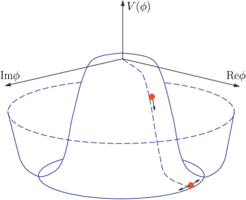
Figure 1: The scalar potential. Bullets show the evolution of the scalar field. Arrows at the end point at the bottom of the potential indicate that there are perturbations of the phase.

The scenario proceeds with the assumption that the scalar potential $V(\phi)$ has, in fact, a minimum at some large value of $|\phi|$, and that the modulus of the field $\phi$ eventually gets relaxed to the minimum, see figure 1. The simplest option concerning further evolution of the perturbations $\delta\theta$ is that they are superhorizon in the conventional sense by the time the conformal rolling stage ends. We proceed under this assumption. The phase perturbations remain frozen out, and their power spectrum remains flat. At some much later cosmological epoch, the perturbations of the phase are converted into the adiabatic scalar perturbations by, e.g., the curvaton mechanism [14] (in that case $\theta$ is a pseudo-Nambu-Goldstone curvaton, and reprocessing occurs as discussed in ref. [15]) or modulated decay mechanism [16, 17]. In either case, the power spectrum is not distorted, so the resulting adiabatic perturbations have flat primordial power spectrum. If conformal invariance is not exact at the rolling stage, the scalar power spectrum has small tilt, which depends on both the strength of the violation of conformal invariance and the evolution of the scale factor at the rolling stage [18].

A peculiar property of the model is that the modulus of the rolling field also acquires perturbations. At late times, modes of the modulus (i.e., radial direction) have red power spectrum (see section 2.2 for details),

$$\sqrt{{\cal P}_{|\phi|}(k)}\propto k^{-1}\;.$$ (4)

One consequence is that there are perturbations of the energy density with red spectrum right after the conformal rolling stage, but before the modulus freezes out at the minimum of $V(\phi)$. These are not dangerous, provided that the energy density of the field $\phi$ is small compared to the total energy density at all times before the modulus freezes out, i.e., the cosmological evolution is governed by some other matter at that early epoch. In this paper we assume that this is indeed the case.

The second consequence is that the infrared radial modes interact with the perturbations of the phase, and in principle may have strong effect on the latter. This is one of the issues we address in this paper. We show that to the linear order in $h$, the infrared effects can be absorbed into field redefinition, so there is no gross modification of the results of the linear analysis due to the effect of the infrared modes.

The large wavelength modes of $\delta|\phi|$ are not entirely negligible, however. The modes whose present wavelengths exceed the present Hubble size $H_{0}^{-1}$ induce statistical anisotropy in the perturbations of the phase $\delta\theta$, and hence in the resulting adiabatic perturbations: the power spectrum of the adiabatic perturbation $\zeta$ has the following form,

$${\cal P}_{\zeta}({\bf k})={\cal P}_{0}(k)\left(1+c_{1}\cdot h\cdot\frac{H_{0}}{k}\cdot\hat{k}_{i}\hat{k}_{j}w_{ij}-c_{2}\cdot h^{2}\cdot({\bf\hat{k}u})^{2}\right)\;.$$ (5)

The first non-trivial term, linear in $h$, is free of the infrared effects; $w_{ij}$ is a traceless symmetric tensor of a general form with unit normalization, $w_{ij}w_{ij}=1$, ${\bf\hat{k}}$ is a unit vector, ${\bf\hat{k}}={\bf k}/k$, and $c_{1}$ is a constant of order 1 whose actual value is undetermined because of the cosmic variance. In the last term, ${\bf u}$ is some unit vector independent of $w_{ij}$, and the positive parameter $c_{2}$ is logarithmically enhanced due to the infrared effects. This is the first place where the deep infrared modes show up. Clearly, their effect is subdominant for small $h$.

The statistical anisotropy encoded in the last term in (5) is similar to that commonly discussed in inflationary context [19], and, indeed, generated in some concrete inflationary models [20]: it does not decay as momentum increases and has special tensorial form $({\bf\hat{k}u})^{2}$ with constant ${\bf u}$. On the other hand, the first non-trivial term in (5) has the general tensorial structure and decreases with momentum. The latter property is somewhat similar to the situation that occurs in cosmological models with the anisotropic expansion before inflation [21]. Overall, the statistical anisotropy (5) may be quite substantial, since there are no strong bounds on $h$ at least for the modulated decay mechanism of conversion of the phase perturbations into adiabatic ones.

The non-linearity of the scalar potential gives rise to the non-Gaussianity of the perturbations of the phase $\delta\theta$, and hence the adiabatic perturbations in our scenario, over and beyond the non-Gaussianity that may be generated at the time when the phase perturbations get reprocessed into the adiabatic perturbations. In view of the result outlined above, this non-Gaussianity is not plagued by the infrared effects at the first non-trivial order in $h$. Therefore, the gradient expansion of the effective background is useless for the study of the non-Gaussianity, and we have to perform a hard-core calculation. Because of the symmetry $\theta\to-\theta$, the bispectrum of the phase vanishes, while the general expression for the trispectrum is rather cumbersome. It simplifies in the folded limit (according to the nomenclature of ref. [22]); the explicit form of the trispectrum in this limit is given by eq. (45).

The paper is organized as follows. In section 2 we review the linear analysis of the model. In section 3 we study the effect of infrared modes of the modulus $\delta|\phi|$ on the perturbations of the phase $\delta\theta$ at the leading and subleading orders of the gradient expansion, and to the linear order in $h$. Statistical anisotropy is analysed in section 4. Non-Gaussianity is considered in section 5. We conclude in section 6.

2 Linear analysis

At the conformal rolling stage, the dynamics of the scalar field is governed by the action

$$S[\phi]=\int d^{4}x\sqrt{-g}\left[g^{\mu\nu}\partial_{\mu}\phi^{*}\partial_{\nu}\phi+\frac{R}{6}\phi^{*}\phi-V(\phi)\right]\;.$$

where the scalar potential $V(\phi)$ is negative and has conformally invariant form (1). In terms of the field $\chi=a\phi$, the field equation is

$$\eta^{\mu\nu}\partial_{\mu}\partial_{\nu}\chi-2h^{2}|\chi|^{2}\chi=0\;.$$ (6)

Spatially homogeneous background approaches the late-time attractor (2).

2.1 Perturbations of phase

At the linearized level, the perturbations of the phase and modulus of the field $\phi$ decouple from each other. Let us begin with the perturbations of the phase, or, for real background (2), perturbations of the imaginary part $\chi_{2}\equiv\mbox{Im}~{}\chi/\sqrt{2}$. They obey the linearized equation,

$$(\delta\chi_{2})^{\prime\prime}-\partial_{i}\partial_{i}\;\delta\chi_{2}-2h^{2}\chi_{c}^{2}\;\delta\chi_{2}=0\;,$$ (7)

where prime denotes the derivative with respect to $\eta$. Let ${\bf k}$ be conformal momentum of perturbation. An important assumption of the entire scenario is that the rolling stage begins early enough, so that there is time at which

$$k(\eta_{*}-\eta)\gg 1\;.$$ (8)

Since the momenta $k$ of cosmological significance are as small as the present Hubble parameter, this inequality means that the duration of the rolling stage in conformal time is longer than the conformal time elapsed from, say, the beginning of the hot Big Bang expansion to the present epoch. This is only possible if the hot Big Bang stage was preceded by some other epoch, at which the standard horizon problem is solved; the mechanism we discuss in this paper is meant to operate at that epoch. We note in passing that the latter property is inherent in most, if not all, mechanisms of the generation of cosmological perturbations.

Equation (7) is exactly the same as equation for minimally coupled massless scalar field in the de Sitter background. For future reference, we write its solution in the following form:

$$\delta\chi_{2}({\bf x},\eta)=\int~{}\frac{d^{3}k}{(2\pi)^{3/2}\sqrt{2k}}~{}\left(\delta\chi_{2}^{(-)}({\bf k},{\bf x},\eta)\hat{A}_{\bf k}+h.c.\right)\;.$$

Here

$$\delta\chi_{2}^{(-)}({\bf k},{\bf x},\eta)=\mbox{e}^{i{\bf kx}-ik\eta_{*}}\cdot F(k,\eta_{*}-\eta)\;,$$ (9)

with

$$F(k,\xi)=-\sqrt{\frac{\pi}{2}k\xi}~{}H^{(1)}_{3/2}(k\xi)$$ (10)

and $H^{(1)}_{3/2}$ is the Hankel function. At early times, the mode oscillates,

$$\delta\chi_{2}^{(-)}({\bf k},{\bf x},\eta)=\mbox{e}^{i{\bf kx}-ik\eta}\;.$$ (11)

so $\hat{A}_{\bf k}$ and $\hat{A}_{\bf k}^{\dagger}$ are annihilation and creation operators obeying the standard commutational relation, $[\hat{A}_{\bf k},\hat{A}_{\bf k^{\prime}}^{\dagger}]=\delta({\bf k}-{\bf k^{\prime}})$. As usual, we assume that the field $\delta\chi_{2}$ is initially in its vacuum state.

At late times, when $k(\eta_{*}-\eta)\ll 1$, the perturbations of the phase are time-independent,

$$\delta\theta({\bf x})=\frac{\delta\chi_{2}({\bf x},\eta)}{\chi_{c}(\eta)}=ih\int~{}\frac{d^{3}k}{4\pi^{3/2}k^{3/2}}~{}\mbox{e}^{i{\bf kx}-ik\eta_{*}}\hat{A}_{\bf k}+h.c.$$ (12)

This expression describes Gaussian random field (cf. ref. [23]) whose power spectrum is given by (3).

The phase perturbations can be converted into adiabatic ones by at least two mechanisms. One operates if $\theta$ is actually pseudo-Nambu–Goldstone field that lands at a slope of its potential. This mechanism produces the non-Gaussianity of local form in the adiabatic perturbations. For generic values of the phase at landing, $\theta_{c}\sim\pi/2$, non-observation of the non-Gaussianity [1] implies ${\cal P}_{\delta\theta}\lesssim 10^{-4}$, cf. ref. [15], so that the correct scalar amplitude is obtained for

$$h\lesssim 10^{-2}\;.$$ (13)

Generally speaking, such a constraint is not characteristic of the alternative, modulated decay mechanism [16, 17]. In that case, if the relevant mass or width depends linearly on $\theta$, the resuling non-Gaussianity parameter is fairly small (see refs. [17, 24] for details), $f_{NL}\sim 1$, in comfortable agreement with the existing limit [1].

2.2 Perturbations of modulus

Let us now consider the radial perturbations or, with our convention of real background $\chi_{c}$, perturbations of the real part $\chi_{1}\equiv\mbox{Re}~{}\chi/\sqrt{2}$. At the linearized level, they obey the following equation at conformal rolling stage,

$$(\delta\chi_{1})^{\prime\prime}-\partial_{i}\partial_{i}~{}\delta\chi_{1}-6h^{2}\chi_{c}^{2}\delta\chi_{1}\equiv(\delta\chi_{1})^{\prime\prime}-\partial_{i}\partial_{i}~{}\delta\chi_{1}-\frac{6}{(\eta_{*}-\eta)^{2}}\delta\chi_{1}=0\;.$$

Its solution that tends to properly normalized mode as $k(\eta_{*}-\eta)\to\infty$ is

$$\delta\chi_{1}=-\mbox{e}^{i{\bf kx}-ik\eta_{*}}\cdot\frac{i}{4\pi}\sqrt{\frac{\eta_{*}-\eta}{2}}H_{5/2}^{(1)}\left[k(\eta_{*}-\eta)\right]\cdot\hat{B}_{\bf k}+h.c.\;,$$

where $\hat{B}_{\bf k}$, $\hat{B}_{\bf k}^{\dagger}$ is another set of annihilation and creation operators. At late times, when $k(\eta_{*}-\eta)\ll 1$ one has

$$\delta\chi_{1}=-\mbox{e}^{i{\bf kx}-ik\eta_{*}}\cdot\frac{3}{4\pi^{3/2}}\frac{1}{k^{5/2}(\eta_{*}-\eta)^{2}}\cdot\hat{B}_{\bf k}+h.c.\;.$$

Hence, the resulting perturbations of the modulus have red power spectrum (4).

The dependnce $\delta\chi_{1}\propto(\eta_{*}-\eta)^{-2}$ is naturally interpreted in terms of the local shift of the “end time” parameter $\eta_{*}$. Indeed, with the background field given by (2), the sum $\chi_{c}+\delta\chi_{1}/\sqrt{2}$, i.e., the radial field including perturbations, is the linearized form of

$$\chi_{c}[\eta_{*}({\bf x})-\eta]=\frac{1}{h[\eta_{*}({\bf x})-\eta]}\;,$$ (14)

where

$$\eta_{*}({\bf x})=\eta_{*}+\delta\eta_{*}({\bf x})$$ (15)

and

$$\delta\eta_{*}({\bf x})=\frac{3h}{4\sqrt{2}\pi^{3/2}}\int~{}\frac{d^{3}k}{k^{5/2}}\left(\mbox{e}^{i{\bf kx}-ik\eta_{*}}\cdot\hat{B}_{\bf k}+h.c.\right)\;.$$ (16)

So, the infrared radial modes modify the effective background by transforming the “end time” parameter $\eta_{*}$ into random field that slowly varies in space, as given in eqs. (14), (15).

It is worth noting that the infrared modes contribute both to the field $\delta\eta_{*}({\bf x})$ itself and to its spatial derivative. The contribution of the modes which are superhorizon today, i.e., have momenta $k\lesssim H_{0}$, to the variance of the latter is given by

$$\langle\partial_{i}\eta_{*}({\bf x})\partial_{j}\eta_{*}({\bf x})\rangle_{k\lesssim H_{0}}=\delta_{ij}\cdot\frac{3h^{2}}{8\pi}\int_{k\lesssim H_{0}}\frac{dk}{k}=\delta_{ij}\cdot\frac{3h^{2}}{8\pi}\log\frac{H_{0}}{\Lambda}\;,$$ (17)

where $\Lambda$ is the infrared cutoff which parametrizes our ignorance of the dynamics at the beginning of the conformal rolling stage.

3 Effect of infrared radial modes on perturbations of phase: first order in $h$

Let us see how the interaction with the infrared radial modes affects the properties of the perturbations of the phase $\delta\theta$. To this end, we consider perturbations of the imaginary part $\delta\chi_{2}$, whose wavelengths are much smaller than the scale of the spatial variation of the modulus (see ref. [25] for details). Because of the separation of scales, perturbations $\delta\chi_{2}$ can still be treated in the linear approximation, but now in the background (14).

Since our concern is the infrared part of $\eta_{*}({\bf x})$, we make use of the spatial gradient expansion, consider, for the time being, a region near the origin and write

$$\eta_{*}({\bf x})=\eta_{*}(0)-v_{i}x_{i}+\dots\;,$$ (18)

where

$$v_{i}=-\partial_{i}\eta_{*}({\bf x})|_{{\bf x}=0}\;,$$

and dots denote higher order terms in ${\bf x}$. Importantly, the field $\partial_{i}\partial_{j}\eta_{*}({\bf x})$ has blue power spectrum, so the major effect of the infrared modes is accounted for by considering the two terms written explicitly in (18). In this section we work at this, first order of the gradient expansion. Furthermore, we assume in what follows that

$$|{\bf v}|\ll 1\;,$$ (19)

and in this section we neglect corrections of order ${\bf v}^{2}$. The expansion in $|{\bf v}|$ is legitimate, since the field ${\bf v}({\bf x})$ has flat power spectrum, so the expansion in $|{\bf v}|$ is the expansion in $h$, modulo infrared logarithms. We postpone to section 4.2 the analysis of the leading effect that occurs at the order ${\bf v}^{2}$.

Keeping the two terms in (18) only, we have, instead of eq. (2),

$$\chi_{c}=\frac{1}{h[\eta_{*}(0)-\eta-{\bf vx}]}\;.$$ (20)

This expression involves the combination $\eta_{*}(0)-(\eta+{\bf vx})$. We interpret it as the local time shift and Lorentz boost of the original background (2). Note that the field (20) is a solution to the field equation (6) in our approximation. Our interpretation enables us to find the solutions to eq. (7) with the background (20) and initial condition (11): these are obtained by time translation and Lorentz boost of the original solution (9), (10):

$$\delta\chi_{2}^{(-)}({\bf k},{\bf x},\eta)=\mbox{e}^{i{\bf q}({\bf x}+{\bf v}\eta)-iq\eta_{*}(0)}\cdot F(q,\eta_{*}(0)-\eta-{\bf vx})\;,$$ (21)

where the function $F$ is still defined by (10), the Lorentz-boosted momentum is

$${\bf q}={\bf k}+k{\bf v}\;,\;\;\;\;q=|{\bf q}|=k+{\bf kv}\;,$$ (22)

and it is understood that terms of order ${\bf v}^{2}$ must be neglected. We consider corrections of order $\partial_{i}\partial_{j}\eta_{*}({\bf x})$ and ${\bf v^{2}}$ to this solution in sections 4.1 and 4.2, respectively.

We find from eqs. (20) and (21) that the perturbations of the phase again freeze out as $k[\eta_{*}({\bf x})-\eta]\to 0$, now at

$$\delta\theta({\bf x})=\frac{\delta\chi_{2}({\bf x})}{\chi_{c}(\bf x)}=i\int~{}\frac{d^{3}k}{\sqrt{k}}\frac{h}{4\pi^{3/2}q}~{}\mbox{e}^{i{\bf kx}-ik\eta_{*}({\bf x})}\hat{A}_{\bf k}+h.c.\;,$$ (23)

This result implies that to the first order of the gradient expansion we limit ourselves in this section, the properties of the random field $\delta\theta$ are the same as those of the linear field (12). Indeed, since $\eta_{*}({\bf x})=\eta_{*}(0)-{\bf vx}$ in (23), the infrared effects are removed by the field redefinition,

$$\hat{\mathcal{A}}_{\bf q}=\mbox{e}^{-ik\eta_{*}(0)}\sqrt{\frac{k}{q}}\hat{A}_{\bf k}\;,$$ (24)

where ${\bf k}$ and ${\bf q}$ are still related by (22). Due to the Lorentz-invariance of the measure $d^{3}k/k$, the operators $\hat{\mathcal{A}}_{\bf q}$, $\hat{\mathcal{A}}_{\bf q}^{\dagger}$ obey the standard commutational relations, while in our approximation, the field (23), written in terms of these operators, coincides with the linear field (12). We conclude that the infrared radial modes are, in fact, not particularly dangerous, as they do not grossly affect the properties of the field $\delta\theta$.

4 Statistical anisotropy

4.1 First order in $h$

To the first order in $h$, the non-trivial effect of the large wavelength perturbations $\delta\eta_{*}({\bf x})$ on the perturbations of the phase occurs for the first time at the second order in the gradient expansion, i.e., at the order $\partial_{i}\partial_{j}\eta_{*}$. Let us concentrate on the effect of the modes of $\delta\eta_{*}$ whose present wavelengths exceed the present Hubble size. We are dealing with one realization of the random field $\delta\eta_{*}$, hence at the second order of the gradient expansion, $\partial_{i}\partial_{j}\eta_{*}$ is merely a tensor, constant throughout the visible Universe. In this section we calculate the statistical anisotropy associated with this tensor.

To this end, we make use of the perturbation theory in $\partial_{i}\partial_{j}\eta_{*}$. The background (14) is no longer the solution to the field equation (6) at the second order in the gradient expansion. The relevant combination entering eq. (7) for the perturbations of the imaginary part is now given by (see ref. [25] for details)

$$2h^{2}\chi_{c}^{2}=\frac{2}{(\eta_{*}({\bf x})-\eta)^{2}}+\frac{2}{3}\frac{\partial_{i}\partial_{i}\eta_{*}}{\eta_{*}-\eta}\;.$$ (25)

The solution to eq. (7) with background (25) and initial condition (11) in the late-time regime is

$$\delta\chi_{2}^{(-)}({\bf k},{\bf x},\eta)=\frac{i\mbox{e}^{i{\bf k}{\bf x}-ik\eta_{*}({\bf x})}}{q(\eta_{*}-\eta)}\left(1-\frac{\pi}{2k}\cdot\frac{k_{i}k_{j}}{k^{2}}\partial_{i}\partial_{j}\eta_{*}+\frac{\pi}{6k}\partial_{i}\partial_{i}\eta_{*}\right)\;.$$

The two non-trivial terms in parenthesis give the correction to the power spectrum of the phase perturbations due to the radial modes whose whavelengths exceed the present Hubble size. The same correction is characteristic of the adiabatic perturbations, so we have finally

$${\cal P}_{\zeta}=A_{\zeta}\left[1-\frac{\pi}{k}\cdot\frac{k_{i}k_{j}}{k^{2}}\left(\partial_{i}\partial_{j}\eta_{*}-\frac{1}{3}\delta_{ij}\partial_{k}\partial_{k}\eta_{*}\right)\right]\;.$$ (26)

Notably, the angular average of the correction vanishes, so we are dealing with the statistical anisotropy proper.

Neither the magnitude nor the exact form of the tensor $\partial_{i}\partial_{j}\eta_{*}-(1/3)\delta_{ij}\partial_{k}\partial_{k}\eta_{*}$ can be unambiguously predicted because of the cosmic variance. To estimate the strength of the statistical anisotropy, let us consider the variance

$$\left\langle\left(\partial_{i}\partial_{j}\eta_{*}-\frac{1}{3}\delta_{ij}\partial_{k}\partial_{k}\eta_{*}\right)\cdot\left(\partial_{i}\partial_{j}\eta_{*}-\frac{1}{3}\delta_{ij}\partial_{k}\partial_{k}\eta_{*}\right)\right\rangle_{k\lesssim H_{0}}\simeq\frac{3h^{2}}{8\pi^{2}}H_{0}^{2}\;,$$

where the notation reflects the fact that we take into account only those modes whose present wavelengths exceed the present Hubble size. In this way we arrive at the first non-trivial term in (5). Higher orders in the gradient expansion give contributions to the statistical anisotropy which are suppressed by extra factors of $H_{0}/k$.

4.2 Order $h^{2}$: contribution of deep infrared modes

Let us now turn to the statistical anisotropy at the second order in $h$. Since the overall time shift $\eta_{*}(0)$ is irrelevant, the major contribution at this order is proportional to the log-enhanced combination $\partial_{i}\eta_{*}\partial_{j}\eta_{*}\equiv v_{i}v_{j}$. Hence, we use the two terms of the derivative expansion, explicitly written in (18).

To order ${\bf v}^{2}$, the function (20) is no longer a solution to the field equation (6). Instead, the solution is

$$\chi_{c}=\frac{1}{h\gamma\left[\eta_{*}(0)-\eta-{\bf vx}\right]}\;.$$ (27)

So, it is appropriate to study the solutions to eq. (7) in this background. It is straightforward to see that the solution that obeys the initial condition (11) is

$$\delta\chi_{2}^{(-)}({\bf k},{\bf x},\eta)=\mbox{e}^{iq_{||}\gamma(x_{||}+v\eta)+i{\bf q}^{T}{\bf x}^{T}-iq\gamma\eta_{*}(0)}\cdot F\left[q,\gamma(\eta_{*}(0)-\eta-{\bf vx})\right]\;,$$ (28)

where the Lorentz-boosted momentum is, as usual, $q_{||}=\gamma(k_{||}+kv)$, ${\bf q}^{T}={\bf k}^{T}$, $q=\gamma(k+k_{||}v)$, $\gamma=(1-v^{2})^{-1/2}$, and notations $||$ and $T$ refer to components parallel and normal to ${\bf v}$, respectively.

According to the scenario discussed in this paper, the phase perturbations $\delta\theta$ freeze out at the hypersurface $\eta=\eta_{*}(0)-{\bf vx}\equiv\eta_{*}(0)-vx_{||}$ and then stay constant in the cosmic time $\eta$. It follows from (27) and (28) that at late times, the perturbations of the phase are

$$\delta\theta({\bf x})=\int~{}\frac{d^{3}q}{\sqrt{q}}\frac{h}{4\pi^{3/2}q}~{}\mbox{e}^{i\gamma^{-1}q_{||}x_{||}+i{\bf q}^{T}{\bf x}^{T}}\hat{{\mathcal{A}}}_{\bf q}+h.c.\;,$$ (29)

where the operators $\hat{{\mathcal{A}}}_{\bf q}$ are defined by (24) and obey the standard commutational relations, and we have omitted irrelevant constant phase factor. We see that to the order ${\bf v}^{2}$, the effect of the deep infrared modes is encoded in the factor $\gamma^{-1}$ in the first term in the exponent: the momentum of perturbation labeled by ${\bf q}$ is actually equal to ${\bf p}=(\gamma^{-1}q_{||},{\bf q}^{T})\;.$ Accordingly, the power spectrum (omitting the correction discussed in section 4.1) is given by

$$\mathcal{P}_{\zeta}({\bf k})=A_{\zeta}\frac{k^{3}}{[(\gamma k_{||})^{2}+({\bf k}^{T})^{2}]^{3/2}}=A_{\zeta}\left(1-\frac{3}{2}\frac{({\bf kv})^{2}}{k^{2}}\right)\;.$$

Hence, we have arrived at the last term in (5). Again, neither the direction of ${\bf v}$ nor its length can be unambiguously calculated because of cosmic variance; recall, however, that the value of $|{\bf v}|$, and hence the parameter $c_{2}$ in (5), is logarithmically enhanced due to the infrared effects, see (17).

In the case of the curvaton mechanism of conversion of the phase perturbations into the adiabatic ones, both terms in the statistical ansotropy (5) are small because of the bound (13). On the other hand, the effect may be stronger in the case of the modulated decay mechanism.

5 Non-Gaussianity

In this section we discuss non-Gaussianity of the phase perturbations (see ref. [26] for details). Due to the symmetry $\theta\to-\theta$, the bispectrum $\langle\delta\theta\delta\theta\delta\theta\rangle$ as well as odd higher order correlators vanish identically and we have to deal with the trispectrum. Since the infrared modes are irrelevant to the leading order in $h$, the gradient expansion of the modulus is useless, and we make use of the conventional perturbation theory. It is convenient to perform the calculation in terms of the perturbations of the modulus and phase,

$$\chi=\left(\chi_{c}+\frac{\delta\rho}{\sqrt{2}}\right)\exp\left(i\frac{\delta\theta}{\sqrt{2}}\right)\;,$$

and employ the IN-IN formalism (see, e.g., ref.[27]). The late-time expectation value of an operator $\mathcal{O}$ is given by

$$\langle\mathcal{O}\rangle=\left\langle\left[\overline{T}\exp\left(i\int\limits_{-\infty}^{0}dx_{0}d^{3}x\mathcal{H}_{I}\right)\right]\mathcal{O}_{(I)}\left[T\exp\left(-i\int\limits_{-\infty}^{0}dx_{0}d^{3}x\mathcal{H}_{I}\right)\right]\right\rangle$$ (30)

where the time variable is $x^{0}=\eta-\eta_{*}$ (note that $x^{0}<0$), $\bar{T}$ and $T$ denote anti-time ordering and time ordering, respectively, and $\mathcal{H}_{I}$ and $\mathcal{O}_{(I)}$ are the interaction part of the Hamiltonian and operator $\mathcal{O}$ in the interaction picture. In what follows we are interested in the first nontrivial order in $h$, so the relevant part of $\mathcal{H}_{I}$ is

$$\mathcal{H}_{I}=\frac{\chi_{c}\delta\rho}{\sqrt{2}}\left((\partial_{i}\delta\theta)^{2}-(\delta\theta^{\prime})^{2}\right)\;.$$ (31)

Upon substituting (31) into (30) one finds the following expression for the connected part of the four-point function

$$\langle\delta\theta_{\mathbf{x}}\delta\theta_{\mathbf{y}}\delta\theta_{\mathbf{z}} \delta\theta_{\mathbf{w}}\rangle=\frac{8}{h^{4}}\int\limits_{-\infty}^{0}dx_{0}^{\prime}dx_{0}^{\prime\prime}d^{3}x^{\prime}d^{3}x^{\prime\prime}\chi_{c}(x_{0}^{\prime})\chi_{c}(x_{0}^{\prime\prime})\left[Q_{x^{\prime}\mathbf{xy}}Q_{x^{\prime\prime}\mathbf{zw}}\mathrm{Re}D_{\rho}(x^{\prime},x^{\prime\prime})-\right.$$ (32)

$$-\left.\mathrm{Im}D_{\rho}(x^{\prime},x^{\prime\prime})\left\{\Theta(x_{0}^{\prime}-x_{0}^{\prime\prime})Q_{x^{\prime}\mathbf{xy}}R_{x^{\prime\prime}\mathbf{zw}}-\Theta(x_{0}^{\prime\prime}-x_{0}^{\prime})R_{x^{\prime}\mathbf{xy}}Q_{x^{\prime\prime}\mathbf{zw}}\right\}\right]+$$

$$\qquad\qquad\qquad\qquad+[y\leftrightarrow z]+[y\leftrightarrow w]$$

where

$$R_{x^{\prime}\mathbf{xy}} = \mathrm{Re}\left[\frac{\partial}{\partial x^{\prime}_{\mu}}D(x^{\prime},\mathbf{x},x^{0}=0)\frac{\partial}{\partial{x^{\prime}}^{\mu}}D(x^{\prime},\mathbf{y},y^{0}=0)\right]$$

$$Q_{x^{\prime}\mathbf{xy}} = \mathrm{Im}\left[\frac{\partial}{\partial x^{\prime}_{\mu}}D(x^{\prime},\mathbf{x},x^{0}=0)\frac{\partial}{\partial{x^{\prime}}^{\mu}}D(x^{\prime},\mathbf{y},y^{0}=0)\right]\;,$$ (33)

$D(x,y)$ and $D_{\rho}(x,y)$ are the pairings of $\delta\theta$ and $\delta\rho$, respectively, $D(x,y)=\langle\delta\theta(x)\delta\theta(y)\rangle$, etc. Recalling that in the interaction picture $\delta\theta$ and $\delta\rho$ coincide with $\delta\chi_{2}/\chi_{c}$ and $\delta\chi_{1}$, respectively, and using the results of sec. 2 one gets

$$D(x^{\prime},\mathbf{x},x_{0}=0)=\frac{ih^{2}}{32\pi^{2}}\sqrt{\frac{2}{\pi}}\int\limits\frac{d^{3}k}{k^{3}}(-kx_{0}^{\prime})^{3/2}H_{3/2}^{(1)}(-kx_{0}^{\prime})\mathrm{e}^{i\mathbf{k}(\mathbf{x^{\prime}-x})}$$ (34)

$$D_{\rho}(x,y)=\frac{1}{32\pi^{2}}\int\limits d^{3}k\sqrt{x_{0}y_{0}}H_{5/2}^{(1)}(-kx_{0})H_{5/2}^{(2)}(-ky_{0})\mathrm{e}^{i\mathbf{k}(\mathbf{x}-\mathbf{y})}\;.$$ (35)

It is worth noting that in the derivation of eq. (32) we used the following property of the pairings

$$D(x,y)=D^{*}(y,x)\;,\ \ \ \ D_{\rho}(x,y)=D_{\rho}^{*}(y,x)\;.$$

To find the explicit form of the functions $R_{x^{\prime}\mathbf{xy}}$ and $Q_{x^{\prime}\mathbf{xy}}$ we substitute (34) into (33). Using the explicit form of the Hankel function, we get

$$R_{x^{\prime}\mathbf{xy}} = -\frac{h^{4}}{8(2\pi)^{6}}\int\limits\frac{d^{3}k_{1}d^{3}k_{2}}{k_{1}^{3}k_{2}^{3}}\mathrm{e}^{i\left[(\mathbf{k}_{1}+\mathbf{k}_{2})\mathbf{x^{\prime}}-\mathbf{k}_{1}\mathbf{x}-\mathbf{k}_{2}\mathbf{y}\right]}\tilde{R}(k_{1},k_{2},q,-x_{0}^{\prime})$$

$$Q_{x^{\prime}\mathbf{xy}} = -\frac{h^{4}}{8(2\pi)^{6}}\int\limits\frac{d^{3}k_{1}d^{3}k_{2}}{k_{1}^{3}k_{2}^{3}}\mathrm{e}^{i\left[(\mathbf{k}_{1}+\mathbf{k}_{2})\mathbf{x^{\prime}}-\mathbf{k}_{1}\mathbf{x}-\mathbf{k}_{2}\mathbf{y}\right]}\tilde{Q}(k_{1},k_{2},q,-x_{0}^{\prime})$$ (36)

where

$$\tilde{R}(k_{1},k_{2},q,\xi) = \cos(\xi(k_{1}+k_{2}))\cdot\left[\xi^{2}k_{1}k_{2}(q^{2}-(k_{1}+k_{2})^{2})+k_{1}^{2}+k_{2}^{2}-q^{2}\right]+$$

$$+\sin(\xi(k_{1}+k_{2}))\cdot\xi(k_{1}+k_{2})(k_{1}^{2}+k_{2}^{2}-q^{2})$$

$$\tilde{Q}(k_{1},k_{2},q,\xi) = \sin(\xi(k_{1}+k_{2}))\cdot\left[\xi^{2}k_{1}k_{2}(q^{2}-(k_{1}+k_{2})^{2})+k_{1}^{2}+k_{2}^{2}-q^{2}\right]-$$ (37)

$$-\cos(\xi(k_{1}+k_{2}))\cdot\xi(k_{1}+k_{2})(k_{1}^{2}+k_{2}^{2}-q^{2}),$$

and

$$\mathbf{q=k}_{1}+\mathbf{k}_{2}.$$

The formula (32), converted to momentum representation, gives the general expression for the trispectrum of the phase.

Let us now consider the folded configuration, namely, the trispectrum in momentum representation

$$G^{(4)}(\mathbf{Q,P,q})=\left\langle\delta\theta\left(\frac{\mathbf{q}}{2}+\mathbf{Q}\right)\delta\theta\left(\frac{\mathbf{q}}{2}-\mathbf{Q}\right)\delta\theta\left(-\frac{\mathbf{q}}{2}+\mathbf{P}\right)\delta\theta\left(-\frac{\mathbf{q}}{2}-\mathbf{P}\right)\right\rangle$$ (38)

with

$$Q\sim P\gg q\;.$$ (39)

In real space, this limit corresponds to the following configuration

$$|\mathbf{x-y}|\sim|\mathbf{z-w}|\ll|\mathbf{x-z}|\sim|\mathbf{y-w}|\;,$$

i.e., the four points $\mathbf{x,y,z,w}$ form, crudely speaking, an elongated parallelogram with the short edge $\varepsilon\sim|\mathbf{x-y}|$ and the long edge $L\sim|\mathbf{x-z}|$.

To proceed, we consider in the small $q$ limit the contribution to $G^{(4)}$ coming from the first term in the square brackets in (32). Making use of eqs. (35), (36) and (37), we find

$$G^{(4)}(\mathbf{Q,P,q})=\frac{h^{2}\pi}{32}\frac{1}{k_{+}^{3}k_{-}^{3}p_{+}^{3}p_{-}^{3}}\times$$ (40)

$$\phantom{\times}\times\!\!\int\limits_{0}^{\infty}\!\!\frac{d\xi d\chi}{\sqrt{\xi\chi}}\tilde{Q}(k_{+},k_{-},q,\xi)\tilde{Q}(p_{+},p_{-},q,\chi)\left[Y_{5/2}(q\xi)Y_{5/2}(q\chi)+J_{5/2}(q\xi)J_{5/2}(q\chi)\right],$$

where

$$\mathbf{k}_{\pm}=\mathbf{q/2\pm Q}\;,\ \ \ \mathbf{p}_{\pm}=\mathbf{-q/2\pm Q}\;,$$ (41)

and $J_{5/2}$, $Y_{5/2}$ are the Bessel functions of the first and the second kind, respectively. We see that the integral over $\xi$ and $\chi$ splits into a sum of products of two integrals

$$\mathcal{J}(k_{+},k_{-},q) = \int\limits_{0}^{\infty}\frac{d\xi}{\sqrt{\xi}}\tilde{Q}(k_{+},k_{-},q,\xi)J_{5/2}(q\xi)$$ (42)

$$\mathcal{Y}(k_{+},k_{-},q) = \int\limits_{0}^{\infty}\frac{d\xi}{\sqrt{\xi}}\tilde{Q}(k_{+},k_{-},q,\xi)Y_{5/2}(q\xi)\;.$$ (43)

These integrals converge in both the lower and upper limits. This means, in particular, that in the small $q$ limit (if one considers $k_{\pm}$ and $q$ as independent variables) the leading behaviour of the integrals is

$$\mathcal{J}(q)\propto q^{5/2}\;,\ \ \ \mathcal{Y}(q)\propto q^{-5/2}\;.$$

Thus, we can neglet $\mathcal{J}$. The direct evoluation of the integral (43) gives

$$\mathcal{Y}(k_{+},k_{-},q) = -\frac{1}{2}\sqrt{\frac{\pi}{2}}\frac{1}{q^{5/2}}\left[3(k_{+}^{2}-k_{-}^{2})^{2}-2(k_{+}^{2}+k_{-}^{2})q^{2}-q^{4}\right]=$$ (44)

$$=\sqrt{\frac{2\pi}{q}}Q^{2}\left[1-3\left(\frac{\mathbf{qQ}}{qQ}\right)^{2}+O(q^{2}/Q^{2})\right]$$

where in the second line we make use of (41). We see that the contributions proportional to $q^{-5}$ and $q^{-3}$ vanish, as should be the case in view of the results of section 3.

Upon substituting eq. (44) into eq. (40) we finally get in the small $q$ limit the contribution to $G^{(4)}$ coming from the first term in the square brackets of (32):

$$G^{(4)}(\mathbf{Q},\mathbf{P},\mathbf{q})=\frac{h^{2}\pi^{2}}{16}\frac{1}{qQ^{4}P^{4}}\left[1-3\left(\frac{\mathbf{qQ}}{qQ}\right)^{2}\right]\left[1-3\left(\frac{\mathbf{qP}}{qP}\right)^{2}\right]+O(q/Q)\;.$$ (45)

This is actually the final expression for the trispectrum in the folded limit. To see this we, first note that $q$ is the momentum carried by the pairing $D_{\rho}$ in (32), i.e. the regime (39) corresponds to the infrared effects associated with the perturbations of the modulus. It follows from (35) that at small momenta the leading behaviour of $D_{\rho}$ is

$$\mathrm{Re}D_{\rho}\sim{q^{-5}}\,,\ \ \ \ \mathrm{Im}D_{\rho}\sim q^{0}\;.$$

Hence, only the first term in the square brackets in eq. (32) contributes to $G^{(4)}$: the time integral of the second term as well as the second term itself are regular as $q\to 0$. The crossing term (last line in (32)) does not contribute to (45) as well. The reason is that the momentum carried by $D_{\rho}$ in that case is $2(\mathbf{Q+P})$ rather then $\mathbf{q}$, so it is large.

6 Conclusion

We conclude by making a few remarks.

First, our mechanism of the generation of the adiabatic perturbations can work in any cosmological scenario that solves the horizon problem of the hot Big Bang theory, including inflation, bouncing/cyclic scenario, pre-Big Bang, etc. In some of these scenarios (e.g., bouncing Universe), the assumption that the phase perturbations are superhorizon in conventional sense by the end of the conformal rolling stage may be non-trivial. It would be of interest to study also the opposite case, in which the phase evolves for some time after the end of conformal rolling.

Second, we concentrated in the first part of this paper on the effect of infrared radial modes, and employed the derivative expansion. The expressions like (23), which we obtained in this way, must be used with caution, however. Bold usage of (23) would yield, e.g., non-vanishing equal-time commutator $[\theta({\bf x}),\theta({\bf y})]$, which would obviously be a wrong result. The point is that the formula (23) is valid in the approximation ${\bf v}=\mbox{const}$; with this understanding, the equal-time commutator vanishes, as it should.

Finally, the non-linearity of the field equation gives rise to the intrinsic non-Gaussianity of the phase perturbations and, as a result, adiabatic perturbations. The non-Gaussianity emerges at the order $O(h^{2})$, and may be sizeable for large enough values of the coupling $h$. The form of the non-Gaussianity is rather peculiar in our scenario. Unlike in many other cases, the three-point correlation function vanishes, while the four-point correlation function of $\delta\theta$ (and hence of adiabatic perturbations) involves the two-point correlator of the independent Gaussian field $\delta\eta_{*}$. In view of the results of section 3, the correlation functions of $\delta\theta$ are infrared-finite, at least to the order $O(h^{2})$. This is confirmed by the direct calculation in section 5.

The authors are indebted to A. Barvinsky, S. Dubovsky, A. Frolov, D. Gorbunov, E. Komatsu, V. Mukhanov, S. Mukohyama, M. Osipov, S. Ramazanov and A. Vikman for helpful discussions. We are grateful to the organizers of the Yukawa International Seminar “Gravity and Cosmology 2010”, where part of this work has been done, for hospitality. This work has been supported in part by Russian Foundation for Basic Research grant 08-02-00473, the Federal Agency for Sceince and Innovations under state contract 02.740.11.0244 and the grant of the President of Russian Federation NS-5525.2010.2. The work of M.L. has been supported in part by Dynasty Foundation.

References

- [1] E. Komatsu et al., arXiv:1001.4538.
-
[2]
A. A. Starobinsky,
JETP Lett. 30 (1979), 682;
[Pisma Zh. Eksp. Teor. Fiz. 30 (1979), 719];
Phys. Lett. B 91 (1980), 99.
A. H. Guth, Phys. Rev. D 23 (1981), 347.
A. D. Linde, Phys. Lett. B 108 (1982), 389; Phys. Lett. B 129 (1983), 177.
A. Albrecht and P. J. Steinhardt, Phys. Rev. Lett. 48 (1982), 1220. -
[3]
V. F. Mukhanov and G. V. Chibisov,
JETP Lett. 33 (1981), 532;
[Pisma Zh. Eksp. Teor. Fiz. 33 (1981), 549].
S. W. Hawking, Phys. Lett. B 115 (1982), 295.
A. A. Starobinsky, Phys. Lett. B 117 (1982), 175.
A. H. Guth and S. Y. Pi, Phys. Rev. Lett. 49 (1982), 1110.
J. M. Bardeen, P. J. Steinhardt and M. S. Turner, Phys. Rev. D 28 (1983), 679. -
[4]
J. L. Lehners, P. McFadden, N. Turok and P. J. Steinhardt,
Phys. Rev. D 76 (2007), 103501;
hep-th/0702153.
E. I. Buchbinder, J. Khoury and B. A. Ovrut, Phys. Rev. D 76 (2007), 123503; hep-th/0702154.
P. Creminelli and L. Senatore, JCAP 0711 (2007), 010; hep-th/0702165. -
[5]
A. Notari and A. Riotto,
Nucl. Phys. B 644 (2002), 371;
hep-th/0205019.
F. Di Marco, F. Finelli and R. Brandenberger, Phys. Rev. D 67 (2003), 063512; astro-ph/0211276. -
[6]
J. Khoury, B. A. Ovrut, P. J. Steinhardt and N. Turok,
Phys. Rev. D 64, (2001), 123522;
hep-th/0103239.
J. Khoury, B. A. Ovrut, N. Seiberg, P. J. Steinhardt and N. Turok, Phys. Rev. D 65 (2002), 086007; hep-th/0108187. - [7] P. Creminelli, M. A. Luty, A. Nicolis and L. Senatore, JHEP 0612 (2006), 080; hep-th/0606090.
-
[8]
D. Wands,
Phys. Rev. D 60 (1999), 023507;
gr-qc/9809062.
F. Finelli and R. Brandenberger, Phys. Rev. D 65 (2002), 103522; hep-th/0112249.
L. E. Allen and D. Wands, Phys. Rev. D 70 (2004), 063515; astro-ph/0404441.
R. H. Brandenberger, AIP Conf. Proc. 1268 (2010), 3; arXiv:1003.1745. - [9] S. Mukohyama, JCAP 0906 (2009), 001; arXiv:0904.2190.
- [10] V. A. Rubakov, JCAP 0909 (2009), 030; arXiv:0906.3693.
- [11] P. Creminelli, A. Nicolis and E. Trincherini, arXiv:1007.0027.
-
[12]
J. K. Erickson, D. H. Wesley, P. J. Steinhardt and N. Turok,
Phys. Rev. D 69 (2004), 063514;
hep-th/0312009.
D. Garfinkle, W. C. Lim, F. Pretorius and P. J. Steinhardt, Phys. Rev. D 78 (2008), 083537; arXiv:0808.0542. - [13] J. L. Lehners, Phys. Rept. 465 (2008), 223; arXiv:0806.1245.
-
[14]
A. D. Linde and V. F. Mukhanov,
Phys. Rev. D 56 (1997), 535;
astro-ph/9610219.
K. Enqvist and M. S. Sloth, Nucl. Phys. B 626 (2002), 395; hep-ph/0109214.
D. H. Lyth and D. Wands, Phys. Lett. B 524 (2002), 5; hep-ph/0110002.
T. Moroi and T. Takahashi, Phys. Lett. B 522 (2001), 215; [Erratum-ibid. B 539 (2002), 303]; hep-ph/0110096. - [15] K. Dimopoulos, D. H. Lyth, A. Notari and A. Riotto, JHEP 0307, (2003), 053; hep-ph/0304050.
-
[16]
G. Dvali, A. Gruzinov and M. Zaldarriaga,
Phys. Rev. D 69 (2004), 023505;
astro-ph/0303591.
L. Kofman, astro-ph/0303614. - [17] G. Dvali, A. Gruzinov and M. Zaldarriaga, Phys. Rev. D 69 (2004), 083505; astro-ph/0305548.
- [18] V. Rubakov and M. Osipov, arXiv:1007.3417.
-
[19]
L. Ackerman, S. M. Carroll and M. B. Wise,
Phys. Rev. D 75 (2007), 083502; [Erratum-ibid. D 80 (2009), 069901]; astro-ph/0701357.
A. R. Pullen and M. Kamionkowski, Phys. Rev. D 76 (2007), 103529; arXiv:0709.1144. -
[20]
M. A. Watanabe, S. Kanno and J. Soda,
Phys. Rev. Lett. 102 (2009), 191302;
arXiv:0902.2833.
M. A. Watanabe, S. Kanno and J. Soda, Prog. Theor. Phys. 123 (2010), 1041; arXiv:1003.0056.
T. R. Dulaney and M. I. Gresham, Phys. Rev. D 81 (2010), 103532; arXiv:1001.2301.
A. E. Gumrukcuoglu, B. Himmetoglu and M. Peloso, Phys. Rev. D 81 (2010), 063528; arXiv:1001.4088. -
[21]
A. E. Gumrukcuoglu, C. R. Contaldi and M. Peloso,
astro-ph/0608405.
A. E. Gumrukcuoglu, C. R. Contaldi and M. Peloso, JCAP 0711 (2007), 005; arXiv:0707.4179. - [22] N. Bartolo, M. Fasiello, S. Matarrese and A. Riotto, JCAP 1009 (2010), 035 arXiv:1006.5411.
- [23] D. Polarski and A. A. Starobinsky, Class. Quant. Grav. 13 (1996), 377; gr-qc/9504030.
- [24] F. Vernizzi, Phys. Rev. D 69 (2004), 083526; astro-ph/0311167.
- [25] M. Libanov and V. Rubakov, JCAP 1011 (2010), 045; arXiv:1007.4949.
- [26] M. Libanov, S. Mironov, V. Rubakov, in preparation.
-
[27]
J. M. Maldacena,
JHEP 0305 (2003), 013;
astro-ph/0210603.
S. Weinberg, Phys. Rev. D 72 (2005), 043514; hep-th/0506236.