Double pass quantum volume hologram

Abstract

We propose a new scheme for parallel spatially multimode quantum memory for light. The scheme is based on the propagating in different directions quantum signal wave and strong classical reference wave, like in a classical volume hologram and the previously proposed quantum volume hologram Vasilyev10 . The medium for the hologram consists of a spatially extended ensemble of cold spin-polarized atoms. In absence of the collective spin rotation during the interaction, two passes of light for both storage and retrieval are required, and therefore the present scheme can be called a double pass quantum volume hologram. The scheme is less sensitive to diffraction and therefore is capable of achieving higher density of storage of spatial modes as compared to the thin quantum hologram of Vasilyev08 , which also requires two passes of light for both storage and retrieval. On the other hand, the present scheme allows to achieve a good memory performance with a lower optical depth of the atomic sample as compared to the quantum volume hologram. A quantum hologram capable of storing entangled images can become an important ingredient in quantum information processing and quantum imaging.

I Introduction

A number of quantum information protocols such as quantum repeaters, distributed quantum computation, quantum networks etc. require or will greatly benefit from using a quantum memory. A variety of approaches for storage in atomic ensembles were developed recently, including the schemes based on quantum nondemolition (QND) interaction, electromagnetically induced transparency (EIT), the Raman scattering, and photon echo. A comprehensive recent review on quantum interfaces between light and matter can be found in Hammerer10 . The problem of multimode quantum memories is at the center of current research due to their potential for enhanced storage capacity, which is necessary for scalable linear-optical quantum computing Kok07 and efficient quantum repeaters Simon07 .

In this paper we present a new scheme for the spatially multimode quantum memory for light, which we call a double pass quantum volume hologram. Our proposal, like the previously considered quantum volume hologram Vasilyev10 , makes use of the concept of counter-propagating geometry which stems from a classical volume hologram, one of the corner stones of modern holography Denisyuk62 . When a hologram is written by the counter-propagating or, in general case, propagating in different directions signal and reference waves, the two sublattices produced by the waves interfering in the medium are recorded, each of them storing one quadrature of the signal field. Since both quadratures are stored, there are no virtual and real images during the readout, in contrast to a classical hologram recorded in a single pass of the co-propagating waves.

In the counter-propagating geometry there is no need for phase matching between the signal and the strong reference waves because their relative phase oscillates in space hundreds or thousands times. This feature significantly weakens Vasilyev10 the diffraction limitation on the transverse spatial density of stored modes as compared to the co-propagating geometry of the thin quantum hologram of Vasilyev08 .

A limitation of the quantum volume hologram with rotating spins Vasilyev10 and of the closely related Raman memories for light, extensively studied in Nunn07 ; Mishina07 ; Shurmacz08 ; Nunn08 ; Golubeva10 , is due to their single-pass operation. The state exchange between light and atoms within the propagation length is associated with a “self-erasing” of quantum state of the input light, which is, roughly speaking, exponential with oscillations in the longitudinal direction. The higher efficiency of the state exchange is needed, the larger optical depth of the sample should be provided.

In contrast to Vasilyev10 , we consider here the ground state atomic spins in absence of rotation during the interaction. Hence, during one pass of light the longitudinal (with respect to the signal wave propagation direction) quadrature component of the collective spin in a given sublattice does not change its state and, at the same time, is effectively recorded into one of the signal wave quadratures within all duration of the interaction cycle. This feature of our present scheme is inherited from the quantum non-demolition interaction, typical for the thin quantum hologram, and allows for a good efficiency of the write-in and read-out by a fixed value of the coupling constant, which is smaller than for the the previously proposed quantum volume hologram or the Raman memories.

Due to the non-demolition in part character of the present scheme, two passes of light are needed both at the write-in and the read-out stages in order to “erase” initial quantum state of the light signal and the atomic spins by the state exchange, similar to the thin quantum hologram.

We evaluate the transverse spatial density of the stored light modes, and calculate the average quantum fidelity per transverse mode (per pixel) for the whole storage cycle. For the initial vacuum (non-squeezed) state of collective spin, the upper limit on the fidelity is given by $F_{av}\approx 0.845$, and the fidelity can be made close to 1 given an effective initial (before the write-in stage) squeezing of first longitudinal modes of the collective atomic spin.

II Single pass operation of volume hologram

Consider an ensemble of motionless atoms with spin $1/2$ both in the ground and in the excited state, located at random positions. The long-lived ground state spin ${\vec{J}}^{a}$ of an atom is initially oriented in the vertical direction $x$. A classical off-resonant $x$-polarized plane wave at frequency $\omega_{0}$ with a slowly varying amplitude $A_{x}$ (assumed to be real) propagates in the direction $\vec{k}_{c}$, where the corresponding wave vector $\vec{k}_{c}$ lies in the ($y$, $z$) plane. In this paper we investigate the evolution of an input signal which is represented by a weak quantized $y$-polarized field at the same frequency $\omega_{0}$, propagating in $+z$ direction. In what follows we consider this spatially multimode input field with a slowly varying amplitude $A_{y}(\vec{r},t)\ll A_{x}$ in the paraxial approximation. In our scheme the resulting field strength oscillates in the ($x$, $y$) plane.

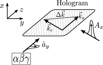
Figure 1: Illumination of the hologram by the write–in (single pass operation).

Let us introduce the difference wave vector $\Delta\vec{k}=\vec{k}_{s}-\vec{k}_{c}$ with the only non-zero projections $\Delta k_{y}$ and $\Delta k_{z}$. One can consider a thin (that is, of the width much less than $\lambda$) atomic layer orthogonal to $\Delta\vec{k}$, where the phase difference between the signal and the driving classical wave is constant. The quantum non-demolition (QND) light-matter interaction in each layer leads to two basic effects: (i) the Faraday rotation of light polarization due to quantum $z$-component of collective atomic spin of the slice; and (ii) the atomic spin rotation, caused by the unequal light shifts of the ground state sub-levels with $m_{z}=\pm 1/2$ in the presence of quantum fluctuations of circular light polarizations. The interaction within the slice is described by the well known QND Hamiltonian Hammerer10 :

$$H=\frac{2\pi k_{0}|d|^{2}}{\omega_{eg}-\omega_{0}}\int_{V}d\vec{r}\sum_{a}J_{z}^{a}(t)S_{z}(\vec{r},t)\delta(\vec{r}-\vec{r}_{a}).$$ (1)

Here $\omega_{eg}$ is the frequency of the atomic transition, $d$ is the dipole matrix element, and $k_{0}=\omega_{0}c$. For the non-copropagating signal and driving waves, the $z$-component of the Stokes vector $S_{z}(\vec{r},t)=2A_{x}\,{\rm Im}\left[A_{y}(\vec{r},t)\exp(i\Delta\vec{k}\vec{r})\right]$ in (1) slowly varies within the slice and rapidly oscillates (i.e. on the scale $1/\Delta k$) along the $\Delta\vec{k}$ direction. The slowly varying amplitude $A_{y}$ of the quantized signal field is defined via

$$A_{y}(z,\vec{\rho},t)=\int\frac{dk_{z}}{2\pi}\int\frac{d\vec{q}}{(2\pi)^{2}}\sqrt{\omega(k)/k_{0}}\,a_{y}(\vec{k})\exp[i\{\vec{q}\vec{\rho}+(k_{z}-k_{0})z-(\omega(k)-\omega_{0})t\}],$$

where $\vec{r}=(\vec{\rho},z)$, $\vec{k}=(\vec{q},k_{z})$. Here $a_{y}(\vec{k})$ and $a_{y}^{\dagger}(\vec{k})$ are the annihilation and creation operators for the wave $\vec{k}$, which obey standard commutation relations $[a_{y}(\vec{k}),a_{y}^{\dagger}(\vec{k}\,^{\prime})]=(2\pi)^{3}\delta(\vec{k}-\vec{k}\,^{\prime})$, $[a_{y}(\vec{k}),a_{y}(\vec{k}\,^{\prime})]=0$. By using these commutation relations in the paraxial approximation, one finds Kolobov99 the commutation relation for the slowly varying amplitude of the quantized signal field $A_{y}$,

$$[A_{y}(z,\vec{\rho},t),A_{y}^{\dagger}(z^{\prime},\vec{\rho}\,^{\prime},t)]\equiv c\tilde{\delta}(\vec{r}-\vec{r}\,^{\prime})\approx$$ (2)

$$c\left(1-\frac{i}{k_{0}}\frac{\partial}{\partial z}-\frac{1}{2k^{2}_{0}}\nabla^{\,2}_{\bot}\right)\delta(\vec{r}-\vec{r}\,^{\prime}).$$

We do not consider here quantized waves of other than $\vec{k}_{s}$ mean propagation directions because their evolution is independent of the signal wave under consideration.

We introduce the density of the collective spin as $\vec{J}(\vec{r})=\sum_{a}\vec{J}^{a}\delta(\vec{r}-\vec{r}_{a})$. The averaged over random positions of the atoms commutation relation for the $y$, $z$ components of the collective spin is

$$\overline{[J_{y}(\vec{r}),J_{z}(\vec{r}\,^{\prime})]}=i\sum_{a}\langle J_{x}^{a}\rangle\overline{\delta(\vec{r}-\vec{r}_{a})\delta(\vec{r}\,^{\prime}-\vec{r}_{a})}^{a}=in_{a}\langle J_{x}^{a}\rangle\delta(\vec{r}-\vec{r}\,^{\prime}).$$

Here $n_{a}$ is the average density of atoms. The field-like canonical variables for the spin subsystem,

$$X(\vec{r},t)=J_{y}(\vec{r},t)/\sqrt{n_{a}\langle J_{x}^{a}\rangle},\quad P(\vec{r},t)=J_{z}(\vec{r},t)/\sqrt{n_{a}\langle J_{x}^{a}\rangle},$$

obey the canonical commutation relation:

$$\overline{[X(\vec{r},t),P(\vec{r}\,^{\prime},t)]}=i\delta(\vec{r}-\vec{r}\,^{\prime}).$$ (3)

The full Hamiltonian of our model includes the energy of free electromagnetic field and the effective Hamiltonian of QND interaction. The Hamiltonian reads,

$$H=\int_{V}d\vec{r}\left\{\frac{\hbar\omega_{0}}{c}A_{y}^{\dagger}(z,\vec{\rho},t)\,A_{y}(z,\vec{\rho},t)\,-\right.$$ (4)

$$\left.i\frac{2\pi k_{0}|d|^{2}}{\omega_{eg}-\omega_{0}}\sqrt{n\langle J_{x}^{a}\rangle}A_{x}(z,t)P(z,\vec{\rho},t)\big{[}A_{y}(z,\vec{\rho},t)e^{i\Delta\vec{k}\vec{r}}-h.c.\big{]}\right\}.$$

We describe the evolution of our system in the Heisenberg picture. With the use of commutation relations (2) and (3) for the field and atomic variables, after simple transformations we obtain:

$$\left(\frac{\partial}{\partial z}-\frac{i}{2k_{0}}\nabla^{\,2}_{\bot}+\frac{1}{c}\frac{\partial}{\partial t}\right)A_{y}(z,\vec{\rho},t)=\frac{\tilde{\kappa}}{\sqrt{LT}}\,P(z,\vec{\rho},t)e^{-i\Delta\vec{k}\vec{r}},$$ (5)

$$\frac{\partial}{\partial t}X(z,\vec{\rho},t)=\frac{2\tilde{\kappa}}{\sqrt{LT}}{\rm Im}\left[A_{y}(z,\vec{\rho},t)e^{i\Delta\vec{k}\vec{r}}\right],\qquad\frac{\partial}{\partial t}P(z,\vec{\rho},t)=0.$$ (6)

Here $T$ is the duration of the flat-top pulse of driving field and $L$ is the atomic cell length. The dimensionless coupling constant

$$\tilde{\kappa}=\frac{2\pi k_{0}|d|^{2}}{\hbar(\omega_{eg}-\omega_{0})}\sqrt{n_{a}\langle J_{x}^{a}\rangle A_{x}^{2}LT},$$ (7)

should be of the order of unity for the memory to work (note that $\tilde{\kappa}$ is $\sqrt{2}$ times the coupling constant $\kappa$ defined in Vasilyev10 for volume hologram with rotating spins). The coupling constant can be written as ${\tilde{\kappa}}^{2}=2\alpha_{0}\eta$, where $\alpha_{0}$ is the resonant optical depth and $\eta$ is the probability of spontaneous emission Cerf07 . Since $\eta\ll 1$ is required in order to neglect the effect of spontaneous emission from the upper level, the usual condition $\alpha_{0}=\lambda^{2}n_{a}L/2\pi\gg 1$ should be fulfilled. We introduce the Fourier transform via

$$a(z,\vec{q},t)=\int d\vec{\rho}\,A_{y}(z,\vec{\rho},t)e^{-i\vec{q}\,\vec{\rho}},$$ (8)

and similar for atomic variables, and arrive to the set of basic equations in the Fourier domain:

$$\left(\frac{\partial}{\partial z}+i\frac{\vec{q}\,^{2}}{2k_{0}}+\frac{1}{c}\frac{\partial}{\partial t}\right)a(z,\vec{q},t)=\frac{\tilde{\kappa}}{\sqrt{LT}}\,p(z,\vec{q}-\Delta\vec{k}_{y},t)e^{-i\Delta k_{z}z},$$ (9)

$$\frac{\partial}{\partial t}x(z,\vec{q},t)=\frac{2\tilde{\kappa}}{\sqrt{LT}}{\rm Im}\left[a(z,\vec{q}+\Delta\vec{k}_{y},t)e^{i\Delta k_{z}z}\right],\qquad\frac{\partial}{\partial t}p(z,\vec{q},t)=0.$$ (10)

Notice that the collective spin quadrature amplitude $p$ responsible for the Faraday rotation does not evolve, similar to the case of thin quantum hologram of Vasilyev08 . Hence, this amplitude is effectively recorded into one of the signal wave quadratures within all duration $T$ of one interaction cycle.

Let us consider the following boundary condition. We position the center of atomic sample of length $L$ at $z=0$, and define the input signal wavefront $A^{(in)}(\vec{\rho},t)$ and the Fourier amplitudes $a^{(in)}(\vec{q},t)$ with respect to the central ($x$, $y$) plane at $z=0$ in free space. The actual signal field at the input cell face is related to the defined “in” amplitudes as

$$a(-L/2,\vec{q},t)=a^{(in)}(\vec{q},t)e^{i\frac{q^{2}}{2k_{0}}\frac{L}{2}}.$$ (11)

One can imagine an external lens focusing system which transfers the field $A^{(in)}(\vec{\rho},t)$ from its input plane to the plane at $z=0$, so that $A^{(in)}(\vec{\rho},t)$ is the input field of the lens system. We arrive to the following solution of the Eq. (9):

$$a(z,\vec{q},t)=a^{(in)}(\vec{q},t)e^{-i\frac{q^{2}}{2k_{0}}z}+\frac{\tilde{\kappa}}{\sqrt{LT}}\int_{-L/2}^{z}dz^{\prime}p^{(in)}(z^{\prime},\vec{q}-\Delta\vec{k}_{y})e^{-i\Delta k_{z}z^{\prime}}e^{-i\frac{q^{2}}{2k_{0}}(z-z^{\prime})},$$ (12)

where $p^{(in)}(z,\vec{q}\,)=p(z,\vec{q},0)$. We assume pulse duration $T$ to be much larger than the retardation time at the length $L$ of ensemble, $T\gg L/c$ and neglect $\sim 1/c$ term in the field evolution equation (9). The Eq. (10) yields,

$$x(z,\vec{q},t)=x^{(in)}(z,\vec{q}\,)+\frac{2\tilde{\kappa}}{\sqrt{LT}}\int_{0}^{t}dt^{\prime}\,{\rm Im}\left[a(z,\vec{q}+\Delta\vec{k}_{y},t^{\prime})e^{i\Delta k_{z}z}\right].$$ (13)

We should have in mind that the field amplitudes are defined as slow in space in dependence of $z$ coordinate, but the spin amplitudes are not. The Eqs. (12), (13) show that QND interaction with quantized field $a(z,\vec{q},t)$ produces fast spatial modulation of collective spin, and similar fast modulation is read out by the the field. The fast modulation of collective spin at spatial frequency $\Delta\vec{k}$ is just a consequence of the non-collinear geometry of our volume hologram. The volume hologram is a spatial multi–layer structure with typical spatial period of the order of $2\pi/\Delta k$. Within this spatial period, the phase difference between the signal and the driving classical wave changes by $2\pi$ and therefore changes the type of local circular polarization which is crucial for QND interaction. This imposes limitations on the atomic motion during storage time: the atoms should not transport coherence from one layer to another. A solid state, an optical lattice, or ultra cold atoms should be used.

We go over to slow amplitudes of the collective spin by compensating fast spatial oscillations present at right side of Eqs. (12), (13), and perform mode decomposition of the slow amplitudes:

$$x_{n}(\vec{q},t)\equiv\int_{-L/2}^{L/2}dz\,\theta_{n}(z)x(z,\vec{q}-\Delta\vec{k}_{y},t)e^{-i(\Delta k_{z}-\frac{q^{2}}{2k_{0}})z}.$$ (14)

The same decomposition is applied to quadrature amplitude $p(z,\vec{q}-\Delta\vec{k}_{y})$. Here

$$\theta_{n}(z)={\cal N}_{n}\sqrt{\frac{2}{L}}\,P_{n}\left(\frac{2z}{L}\right),\qquad{\cal N}_{n}=\sqrt{\frac{2n+1}{2}},$$ (15)

$P_{n}(x)$ is the n-th Legendre polynomial, $n=0,1,2,\dots$, and ${\cal N}_{n}$ is the normalization constant. A similar mode decomposition in time domain has been introduced in Hammerer06 . Some lower–order amplitudes are given by

$$x_{0}(\vec{q},t) = \sqrt{\frac{1}{L}}\int_{-L/2}^{L/2}dz\,x(z,\vec{q}-\Delta\vec{k}_{y},t)e^{-i(\Delta k_{z}-\frac{q^{2}}{2k_{0}})z},$$ (16)

$$x_{1}(\vec{q},t) = 2\left(\frac{3}{L^{3}}\right)^{1/2}\int_{-L/2}^{L/2}dz\,z\,x(z,\vec{q}-\Delta\vec{k}_{y},t)e^{-i(\Delta k_{z}-\frac{q^{2}}{2k_{0}})z},$$ (17)

$$x_{2}(\vec{q},t) = 6\left(\frac{5}{L^{5}}\right)^{1/2}\int_{-L/2}^{L/2}dz\left(z^{2}-\frac{L^{2}}{12}\right)x(z,\vec{q}-\Delta\vec{k}_{y},t)e^{-i(\Delta k_{z}-\frac{q^{2}}{2k_{0}})z}.$$ (18)

We assume that the length $L$ of atomic cell is large as compared to the wavelength. For large enough angle between the driving and the signal field wave vectors $\vec{k}_{c}$ and $\vec{k}_{s}$ (that is, a collinear geometry is not considered here) one has $\Delta k_{z}L\gg 1$. Physically this means that our volume hologram contains many interference layers discussed above.

These new amplitudes allow us to express solutions for atomic and light variables in a more compact way. As before, we define the output signal field amplitude with respect to the central $(x,y)$ plane at $z=0$. The actual signal field at the output face of the cell is

$$a(L/2,\vec{q},t)=a^{(out)}(\vec{q},t)e^{-i\frac{q^{2}}{2k_{0}}\frac{L}{2}}.$$ (19)

Here one can imagine an output lens focusing system which in free space transfers the signal field from the plane $z=0$ to its output plane. Define the averaged over the pulse duration $T$ signal amplitude as

$$a(\vec{q}\,)=\frac{1}{\sqrt{T}}\int_{T}dt\,a(\vec{q},t).$$ (20)

The field propagation equation (12) yields,

$$a^{(out)}(\vec{q}\,)=a^{(in)}(\vec{q}\,)+\tilde{\kappa}\,p_{0}^{(in)}(\vec{q}\,).$$ (21)

In order to find slow atomic amplitudes we insert (12) into (13) and make use of the definition (14). The proportional to $e^{-i\Delta k_{z}z}$ term in (13) after substitution into (14) gives rise to fast spatial oscillations, and in the limit $\Delta k_{z}L\gg 1$ vanishes by the integration over $z$. For the output slow amplitudes of the collective spin, where $x_{n}^{(out)}(\vec{q}\,)=x_{n}(\vec{q},T)$ and $p_{n}^{(out)}(\vec{q}\,)=p_{n}(\vec{q},T)$, we find

$$x_{0}^{(out)}(\vec{q}\,)=x_{0}^{(in)}(\vec{q}\,)-i\tilde{\kappa}a^{(in)}(\vec{q}\,)-i\frac{\tilde{\kappa}^{2}}{2}\left[p_{0}^{(in)}(\vec{q}\,)-\frac{1}{\sqrt{3}}p_{1}^{(in)}(\vec{q}\,)\right],$$ (22)

$$x_{n}^{(out)}(\vec{q}\,)=x_{n}^{(in)}(\vec{q}\,)-i\frac{\tilde{\kappa}^{2}}{2}\left[Q_{n,n-1}p_{n-1}^{(in)}(\vec{q}\,)+Q_{n,n+1}p_{n+1}^{(in)}(\vec{q}\,)\right],$$ (23)

where $n=1,2,\ldots\,$, and

$$p_{n}^{(out)}(\vec{q}\,)=p_{n}^{(in)}(\vec{q}\,).$$ (24)

Here the matrix $Q$ is given by

$$Q_{n,n-1}=\frac{1}{\sqrt{(2n-1)(2n+1)}},\qquad Q_{n,n+1}=-\frac{1}{\sqrt{(2n+1)(2n+3)}}.$$ (25)

While deriving (22, 23) we made use of the following property of the Legendre polynomials,

$$\int dxP_{n}(x)=\frac{1}{2n+1}[P_{n+1}(x)-P_{n-1}(x)].$$ (26)

The Eqs. (21, 22) demonstrate that by a single pass of light, the amplitude $p^{(in)}_{0}(\vec{q}\,)$ of the collective spin is read–out by the signal, and the amplitude $a^{(in)}(\vec{q}\,)$ of signal field is mapped onto the atomic amplitude $x_{0}^{(out)}(\vec{q}\,)$. One can also observe in the Eq. (22) effects of the transfer of the collective spin coherence between atomic layers in the positive $z$–direction, which are absent in the QND based thin hologram. The “active” spin amplitude $p$ produces a contribution to the quantized field $a$, which is written into the “passive” amplitude $x$ somewhere in the next layers.

By contrast to the QND based scheme of Vasilyev08 , both quadrature amplitudes of the light field are stored in a single cycle of light–matter interaction. This feature of the present scheme is related to its non–collinear geometry. One can imagine two shifted by a fraction of wavelength sub–lattices of the collective spin, so that any of two quadrature amplitudes of the signal is independently stored in the relevant sublattice.

In some sense a single–pass storage and a single–pass retrieval of the signal light state is achieved in the present scheme. After the first (the write–in) cycle of interaction one has to rotate the spins by $\pi/2$ relative the $x$–axis, so that the initial condition for the second (the read–out) cycle is given by

$$p_{n}^{R(in)}(\vec{q}\,)=x_{n}^{W(out)}(\vec{q}\,),$$ (27)

and let another light pulse to read–out the stored state. By applying twice the in–out transformations (21, 22), we find for the output light amplitude:

$$a^{R(out)}(\vec{q}\,)=-i\tilde{\kappa}^{2}a^{W(in)}(\vec{q}\,)+a^{R(in)}(\vec{q}\,)+\tilde{\kappa}x_{0}^{W(in)}(\vec{q}\,)-i\frac{\tilde{\kappa}^{3}}{2}\left[p_{0}^{W(in)}(\vec{q}\,)-\frac{1}{\sqrt{3}}p_{1}^{W(in)}(\vec{q}\,)\right].$$ (28)

What we have achieved so far is a classical volume hologram. Given $\tilde{\kappa}=1$, this result yields the initial quantized signal field $a^{W(in)}(\vec{q}\,)$ restored with proper amplitude, but quantum fluctuations of initial amplitudes of the atoms and the read–out light degrade the fidelity of memory below classical limit. The problem comes from the fact that the light and matter subsystems do not “forget” their initial states during the interaction.

III Double pass quantum volume hologram

The double pass operation of our volume hologram looks similar to the case of the QND based thin hologram. In order to compensate initial noise terms and to go beyond the classical limit, we introduce at the writing stage the second pass through the atomic sample of both (the signal and the classical) light waves in the same directions $\vec{k}_{s}$ and $\vec{k}_{c}$. After the first pass one has to rotate the spins around the $x$-axis by $\pi/2$ pulse of auxiliary magnetic field, and to apply phase shift of $\pi/2$ to the output signal wave relative the classical driving wave within the interaction volume. The transformation of light and matter variables between the first and the second pass, which is described by the same equations as before, is given by

$$a^{W(2,in)}(\vec{q}\,)=ia^{W(1,out)}(\vec{q}\,),\quad x_{n}^{W(2,in)}(\vec{q}\,)=-p_{n}^{W(1,out)}(\vec{q}\,),\quad p_{n}^{W(2,in)}(\vec{q}\,)=x_{n}^{W(1,out)}(\vec{q}\,).$$ (29)

After all three steps of the write-in procedure we arrive to the following in–out relations for the double–pass operation:

$$a^{W(out)}(\vec{q}\,)=i(1-\tilde{\kappa}^{2})a^{W(in)}(\vec{q}\,)+i\tilde{\kappa}\left(1-\frac{\tilde{\kappa}^{2}}{2}\right)p_{0}^{W(in)}(\vec{q}\,)+\tilde{\kappa}x_{0}^{W(in)}(\vec{q}\,)+i\frac{\tilde{\kappa}^{3}}{2\sqrt{3}}p_{1}^{W(in)}(\vec{q}\,),$$ (30)

$$x_{0}^{W(out)}(\vec{q}\,)=\tilde{\kappa}\left(1-\frac{\tilde{\kappa}^{2}}{2}\right)a^{W(in)}(\vec{q}\,)-\left(1-\tilde{\kappa}^{2}+\frac{\tilde{\kappa}^{4}}{6}\right)p_{0}^{W(in)}(\vec{q}\,)-i\frac{\tilde{\kappa}^{2}}{2}\left[x_{0}^{W(in)}-\frac{1}{\sqrt{3}}x_{1}^{W(in)}\right]+$$

$$\frac{\tilde{\kappa}^{4}}{4}\left[\frac{1}{\sqrt{3}}p_{1}^{W(in)}(\vec{q}\,)-\frac{1}{3\sqrt{5}}p_{2}^{W(in)}(\vec{q}\,)\right],$$ (31)

and

$$p_{0}^{W(out)}(\vec{q}\,)=x_{0}^{W(in)}(\vec{q}\,)-i\tilde{\kappa}a^{W(in)}(\vec{q}\,)-i\frac{\tilde{\kappa}^{2}}{2}\left[p_{0}^{(in)}(\vec{q}\,)-\frac{1}{\sqrt{3}}p_{1}^{(in)}(\vec{q}\,)\right],$$ (32)

$$p_{1}^{W(out)}(\vec{q}\,)=x_{1}^{W(in)}(\vec{q}\,)-i\frac{\tilde{\kappa}^{2}}{2}\left[\frac{1}{\sqrt{3}}p_{0}^{W(in)}(\vec{q}\,)-\frac{1}{\sqrt{15}}p_{2}^{W(in)}(\vec{q}\,)\right].$$ (33)

The double pass read–out procedure looks similar and is described by the Eqs. (30–33), where one has to substitute the label W to R.

We have omitted expressions for higher–order spin amplitudes because the output amplitude of the signal wave by the read–out $a^{R(out)}(\vec{q}\,)$ is decoupled from these observables, as seen from the Eq. (30). The result (30) also shows that both by the double pass write–in and the read–out, the output signal wave amplitude is completely independent of the input wave if the coupling constant is chosen to be $\tilde{\kappa}=1$, which is one of conditions for efficient state exchange between light and matter. In this sense our present model works as the thin quantum hologram of Vasilyev08 , where by the first pass the input signal amplitude is imprinted into the collective spin wave. After the transformation given by the Eq. (29) and the second pass, the relevant collective spin amplitude effectively cancels the input signal contribution to the output quantized field.

At the same time, the initial state of light is stored in the collective spin amplitudes $x_{0}^{W(out)}$ and $p_{0}^{W(out)}$. As a result of the atom-light interaction during two passes with properly adjusted coupling constant we have the write stage completed. Atoms and light have exchanged their initial quantum states.

In order to read out the memory one has to repeat the procedure. The output quantized field amplitude for the whole write–in and read–out cycle is found by using the W(out) amplitudes as the R(in) variables. Finally we arrive to

$$a^{R(out)}(\vec{q}\,)=\tilde{\kappa}^{2}(2-\tilde{\kappa}^{2})a^{W(in)}(\vec{q}\,)+i(1-\tilde{\kappa}^{2})a^{R(in)}(\vec{q}\,)-\tilde{\kappa}\left(1-\frac{3\tilde{\kappa}^{2}}{2}+\frac{\tilde{\kappa}^{4}}{3}\right)p_{0}^{W(in)}(\vec{q}\,)+$$

$$i\tilde{\kappa}(1-\tilde{\kappa}^{2})x_{0}^{W(in)}(\vec{q}\,)+i\frac{\tilde{\kappa}^{3}}{\sqrt{3}}x_{1}^{W(in)}(\vec{q}\,)-\frac{\tilde{\kappa}^{3}}{2\sqrt{3}}(1-\tilde{\kappa}^{2})p_{1}^{W(in)}(\vec{q}\,)-\frac{\tilde{\kappa}^{5}}{6\sqrt{5}}p_{2}^{W(in)}(\vec{q}\,).$$ (34)

One optimizes the memory performance by choosing the coupling constant $\tilde{\kappa}=1$. The input and the output variables of the total write–readout protocol of the volume quantum hologram are related as

$$a^{R(out)}(\vec{q}\,)=a^{W(in)}(\vec{q}\,)+f(\vec{q}\,),$$ (35)

where $f(\vec{q}\,)$ is the added noise term. This transformation is analogous to the one describing quantum holographic teleportation of an optical image Sokolov01 ; Gatti04 and the thin quantum hologram of Vasilyev08 . The noise contributions specific for our model of memory is given by

$$f(\vec{q}\,)=\frac{i}{\sqrt{3}}x_{1}^{W(in)}(\vec{q}\,)+\frac{1}{6}p_{0}^{W(in)}(\vec{q}\,)-\frac{1}{6\sqrt{5}}p_{2}^{W(in)}(\vec{q}\,),$$ (36)

where we assume $\tilde{\kappa}=1$. We perform the backward Fourier transform $\vec{q}\to\vec{\rho}$ and arrive at

$$A^{R(out)}(\vec{\rho}\,)=A^{W(in)}(\vec{\rho}\,)+F(\vec{\rho}\,),\qquad F(\vec{\rho}\,)\equiv\frac{1}{\sqrt{2}}[F_{X}(\vec{\rho}\,)+iF_{P}(\vec{\rho}\,)],$$ (37)

where we apply the same definition of real (Hermitian) noise quadrature amplitudes $F_{X,P}(\vec{\rho}\,)$ as in Vasilyev08 . Consider orthogonal pixellized spatial modes associated with the field amplitudes averaged over the surface $S_{j}$ of square pixel $j=1,\ldots,N$ of area $S$. The averaged noise quadrature amplitudes and the noise covariance matrix are defined via

$$F_{X,P}(j)=\frac{1}{\sqrt{S}}\int_{S_{j}}d\vec{\rho}\,F_{X,P}(\vec{\rho}\,),$$ (38)

$$C^{X}(i,j)=\langle F_{X}(i)F_{X}(j)\rangle,\qquad C^{P}(i,j)=\langle F_{P}(i)F_{P}(j)\rangle.$$ (39)

The collective spin noise quadrature amplitudes look like

$$\frac{1}{\sqrt{2}}F_{X}(j)=-\frac{1}{\sqrt{3}}{\rm Im}X_{1}^{W(in)}(j)+\frac{1}{6}{\rm Re}P_{0}^{W(in)}(j)-\frac{1}{6\sqrt{5}}{\rm Re}P_{2}^{W(in)}(j),$$ (40)

$$\frac{1}{\sqrt{2}}F_{P}(j)=\frac{1}{\sqrt{3}}{\rm Re}X_{1}^{W(in)}(j)+\frac{1}{6}{\rm Im}P_{0}^{W(in)}(j)-\frac{1}{6\sqrt{5}}{\rm Im}P_{2}^{W(in)}(j).$$ (41)

As seen from the Eq. (14), the real and the imaginary part of the amplitudes $X_{n}$ can be related to real quadrature amplitudes $X_{n,c}$ and $X_{n,s}$ of the longitudinal collective spin modes whose spatial profile is given by

$$\sqrt{2}\,\theta_{n}(z)\cos\left[\left(\Delta k_{z}-\frac{q^{2}}{2k_{0}}\right)z\right],\qquad\sqrt{2}\,\theta_{n}(z)\sin\left[\left(\Delta k_{z}-\frac{q^{2}}{2k_{0}}\right)z\right].$$

We arrive to

$${\rm Re}X_{n}(j)=\frac{1}{\sqrt{2}}X_{n,c}(j),\qquad{\rm Im}X_{n}(j)=-\frac{1}{\sqrt{2}}X_{n,s}(j),$$ (42)

and similar definitions are applied to the amplitudes $P_{n}$. In the limit of large number of the interference layers disused above, $|\Delta k_{z}L|\gg 1$, the “$\sin$” and “$\cos$” modes are orthogonal and correspond to independent degrees of freedom of the spin coherence.

The quality of quantum state transfer $|\psi^{(in)}\rangle\to|\psi^{(out)}\rangle$ is quantified via the fidelity parameter $F=|\langle\psi^{(in)}|\psi^{(out)}\rangle|^{2}$. Assume the input signal field to be in a spatially multimode coherent state. For the image field in a coherent state, decomposed over $N$ pixellized modes, the fidelity is given Gatti04 by

$$F_{N}=\left[{\rm det}\{\delta_{ij}+C^{X}(i,j)\}\,{\rm det}\{\delta_{ij}+C^{P}(i,j)\}\right]^{-1/2}.$$ (43)

We evaluate the noise covariance matrix assuming all longitudinal and transverse modes of the collective atomic spin to be initially in vacuum state, $\langle\left(X_{n,i}^{W(in)}(j)\right)^{2}\rangle=\langle\left(P_{n,i}^{W(in)}(j)\right)^{2}\rangle=1/2$, where $i=c,s$. This yields,

$$C^{X}(i,j)=C^{P}(i,j)=\frac{11}{60}\delta_{ij},\qquad F_{N}=\left(\frac{60}{71}\right)^{N}.$$ (44)

As shown in Gatti04 , the fidelity of quantum state transfer for simple multipixel arrays scales approximately as the $N$-th power of the quantity which is called average fidelity per pixel, $F_{av}=(F_{N})^{1/N}$. For the input signal prepared in a multipixel coherent state we obtain the average fidelity per pixel $F_{av}\approx 0.845$ for the whole write-in and read-out cycle of our quantum hologram. This is significantly higher than the classical benchmark $F_{av}=1/2$ for the holographic storage of an optical image in multipixel coherent state, and than the limit of $F_{av}=2/3$ on quantum cloning.

Theoretically, in order to achieve better fidelity one could perform squeezing of each of the added noise quadrature amplitudes in (36). Given perfect squeezing, which we do not consider here, this would lead to maximum fidelity $F_{av}\to 1$.

The optimal value of the coupling constant $\tilde{\kappa}=1$ corresponds to $\kappa=\sqrt{2}$ for the quantum volume hologram of Vasilyev10 , which gives there the storage and retrieval efficiency of $0.10-0.15$. This is significantly less than the non-zero quantum capacity limit on the efficiency of $0.5$ and leads, by such a low value of the coupling constant, to performance on a par with a classical hologram only. It should be noted that the experimentally achievable atomic samples have spatially dependent distribution of atomic density. The required homogeneous coupling constant could be obtained by choosing a proper transversal profile of the classical driving wave.

The resolving power in space of the double–pass quantum hologram can be characterized by a number of transverse modes (pixels), effectively stored and retrieved in the memory. Similar to the quantum volume hologram of Vasilyev10 and the spatially resolving Raman memories Golubeva10 , by the write–in and read–out in the same direction the diffraction does not modify the light–matter interaction and does not impose limitations on the resolving power which is finally determined by the sample geometry: the effectively stored orthogonal modes should propagate within the atomic ensemble. Note that the diffraction by propagation at the cell length can be compensated by thin lenses, and our definitions (11, 19) of the input and output field amplitudes account for this compensation in explicit form. The estimate of the number of stored modes given in Vasilyev10 applies to the scheme considered here as well.

IV Conclusion

We have elaborated a novel version of spatially multimode quantum memory for light – double pass quantum hologram. Similar to our previous proposals of thin quantum hologram Vasilyev08 and volume quantum hologram Vasilyev10 , the present scheme can be considered as an extension of classical holograms into the quantum domain. In our scheme, different spatial modes of the incoming field are stored in the corresponding orthogonal spatial modes of the long–lived collective spin of an ensemble of ultra–cold atoms in absence of spin rotation in external magnetic field. The double pass quantum volume hologram inherits some features of the thin and the volume quantum hologram. It is able to store transverse modes of an input light signal with the same high density as the quantum volume hologram and the Raman memories do, and it requires a fixed and relatively low optical depth as the thin hologram does. On the other hand, both the write–in and the read–out cycles of the double pass quantum hologram require two passes of light, and for a high fidelity storage (with the average fidelity per pixel exceeding $0.845$), preparation of the collective spin in a quadrature squeezed state is also required. Although we considered spin $1/2$ atoms, our analysis can be in principle applied to alkali atoms provided that the optical detuning significantly exceeds the excited state hyperfine splitting Hammerer10 .

This research has been funded by the European Commission FP7 under the grant agreement n 221906, project HIDEAS. The authors also acknowledge the support of the Russian Foundation for Basic Research under the projects 08-02-00771 and 08-02-92504. Part of the research was performed within the framework of GDRE “Lasers et techniques optiques de l’information”.

References

- (1) D. V. Vasilyev, I. V. Sokolov, and E. S. Polzik, Phys. Rev. A 81, 020302(R) (2010).
- (2) D. V. Vasilyev, I. V. Sokolov, and E. S. Polzik, Phys. Rev. A 77, 020302(R) (2008).
- (3) K. Hammerer, A. S. Sørensen, E. S. Polzik, Rev. Mod. Phys. 82(2), 1041 (2010).
- (4) Pieter Kok, W.J. Munro, Kae Nemoto, T.C. Ralph, Jonathan P. Dowling, G.J. Milburn, Rev. Mod. Phys. 79, 135 (2007).
- (5) C. Simon, H. de Riedmatten, M. Afzelius, N. Sangouard, H. Zbinden, and N. Gisin, Phys. Rev. Lett. 98, 190503 (2007).
- (6) Yu. N. Denisyuk, Dokl. Akad. Nauk SSSR 144(6), 1275 (1962) [Sov. Phys. Doklady 7, 543 (1962)].
- (7) J. Nunn, I. A. Walsmley, M. G.Raymer, K. Surmacz, F. C. Waldermann, Z. Wang, and D. Jaksch, Phys. Rev. A 75, 011401(R) (2007).
- (8) O. S. Mishina, D. V. Kupriyanov, J. H. Muller, and E. S. Polzik, Phys. Rev. A 75, 042326 (2007).
- (9) K. Surmacz, J. Nunn, K. Reim, K. C. Lee, V. O. Lorenz, B. Sussman, I. A. Walmsley, and D. Jaksch, Phys. Rev. A 78, 033806 (2008)
- (10) J. Nunn, K. Reim, K. C. Lee, V. O. Lorenz, B. J. Sussman, I. A. Walmsley, and D. Jaksch, Phys. Rev. Lett. 101, 260502 (2008).
- (11) T. Golubeva, Yu. Golubev, O. Mishina, A. Bramati, J. Laurat, E. Giacobino, ArXiv:1012.5016v2 [quant-ph] (2010).
- (12) M. I. Kolobov, Rev. Mod. Phys. 71, 1539 (1999).
- (13) K. Hammerer, J. Sherson, B. Julsgaard, J. I. Cirac, andE. S. Polzik, chapter in the book: Quantum Information with Continuous Variables of Atoms and Light, edited by N. J. Cerf, G. Leuchs, and E. S. Polzik (Imperial College Press, 2007).
- (14) K. Hammerer, E. S.Polzik, and J. I. Cirac, Phys. Rev. A 74, 064301 (2006).
- (15) I. V. Sokolov, M. I. Kolobov, A. Gatti, L. A. Lugiato, Opt. Comm. 193, 175 (2001).
- (16) A. Gatti, I. V. Sokolov, M. I. Kolobov and L. A. Lugiato, Eur. Phys. J. D 30, 123 (2004).
- (17) A. Kuzmich and E. S. Polzik, chapter in the book: Quantum Information with Continuous Variables, edited by S. Brainstein and A. Pati (Kluwer, 2003).
- (18) J. Sherson, B. Julsgaard, and E. S. Polzik, Advances in Atomic Molecular and Optical Physics 54, Academic Press (November, 2006).