Comparing partial-wave amplitude parametrization with dynamical models of meson-nucleon scattering

Abstract

Relationships between partial-wave amplitude parametrizations, in particular the Chew-Mandelstam approach, and dynamical coupled-channel models are established and investigated. A bare pole corresponding to the $\Delta(1232)$ resonance, found in a recent dynamical-model fit to $\pi-$ and $\omega-$meson production reactions, compares closely to one found in a unitary multichannel partial-wave amplitude parametrization of SAID. The model dependence of the bare pole precludes a direct connection between the approaches but is suggestive that the dynamical description and the phenomenological parametrization are closely related.

I Introduction

In this study, we outline both qualitative and quantitative relationships between dynamical models and the SAID approach to fitting meson production reactions. The SAID parametrization is based on a Chew-Mandelstam (CM) approachBabelon et al. (1976); Basdevant and Berger (1979) that has been extensively applied in multichannel descriptions of hadronically and electromagnetically induced reactions on the protonArndt et al. (1985, 1990, 1995, 2002, 2004, 2006); Prakhov et al. (2005). We compare this with recent multichannel dynamical model descriptions that assume a set of well established $N$ and $\Delta$ resonances.

Meson scattering and production reactions (collectively, “reactions”) account almost entirely for information available on the resonance structure of the nucleon. The resonances of the nucleon encode a wealth of information on the non-perturbative regime of quantum chromodynamics, the fundamental non-Abelian quantum field theory of quarks and gluons, that is responsible for nuclear forces and the interactions of effective hadronic degrees-of-freedom. Here we elaborate on the connections between well-known and widely used multichannel parametrization approaches, and dynamical model approaches, which both satisfy unitarity at the two-body level.

An issue of recent debateDoring et al. (2009) has been the interplay of singularities arising from the iteration of colloquially termed “non-pole” or “nonresonant” interactions and those explicitly added as bare states. Within the CM approach, one may askSvarc (2008) whether the inclusion of poles in the Chew-Mandelstam $K$ matrix is required. The relation between CM and Heitler $K$-matrixHeitler (1941) poles has also been studiedWorkman et al. (2009).

The present SAID fits to pion-nucleon scattering and eta-nucleon production data are based on multichannel amplitudesArndt et al. (2006) for which, with the single exception of the $P_{33}$ partial wave, the CM $K$ matrix, $\overline{K}$ has been constructed as a low-order polynomial in the center-of-mass complex scattering energy, $E$, without poles. This construction may, however, yield a pole in the Heitler $K$ matrixParis and Workman (2010), given the relationship between $K$, the Heitler $K$ matrix, and $\overline{K}$, the CM $K$ matrix:

$$K(E) =\overline{K}(E)\frac{1}{1-\mbox{Re }\!C(E)\overline{K}(E)},$$ (1)

where $C(E)$ is termed the Chew-Mandelstam ‘function,’Basdevant and Berger (1979) a diagonal matrix in the space of included channels. Evidently, poles may be located at real values of the scattering energy, $W=\mbox{Re }\!E$ when $\det[1-\mbox{Re }\!C\overline{K}]=0$Paris and Workman (2010). A strong feature of the CM approach then is that the unstable ‘particles’ (identified with the baryon resonances) of the theory arise dynamically, in a sense, from the proper analytic form of the CM parametrization in the process of fitting to the observed data in the physical region, $W=\mbox{Re }\!E>0$. The unstable particles are identified as poles of the $T$ matrix near the physical region.

One may still include explicit poles in $\overline{K}$ as is done in the $P_{33}$ partial wave of Ref.Arndt et al. (2006). If poles are present in $\overline{K}$, how should they be interpreted? A more involved question might ask for the effect of adding explicit CM $K$-matrix poles in partial waves reproducing data without their inclusion. Here, we restrict our discussion to the elastic $P_{33}$ partial wave in the $\Delta(1232)$ resonance region. This partial wave has both explicit CM and Heitler $K$-matrix poles and we compare them to structures seen in a particular dynamical model.

In Section II we discuss general features of each approach, while details are referred to in the literature. Section III contains a discussion of the results, possible extensions to this work, and conclusions.

II Model and parametrization approaches

This study is motivated in part by the observation that bare resonance parameters of a recent SAID parametrization Arndt et al. (2006) compare closely with those of recent dynamical model calculationsJulia-Diaz et al. (2007); Paris (2009). The first subsection deals with details of the dynamical model and the Chew-Mandelstam parametrization approaches relevant to understanding this comparison. The second subsection gives a more general discussion of dynamics in the model and parametrization approaches.

II.1 Dynamical model

We limit our discussion of the dynamical coupled-channel approaches to the general features relevant to describing bare resonance parameters. In this work, we study these model-dependent quantities and their relation to physical, dressed resonance poles in the scattering, $S$ or transition, $T$ matrices. Details of the dynamical model can be found elsewhereJulia-Diaz et al. (2007); Paris (2009).

The reaction observables are determined by the matrix elements of the transition operator, $T$, a matrix in momentum, spin, and channel spaces. The dynamical approach makes a model-dependent separation into ‘nonresonant’ and ‘resonant’ contributions:

$$T(E) =t(E)+t^{R}(E).$$ (2)

Since the total $T$ matrix satisfies the (relativistic) Lippmann-Schwinger equation

$$T(E) =V+VG_{0}(E)T(E)$$ (3)

where $V$ is the (relativistic) tree-level interaction kernel, $G_{0}=[E-H_{0}]^{-1}$ is the many-body free particle propagator for the free particle Hamiltonian, $H_{0}$ with physical masses, and $E\in\mathbb{C}$ is the complex scattering energy, the nonresonant and resonant contributions satisfy

$$t(E) =v+vG_{0}(E)t(E),$$ (4)

$$t^{R}(E) =\overline{\Gamma}^{\dagger}(E)\frac{1}{E-H_{0}-\Sigma(E)}\overline{\Gamma}(E),$$ (5)

respectively. Here, $v$ is the non-resonant contribution to $V$, $\overline{\Gamma}(\overline{\Gamma}^{\dagger})$ is the $MB\to B^{\prime}$($B\to MB^{\prime}$) dressed vertex, $M$ and $B$ are meson and baryon fields, $\Sigma(E)=\Gamma G_{0}(E)\overline{\Gamma}^{\dagger}(E)$ is the baryon self-energy, and $\Gamma$ is the bare vertex. (Here, the ${\dagger}$ symbol is not Hermitian conjugation. It simply distinguishes $MB\to B^{\prime}$ from the inverse process.) The dressed vertex is related to the bare vertex as $\overline{\Gamma}=\Gamma(1+G_{0}t(E))$. The resonances of the dynamical model are determined by locating the set of complex energies $\{E_{r}\}_{r=1}^{N_{R}}$ where

$$\det[E_{r}-(M^{(0)}+\Sigma(E_{r}))] =0,$$ (6)

corresponding to poles of the $T$ (or $S$) matrix. Here $N_{R}$ is the number of energies in a given partial wave for which the above equation is satisfied. We note in passing that the number of resonance poles need not be equal to the number of bare states with real energies $M^{(0)}_{i}$Suzuki et al. (2010), where $i$ indexes one specific, of a number of assumed, bare one-particle intermediate states. We note that for the $P_{33}$ partial wave the poles of $T$ and the poles of $t^{R}$ are identical since there are no poles in the non-resonant part $t$. The pole mass, $M_{r}$ and total width, $\Gamma_{r}$ of the baryon resonance are related to the pole position, $E_{r}$ as

$$M_{r} =\mbox{Re }\!E_{r},$$ (7)

$$-{\tfrac{1}{2}}\Gamma_{r} =\mbox{Im }\!E_{r},$$ (8)

which are complicated functions of the bare parameters of the Lagrangian. The bare mass, $M^{(0)}_{i}$ is dressed by interaction with the meson and baryon fields of the Lagrangian.

It is appropriate to reiterate caveats associated with the bare parameters of reaction theories in general and the particular dynamical coupled-channel approach described here. There are several features of the dynamical approach that are model dependent and for which extensive studies to quantify the precision of model predictions are lacking. For example, there are no quantitative studies, to our knowledge, that specify the accuracy of the bare parameters of the Lagrangian within a given model approach, including the bare resonance mass and width. The origin of the model dependence in the dynamical approach stems, in part, from the application of the calculational device of decomposing the $T$ matrix in Eq.(2) into two terms called, colloquially, nonresonant and resonant. The model dependence of this decomposition may be viewed as a consequence of the field redefinition ambiguities of the effective quantum field theory that describes the hadronic degrees-of-freedom. As shown in Ref.Gegelia and Scherer (2010), a field redefinition may be applied, for example, to transform a heavy fermion field operator. This has the effect of shifting strength between nonresonant and resonant mechanisms while leaving invariant the observables of the theory. The resonance parameters, however, depend on the field redefinition and therefore cannot be observables. We also reiterate the fact that the CM parametrization approach makes no such decomposition of the $T$ matrix into nonresonant or resonant contributions. Therefore, it is free of model dependencies that arise in such a decomposition.

We have, nevertheless, noticed a close numerical match between the bare value of the bare pole position in the dynamical model and explicitly included CM $K$ matrix pole in the $P_{33}$ partial wave of the parametrization employed in Ref.Arndt et al. (2006). In the next subsection we analyze this result in terms of the structure of the CM parametrization form. Our hope is that by analyzing the structure of both the model and parametrization forms and studying their relationships that we may learn more about the nature of the dynamics included within each approach.

II.2 Chew-Mandelstam approach

We give a brief description of the CM parametrization form here. More complete discussions of the form and its application to the determination of the partial wave amplitudes in the multichannel hadro- and photoproduction observed data are described in the literatureBabelon et al. (1976); Basdevant and Berger (1979); Paris and Workman (2010)

The unitarity of the $S$ matrix implies a constraint, called “unitarity,” on the $T$ matrix, which may be concisely expressed as:

$$\mbox{Im }\!T^{-1}(E) =-\rho(E),$$ (9)

where $\rho=-\pi\delta(E-H_{0})$ and the relationship between $T$ and $S$ is given by $S=1+2i\rho T$. This implies that the full $T$ matrix satisfies the Heitler equation:

$$T(E) =K(E)+iK(E)\rho(E)T(E),$$ (10)

where $K^{-1}\equiv\mbox{Re }\!T^{-1}$. The Heitler $K$ matrix, $K$, has the features of being a real-symmetric matrix in channel space and of being free of threshold branch point singularitiesZimmerman (1961). The Heitler $K$ matrix expressed in terms of the CM $K$ matrix, $\overline{K}$ is

$$K^{-1}(E) =\overline{K}^{-1}(E)-\mbox{Re }\!C(E),$$ (11)

where $\mbox{Re }\!C$ is the Hilbert transform of $\rho$ (with one subtraction). Solving for $K$ in the above relation yields Eq.(1). Parametrization of the matrix elements of $\overline{K}$ as functions analytic in the finite complex $E$-plane yield, in general, matrix elements of $K$ that are meromorphic in the energy. The $K$-matrix poles that arise in this manner are sometimes related to the poles of the $T$ matrix. This connection has been explored in Ref.Workman et al. (2009). The $T$ matrix may then be expressed as

$$T(E) =\overline{K}(E)+\overline{K}(E)C(E)T(E)$$ (12)

directly in terms of the CM $K$ matrix.

Having established the representation of the $T$ matrix in terms of the parametrized function $\overline{K}$ we consider the form of its matrix elements which include a single explicit pole. The $\overline{K}$ matrix is then written as

$$\overline{K} =\frac{\gamma}{W-W_{p}}+\beta(W),$$ (13)

where $\gamma$ is a constant matrix in channel space and $\beta(W)$ is an analytic matrix function of $W$, typically a polynomial. This is, in fact, the form of the CM $K$ matrix used in Ref.Arndt et al. (2006) for the $P_{33}$ partial wave. Our fit to the complete $\pi N$ elastic and $\pi N\to\eta N$ reaction data gives, for the pole position of the CM $K$ matrix,

$$W_{p}(P_{33}) =1381\mbox{ MeV}.$$ (14)

The position of the Heitler $K$-matrix pole in the SAID $P_{33}$ parametrization is related the CM $K$ matrix pole as:

$$W_{p}^{H}(P_{33})=W_{p}(P_{33})+\frac{\gamma_{\pi N,\pi N}\mbox{Re }\!C_{\pi N}}{1-\beta_{\pi N,\pi N}\mbox{Re }\!C_{\pi N}}$$ (15)

where, $C_{\pi N}$ is the elastic, $\pi N$ matrix element of the CM function. The position of the Heitler $K$-matrix pole isWorkman et al. (2009)

$$W_{p}^{H}(P_{33}) =1232\mbox{ MeV}$$ (16)

and is essentially model-independentDavidson and Mukhopadhyay (1990). Energy-dependent quantities in Eq.(15) are evaluated at the Heitler $K$ matrix pole.

The fact that both the Heitler $K$ matrix, $K$, and the CM $K$ matrix, $\overline{K}$, have poles on the physical region at $W^{H}_{p}(P_{33})=1232$ MeV and $W_{p}(P_{33})=1381$ MeV, respectively, constrains the real part of $T_{\pi N,\pi N}(W^{H}_{p}(P_{33}))$ and the Chew-Mandelstam function, $C_{\pi N}(W_{p}(P_{33}))$. Employing Eqs.(10) and (12) for energies below the point at which inelastic channels become important, $W\lesssim 1450$ MeV (see Fig.(2), below) and taking the imaginary part gives the following expression:

$$K_{\pi N,\pi N}(W)\,\mbox{Re }\!T_{\pi N,\pi N}(W)=\overline{K}_{\pi N,\pi N}(W)$$

$$\times\left[\frac{\mbox{Re }\!C_{\pi N}(W)}{\rho_{\pi N}(W)}\mbox{Im }\!T_{\pi N,\pi N}(W)+\mbox{Re }\!T_{\pi N,\pi N}(W)\right].$$ (17)

Note that this relation holds in the elastic region only. This relation provides constraints at the pole positions $W^{H}_{p}$ and $W_{p}$ (where the $\pi N$ partial wave designation, $P_{33}$ is to be understood from here forward):

$$\mbox{Re }\!T_{\pi N,\pi N}(W^{H}_{p}) =0$$ (18)

$$\tan\delta_{\pi}(W_{p})+\frac{\rho_{\pi N}(W_{p})}{\mbox{Re }\!C_{\pi N}(W_{p})} =0,$$ (19)

which are satisfied at the values given in Eqs.(14) and (16), respectively. Here, $\tan\delta_{\pi}=\mbox{Im }\!T_{\pi N,\pi N}/\mbox{Re }\!T_{\pi N,\pi N}$ is determined by the elastic $\pi N\to\pi N$ $P_{33}$ phase shift. Variability in the pole position is therefore directly linked to our determination of $\mbox{Re }\!C_{\pi N}(W)$ and, conversely, the determination of $C_{\pi N}(W_{p})$ must satisfy the constraint of Eq.(19); it is not model dependent. As the SAID parametrization of $\mbox{Re }\!C_{\pi N}(W)$ is fixed, apart from a subtraction determining its zero point, and this value is not searched, the pole position has remained essentially constant for different SAID solutions even as new data and dispersion-relation constraints were added. We also note that the $T$-matrix values at the Heitler $K$-matrix pole, $T_{\pi N,\pi N}(W^{H}_{p})=i$, and at the CM $K$-matrix pole, $T_{\pi N,\pi N}(W_{p})=-\rho_{\pi N}(W_{p})/C_{\pi N}(W_{p})$, are independent of the $K$-matrix parametrization. A note of caution may be appropriate here: Eq.(18) appears similar to the condition for locating the real part of the pole position of a Breit-Wigner parametrization. We hope, however, that the preceding discussion makes clear that the position of the Heitler $K$ matrix pole bares no simple relation to model dependent and generally non-unitary Breit-Wigner parametrization.

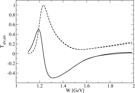
Figure 1: Comparison of the SP06 $P_{33}$ partial wave elastic $T$ matrix elementArndt et al. (2006) (dimensionless) having a sum of pole and non-pole $K$-matrix elements, and a fit using the product $S$-matrix form, FP10. The plotted real (solid) and imaginary (dashed) parts are virtually identical over the resonance region, producing equivalent fits to data.

If $\beta_{\pi N,\pi N}$ is set to zero and the $T$-matrix pole position recalculated, its value shifts to $1297-i24$ MeV. Clearly the pole and non-pole terms at the CM $K$-matrix level do not translate directly into resonant and nonresonant contributions to the $T$ matrix. This separation is possible, phenomenologically, if one instead parametrizes the $S$ matrix as $S_{B}S_{R}S_{B}$ with the resonance $T$ matrix, giving $S_{R}$, fitted as above but with $\beta_{\pi N,\pi N}$ set to zero. The $S_{B}$ is then similarly constructed with $\gamma_{\pi N,\pi N}$ set to zero. A fit to data using this form, FP10, has been completedWorkman and Paris (2010) and is plotted against the standard form (SP06) in Fig.(1). The resulting Heitler $K$-matrix and $T$-matrix poles are found at 1232 MeV and $1211-i50$ MeV respectively, as in the original fit. The CM $K$-matrix pole shifts, in this case, to 1480 MeV. Here, however, setting the “background” to zero (ie., $S_{B}\to 1$) has no effect on the $T$-matrix pole position.

At higher energies, many resonances can be discovered by searching for poles in the complex energy plane, without the explicit introduction of CM $K$-matrix poles. It would be interesting to consider the effect of adding explicit poles to resonant partial waves of this type. The resulting interplay of pole and non-pole contributions could add new structures or replace resonances, generated by non-pole terms, with pole-generated structures.

II.3 Comparison of dynamical model and CM parametrization

Turning to the comparison of the dynamical model with the SAID CM parametrization, Refs. Paris (2009) and Suzuki et al. (2010) give the values of bare resonance parameters in their Tables VI and II, respectively. The value for the $P_{33}$ resonance is given as

$$M^{(0)}(P_{33}) =1391\mbox{ MeV}.$$ (20)

The numerical similarity to $W_{p}(P_{33})$ suggests a close relationship between a dynamical coupled-channel approach and the CM $K$-matrix parametrization.

It can be effectively argued that the essentially elastic nature of the $P_{33}$ partial wave and the fact that nonresonant effects are small in the region of the $P_{33}(1232)$ resonance are specific, perhaps, only to this particular partial wave. We would not dispute this claim. The purpose of the present comparison, however, is to indicate that the dynamics of rescattering, including final-state interactions and coupled-channel effects, are included in an essential way into the CM parametrization. In the specific case of the $P_{33}$ partial wave, which provides a simple case study, there is a quantitative verification of this fact given by Eq.(20). We elaborate on this point further by analyzing and comparing the rescattering effects in the model and parametrization approaches.

There are two distinct sources of rescattering effects which dress the explicit pole in the CM parametrization. The first, comes about in Eq.(1), where the real part of the Chew-Mandelstam function, $\mbox{Re }\!C$ reflects the off-shell propagation of the intermediate two-particle states. In fact, the subtraction constant in $C$Paris and Workman (2010) reflects the model dependence of the off-shell components. This off-shell rescattering effect dresses the explicit pole in the CM $K$ matrix, shown in the first term of Eq.(13), and yields the pole in the Heitler $K$ matrix given in Eqs.(15) and (16). The second source of rescattering effects in the CM parametrization form induce a further shift of the Heitler $K$ matrix pole, $W^{H}_{p}(P_{33})$ to determine the position of the pole of the corresponding partial wave $T$ matrix. The proximity of this pole to the physical region dictates that the pole is, to the best of our knowledge, universally found in model and parametrization treatments alike to be located at $E=(1210,-51)\mbox{ MeV}$ within 1 or 2 MeV.

A similar structure obtains for the Heitler $K$ matrix in the dynamical model

$$K(E) =V+Vg(E)K(E),$$ (21)

where $g(E)=\mbox{Re }\!G_{0}(E)$ and we have suppressed a (continuous) sum over intermediate, off-shell states in the second term. Since the bare pole features in the resonant contribution to the interaction kernel $V$ the off-shell rescattering effects in the second term will result in a shift of the bare pole location, Eq.(20) to the Heitler $K$ matrix pole position.

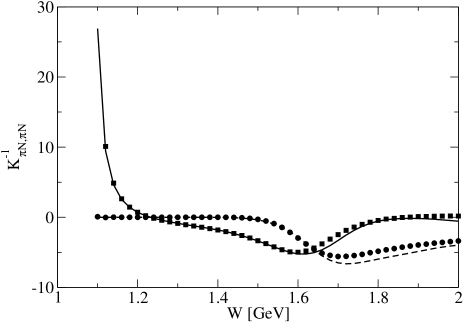
Figure 2: The inverse Heitler $K$ matrix element $K^{-1}_{\pi N,\pi N}$ as function of the center-of-mass energy, $W$ calculated using Eq.(22). The dynamical model elements of Ref.Paris (2009) are shown as continuous curves: solid (dashed) curves show the real (imaginary) part. The SP06 solution of Ref.Arndt et al. (2006), which are very similar to the dynamical model curves, are indicated by squares (circles) for the real (imaginary) parts. The imaginary part, which should strictly be zero by unitarity, deviates from zero above $W\approx 1.45$ GeV since we have inverted the matrix element by ignoring inelastic effects. The pole position of the Heitler $K$ matrix, Eq.(16) may be read off the figure at the node of $K^{-1}_{\pi N,\pi N}$.

Verification of the Heitler $K$ matrix pole positions in the dynamical model and CM parametrization may be carried out graphically, as shown in Fig.(2). We may obtain the inverse of the $\pi N\to\pi N$ $K$-matrix element directly from the on-shell $\pi N\to\pi N$ $T$-matrix element calculated in the dynamical model approximately as

$$K_{\pi N,\pi N}^{-1} \approx i+T_{\pi N,\pi N}^{-1}.$$ (22)

for values of $W$ above the $\pi N$ threshold. Here we have absorbed the factor $\rho$ from Eq.(10) by a redefinition of $K$ and $T$. The zero of the inverse Heitler $K$-matrix element, $K_{\pi N,\pi N}$ is the location of the matrix element’s pole. The derivation of Eq.(22) has neglected the other, inelastic channels. The neglect of other channels, present in both the dynamical model of Ref.Paris (2009), which includes $\pi\Delta,\rho N,\sigma N,$ and $\eta N$ and the SAID SP06 parametrization, which includes $\pi\Delta,\rho N,$ and $\eta N$ is warranted, as shown in Fig.(2). In this figure, violations of unitarity incurred by ignoring the inelastic processes appear as the imaginary part of $K^{-1}_{\pi N,\pi N}$ deviates from zero, above about 1.45 GeV according to the figure, where Eq.(22) is no longer valid. The location of the pole in the Heitler $K$ matrix can be read directly off the figure. The numerical value of $1.23$ GeV is the same as that of the SAID parametrization given in Eq.(16).

III Conclusion

The dynamical coupled-channels approach has been compared with the CM parametrization for the $P_{33}$ partial wave. The SAID parametrization, specifically the SP06 solution of Ref.Arndt et al. (2006), includes an explicit pole in the CM $K$ matrix, $\overline{K}$, as given in Eq.(13). The relationship between the CM $K$ matrix and the Heitler $K$ matrix, $K$, depicted in Eq.(1), demonstrates that the ‘bare’ CM pole is dressed by off-shell effects, represented by the real part of the CM diagonal matrix, $\mbox{Re }\!C(W)$. The Heitler $K$ matrix pole is further dressed by the coupling to intermediate states in the continuum, through the effects encoded in the relationship between the $K$ matrix and the $T$ matrix of Eq.(10).

Numerically, the description of the pole structure of $\overline{K}$, $K$, and $T$ bear a strong relationship to that of the dynamical model of Refs.Julia-Diaz et al. (2007) and Paris (2009). In these models, the bare pole of the interaction kernel, $V$ is related to the poles of the $K$ matrix by Eq.(21). The second term of this relation gives the rescattering effects of the off-shell intermediate states, in close parallel to the form of Eqs.(1) or (11). Having established the numerical identity of the Heitler $K$ matrix poles, the fact that the dynamical model is fit to the $\pi N$ elastic partial waves amplitudesJulia-Diaz et al. (2007) one is guaranteed that the $T$ matrix poles are virtually identical in both the parametrization and model approaches.

The numerical identity of the pole structure of these two ostensibly different approaches suggests a connection between them at the dynamical level. The loop dynamics of the rescattering effects, explicit in the microscopic, model dependent formulation of the dynamical coupled channels approach is a fundamental aspect of hadronic reactions and is believed to play a key role in the understanding of single and multiple meson reactions. It is encouraging that the CM approach, which gives model independentWorkman and Paris (2010) parametrizations of the $\pi N$ elastic partial wave amplitudes, encodes the dynamics of the model approach.

Finally, we emphasize in closing, that the specific value of the bare pole in the dynamical model, $M^{(0)}(P_{33})=1391$ MeV is a model dependent quantity. The value of this bare parameter, which appears in the Lagrangian, depends on several factors including the assumed unstable particle content (the assumed channel space), regularization (ie., form factors) and approximations. In fact, the well developed coupled-channel dynamical Jülich model gives a different value for the bare mass. Reference Gasparyan et al. (2003) gives, in their Table (5.3), the value 1459 MeV. Indeed, model dependence can even be seen within a given approach, if different model spaces and approximations are considered. As examples of this, we can look at the dynamical coupled-channel model of Ref.Sato and Lee (1996), a precursor of the models in Refs.Julia-Diaz et al. (2007) and Paris (2009). Table I of Ref.Sato and Lee (1996) gives $M^{(0)}(P_{33})$ (their $m_{\Delta}$) as 1299 (1319) MeV for model L(H). Alternatively, we observe various values of the bare mass in different versions of the Jülich model. Table I from Ref.Schütz et al. (1994) we see the value 1375 MeV, which can be compared to the value 1459 MeV quoted from Ref.Gasparyan et al. (2003) above. The origin of these shifts in the bare pole mass are identifiable as a consequence of the particular details of a given model formulation. The shifts do not indicate, at least to us, a measure of the quality of any given model. Nevertheless, the model dependence of the bare parameters are seen clearly and our earlier caveat appears warranted. Here, however, we have made the case that despite the model dependence of the bare pole position, certain features of dynamical model treatements and our CM parametrization approach are similar insofar as their dynamical treatment is quantitatively comparable.