Atomic matter-wave revivals with definite atom number in an optical lattice

Abstract

We study the collapse and revival of interference patterns in the momentum distribution of atoms in optical lattices, using a projection technique to properly account for the fixed total number of atoms in the system. We consider the common experimental situation in which weakly interacting bosons are loaded into a shallow lattice, which is suddenly made deep. The collapse and revival of peaks in the momentum distribution is then driven by interactions in a lattice with essentially no tunnelling. The projection technique allows to us to treat inhomogeneous (trapped) systems exactly in the case that non-interacting bosons are loaded into the system initially, and we use time-dependent density matrix renormalization group techniques to study the system in the case of finite tunnelling in the lattice and finite initial interactions. For systems of more than a few sites and particles, we find good agreement with results calculated via a naive approach, in which the state at each lattice site is described by a coherent state in the particle occupation number. However, for systems on the order of 10 lattice sites, we find experimentally measurable discrepancies to the results predicted by this standard approach.

I Introduction

In the early days of Bose Einstein condensates (BECs) with atomic gases there was a lively debate how to reconcile the notion of the phase of a BEC with atom number conservation Leggett:1991 ; leggettbook ; Javanainen:1996 . In condensed matter physics this discussion goes back to Leggett’s work of spontaneously broken gauge symmetries, and the observability and meaning of an absolute phase of a condensate, and of a relative phase between two BECs Leggett:1991 ; leggettbook . An absolute condensate phase – provided we understand the BEC order parameter $\langle\hat{\psi}(\mathbf{x},t)\rangle$ as expectation value of the boson particle destruction operator – implies a coherent superposition of states of atom numbers as in a coherent state. However, in a theory where all observables commute with the number operator, the phase of such superpositions remains unobservable on a fundamental level. On the other hand, the relative phase of two condensates, associated with superposition states of atom number differences between two BECs, is consistent with particle number conservation, and is observable in an interference experiment which measures a correlation function $\langle\hat{\psi}^{{\dagger}}(\mathbf{x},t)\hat{\psi}(\mathbf{x}^{\prime},t^{\prime})\rangle$ Andrews:1997 . As in the case of coherence of light in quantum optics qfcGZ , the factorization property of the correlation function $\langle\hat{\psi}^{{\dagger}}(\mathbf{x},t)\hat{\psi}(\mathbf{x}^{\prime},t^{\prime})\rangle\rightarrow\psi^{\ast}(\mathbf{x},t)\psi(\mathbf{x}^{\prime},t^{\prime})$ for a given quantum state implies full visibility of the interference pattern, and provides a measurement of the BEC order parameter in a number conserving context. The emergence of interference fringes in a quantum measurement process based on successive detection of atoms for two BECs prepared initially in a product of Fock states (eigenstates of fixed particle number) was analyzed in a language and formalism familiar from photon detection in quantum optics in Refs. Javanainen:1996 . Detection of an atom in an interference experiment erases the “which path” information from which BEC the atom came from, and thus prepares a superposition state of atom number differences compatible with number conservation.

Collapse and revival dynamics due to interactions in a BEC loaded into an optical lattice, as described by a Hubbard model and observed in the visibility of interference fringes after releasing atoms from the trap Greiner02 ; Will10 , is a second example where traditionally atomic number superpositions in the form of coherent states are invoked in the theoretical derivation and interpretation Wright96 ; Imamoglu97 ; Milburn97 ; Walls97 . Somewhat surprisingly, a derivation of this phenomenon in a discussion respecting number conservation seems to be missing in the literature. Below we will provide analytical collapse and revival formulas for finite particle number, where we see the emergence of the usual results in the limit of an infinite number of wells. On the more practical side, we will also connect the collapse and revival signal with a number conserving time-dependent DMRG treatment of Bose-Hubbard dynamics in a 1D optical lattice. This makes it possible to calculate systematically corrections due to finite tunneling between the wells and finite initial interactions which has not been possible in previous work.

Collapse and revival of interference patterns driven by two-body interactions was first raised in discussing the dynamics of Bose-Einstein Condensates (BECs) in a double well Milburn97 ; Walls97 , and later was investigated with cold atoms in optical lattices Greiner02 ; Will10 . In these lattice experiments, weakly interacting bosons are typically loaded into a shallow lattice, which is then suddenly made deep. This prevents tunnelling of atoms between neighbouring sites, and the interference pattern corresponding to the momentum or quasi-momentum distribution of atoms in the lattice undergoes collapses and revivals due to on-site interactions. Most recently, these dynamics were used to investigate the dependence of on-site interaction energy shifts on the occupation number of a lattice site in a 3D optical lattice Will10 ; Johnson09 . Dynamics of collapses and revivals driven by two-body interactions have also been studied in the context of hard-core bosons superlattice Rigol06 , Bloch oscillations in a tilted lattice Kolovsky03 ; Kolovsky09 , and double well superlattice experiments, Anderlini06 ; Sebby-Strabley07 .

In essentially all of these cases, the experiments have been described based on an ansatz in which the initial state of the non-interacting BEC can naively be represented as a product of local coherent states in the onsite occupation number. This can be represented as

$$|\mathrm{BEC}_{\mathrm{naive}}\rangle=\prod_{i}^{M}e^{-\frac{|\beta_{i}|^{2}}{2}}e^{\beta_{i}b_{i}^{\dagger}}|\mathrm{vac}\rangle,$$ (1)

where, $b_{i}^{\dagger}$ denotes the creation operator for particles on site $i$, and $|\beta_{i}|^{2}$ is the local mean particle number. As we show below, this ansatz reduces to the correct non-interacting ground state in an infinite system, but in a finite-size system does not have a fixed total number of particles.

In a deep lattice, the time-evolution of this state is simply governed by two-body onsite interactions generated by the Hamiltonian term $(U/2)\sum_{i}^{M}\hat{n}_{i}(\hat{n}_{i}-1)$, with the number operator $\hat{n}_{i}=b_{i}^{\dagger}b_{i}$. We find that expectation values such as the single-particle density matrix (SPDM) factorize, so that for a homogeneous system, we obtain ($\hbar\equiv 1$):

$$\langle b_{i}^{{\dagger}}b_{j}\rangle_{t} =\langle b_{i}\rangle_{t}^{*}\langle b_{j}\rangle_{t}$$

$$=\beta_{i}^{*}\beta_{j}e^{|\beta_{i}|^{2}(e^{iUt}-1)}e^{|\beta_{j}|^{2}(e^{-iUt}-1)}$$ (2)

$$=|\beta|^{2}e^{|\beta|^{2}(2\cos(Ut)-2)},$$ (3)

with $\beta_{i}=\beta$ in the homogeneous system.

This naive number non-conserving ansatz leads to wrong results for small particle numbers, which could be quantitatively measured in an experiment. In this paper, we demonstrate this by calculating the exact results for finite systems and a fixed total number of particles via a projection operator approach. At the same time, we confirm that the naive ansatz yields accurate results, even for suprisingly moderate-sized systems larger than about five particles on five lattice sites.

The approach we use here is similar to that used in previous studies of Bose-Einstein condensates, where a Fock state of fixed particle number is written as a phase averaged coherent state Javanainen:1996 . Our results for a finite system are in agreement with previous work for homogeneous systems based on a binomial expansion (see Ref. bach2004 ), and we are also able to treat systems with open boundary conditions and trapping potentials. Using an optimised version of the Time-Evolving Block Decimation algorithm (TEBD) Vidal03 ; Vidal04 , we also study and discuss the effects of finite tunnelling in the lattice during time evolution Fischer08 ; Wolf10 , as well as weak interactions in the initial state. Though for clarity we focus on results here in which the atoms are arranged along one dimension (e.g., with tight confinement in a 3D optical lattice), the results can be generalized straightforwardly to higher dimensions.

The rest of this paper is organized as follows: In Sec. II we first present the details of the system we study, including the Bose-Hubbard model, and the quasi-momentum distributions and correlation functions we calculate. In Sec. III we present exact results for revivals in this system, accounting properly for the conserved total number of particles in the system, and comparing the results to the naive approach outlined above. We account also for trapping potentials, finite tunneling in the lattice, and interactions in the initial state. In Sec. IV we present a summary and outlook for this work.

II The Model

We consider cold atoms loaded into the lowest Bloch band of an optical lattice Jak98 ; Blo08 ; Lew07 , which are described by the Bose-Hubbard Hamiltonian ($\hbar=1$)

$$H =-J(t)\sum_{\langle i,j\rangle}b_{i}^{{\dagger}}b_{j}+\frac{U(t)}{2}\sum_{i}\hat{n}_{i}(\hat{n}_{i}-1)+\sum_{i}\varepsilon_{i}b_{i}^{\dagger}b_{i},$$ (4)

where $b_{i}^{({\dagger})}$ are the bosonic annihilation (creation) operators at site $i$, $J$ denotes the tunneling amplitude between neighboring sites, $U$ denotes the onsite interaction energy shift for two atoms, $\hat{n}_{i}=b_{i}^{\dagger}b_{i}$ and $\varepsilon_{i}$ is the energy offset on different sites, which arises due to external trapping. We will assume that we have a total of $N$ particles on the $M$ lattice sites.

We assume that at time $t=0$, the system is loaded in the ground state of the Hamiltonian in a relatively shallow lattice where that atoms are weakly interacting. At time $t=0$ the depth of the lattice is rapidly increased, on a timescale that is fast compared with the tunneling time $\sim J^{-1}$, but slow compared with excitations to higher Bloch bands. In this way, the parameters $J$ and $U$ are changed suddenly at time $t=0$, so that

$$J(t)=\left\{\begin{array}[]{ll}J_{0},&\hbox{$t\leq 0$;}\\ J&\hbox{$t>0$.}\end{array}\right.,\>\>U(t)=\left\{\begin{array}[]{ll}U_{0},&\hbox{$t\leq 0$;}\\ U&\hbox{$t>0$.}\end{array}\right..$$ (5)

Below we will first analyze the ideal case, of an initial non-interacting BEC, so that $U_{0}=0$, and we have $N$ particles all in the same single-particle ground state of the Bose-Hubbard model. For a single particle, the ground state in this system can be written as

$$|\varphi\rangle=\frac{1}{\sqrt{N}}\sum_{i}^{M}\beta_{i}\hat{b}_{i}^{\dagger}|\mathrm{vac}\rangle,$$ (6)

with complex amplitudes $\beta_{i}$ that are dependent on the external potential $\varepsilon_{i}$. Note that we normalize these amplitude to the particle number $N$, i.e. $\sum_{i}^{M}|\beta_{i}|^{2}=N$, for reasons which become clear below. Then, the initial state for $N$ particles reads

$$|\mathrm{BEC}_{N}\rangle=\frac{1}{\sqrt{N!N^{N}}}\left(\sum_{i}^{M}\beta_{i}\hat{b}_{i}^{\dagger}\right)^{N}|\mathrm{vac}\rangle.$$ (7)

In the ideal case, after increase of the lattice depth, the tunneling will be negligible on the timescales of interest after the lattice depth is increased, i.e., $J\approx 0$. Both of these ideal conditions will be relaxed in Sec. III.5.

As mentioned above, collapses and revivals as studied in the experiments are observed via modulation of the visibility of interference fringes in the density distribution of the atomic cloud after a free expansion (time-of-flight measurement). This effectively measures the quasi-momentum distribution $n_{q}(t)$ after a certain hold time in the lattice $t$, defined as:

$$n_{q}(t)\equiv\frac{1}{M}\sum_{i,j}^{M}\langle b_{i}^{{\dagger}}b_{j}\rangle_{t}e^{iq(x_{i}-x_{j})},$$ (8)

where $x_{i}$ are the discrete site-positions in the lattice, and $\langle b_{i}^{\dagger}b_{j}\rangle_{t}$ is the time-dependent single particle density matrix (SPDM). Note that so far we consider a system in arbitrary dimensions and with arbitrary lattice geometry. Thus, in general the $x_{i}$ and $q$ are vectors. Along a single dimension, we consider a lattice constant $a$, and the discrete positions in that dimension can be written as $x^{\mathrm{1D}}_{i}=ai$. Thus, along that dimension, which consists of $M^{\mathrm{1D}}$ sites, the quasi-momenta can have the discrete values $q^{\mathrm{1D}}=n2\pi/aM^{\mathrm{1D}}$ (with integer $n=1\dots M^{\mathrm{1D}}$). In the following we will focus on the calculation of the time-evolution of the SPDM elements.

III Exact results for Revivals in the Bose-Hubbard model

In this section, we present our results for revivals in the Bose-Hubbard model, correctly accounting for the fixed total number of particles in the system. We begin with a simple example of where the naive treatment breaks down, by studying two particles on two lattice sites in Sec. III.1. In Sec. III.2 we then provide technical details of the projection method used to derive exact results in the case that atoms are initially non-interacting ($U_{0}=0$) and that tunneling in the deep lattice is negligible ($J=0$). The exact results for these cases are then summarized and compared with the naive approach for homogeneous systems in Sec. III.3 and for inhomogeneous systems in Sec. III.4. In Sec. III.5 we will relax these conditions ($U_{0}=J=0$), accounting for finite tunnelling and finite interactions in the initial state by performing essentially exact many-body numerical computations.

III.1 Two particles on two lattice sites

We begin with a simple example for which the ansatz of on-site coherent states, Eq. (1) clearly gives the wrong results. This can be easily demonstrated for two particles on two lattice sites ($N=M=2$) without external trapping, for which the initial state will be given by $|\mathrm{\psi_{2}}\rangle_{0}=(|02\rangle+|20\rangle)/2+|11\rangle/\sqrt{2}$, where $|n_{1}n_{2}\rangle$ denotes a state with $n_{1}$ particles on the first site and $n_{2}$ particles on the second site. Time-evolving this state under the Hamiltonian (4) gives

$$|\mathrm{\psi_{2}}\rangle_{t}=\frac{1}{2}\left(e^{-iUt}|02\rangle+e^{-iUt}|20\rangle\right)+\frac{1}{\sqrt{2}}|11\rangle,$$ (9)

so that the off-diagonal SPDM elements in a two-site system with two particles are given by

$$\langle b_{1}^{\dagger}b_{2}\rangle=\langle b_{2}^{\dagger}b_{1}\rangle=\cos{(Ut)}.$$ (10)

This clearly contradicts the result from Eq. (3), as can be seen in Fig. 1.

III.2 Particle number projection method

In order to conveniently calculate the time evolution for an arbitrary number of particles, we now introduce an operator $P_{N}$, which projects states onto a subspace of the Hilbert space with fixed total particle number $N$. The operator $P_{N}$ itself does not preserve the normalization of a state and thus requires an additional renormalization factor $\mathcal{N}$. With this operator, we can show that any state of the form (7) can be written as a projection of the coherent product state

$$|\{\beta_{k}\}\rangle \equiv\prod_{k}^{M}|\beta_{k}\rangle_{k}\equiv\prod_{k}^{M}e^{-\frac{|\beta_{k}|^{2}}{2}}e^{\beta_{k}b_{k}^{{\dagger}}}|\mathrm{vac}\rangle.$$ (11)

The number projection of this state reads

$$P_{N}|\{\beta_{k}\}\rangle =e^{-\frac{1}{2}\sum_{k}^{M}|\beta_{k}|^{2}}P_{N}e^{\sum_{k}^{M}\beta_{k}b_{k}^{{\dagger}}}|\mathrm{vac}\rangle$$

$$=e^{-\frac{1}{2}\sum_{k}^{M}|\beta_{k}|^{2}}P_{N}\sum_{n=0}^{\infty}\frac{1}{n!}\left(\sum_{k}^{M}\beta_{k}b_{k}^{\dagger}\right)^{n}|\mathrm{vac}\rangle$$

$$=\frac{1}{\sqrt{\mathcal{N}}}e^{-\frac{1}{2}\sum_{k}^{M}|\beta_{k}|^{2}}\frac{1}{N!}\left(\sum_{k}^{M}\beta_{k}b_{k}^{\dagger}\right)^{N}|\mathrm{vac}\rangle.$$ (12)

This coincides with the general inital many-body ground state (7) with the normalization factor $\mathcal{N}=e^{-N}N^{N}/N!$, which has the form of a Poisson distribution in the total particle number $N$. Note that we used $\sum_{k}^{M}|\beta_{k}|^{2}=N$.

To perform calculations conveniently we can write the projection operator in the form of a phase integral

$$P_{N} =\frac{1}{2\pi\sqrt{\mathcal{N}}}\int_{-\pi}^{\pi}d\phi\,e^{i(\hat{N}-N)\phi},$$ (13)

with the total particle number operator $\hat{N}=\sum_{i}b_{i}^{\dagger}b_{i}$. Note that the projection operator $P_{N}$ has the properties $\mathopen{[}P_{N},b_{i}^{\dagger}b_{j}\mathclose{]}=\mathopen{[}P_{N},H\mathclose{]}=0$ for all $i$, $j$, and $P_{N}^{2}=P_{N}/\sqrt{\mathcal{N}}$.

The benefit of writing the BEC ground state as number projection of the $|\{\beta_{k}\}\rangle$ state, with the projector from Eq. (13) is that the SPDM then factorizes with additional phase integrals that can be solved exactly. We consider the time-evolved SPDM under the evolution of Hamiltonian (4), which is given by

$$\langle b_{i}^{{\dagger}}b_{j}\rangle_{t} =\langle\mathrm{BEC}_{N}|e^{iHt}b_{i}^{{\dagger}}b_{j}e^{-iHt}|\mathrm{BEC}_{N}\rangle$$

$$=\frac{1}{2\pi\mathcal{N}}\int_{-\pi}^{+\pi}d\phi\,e^{-iN\phi}$$

$$\qquad\times\langle\{\beta_{k}\}|e^{iHt}b_{i}^{{\dagger}}b_{j}e^{-iHt}e^{\hat{N}\phi}|\{\beta_{k}\}\rangle$$

$$=\frac{1}{2\pi\mathcal{N}}\int_{-\pi}^{+\pi}d\phi\,e^{-iN\phi}$$

$$\qquad\times\langle\{\beta_{k}\}|e^{iHt}b_{i}^{{\dagger}}b_{j}e^{-iHt}|\{\beta_{k}e^{i\phi}\}\rangle.$$ (14)

In the last line we have used the fact that

$$e^{i\phi b_{k}^{\dagger}b_{k}}|\beta_{k}\rangle_{k}=\sum_{n=0}^{\infty}\frac{\beta_{k}^{n}}{\sqrt{n!}}e^{i\phi n}|n\rangle_{k}=|\beta_{k}e^{i\phi}\rangle_{k}$$ (15)

for every site $k$.

We can then exactly evaluate the SPDM elements from Eq. (14) for time-evolution under the Hamiltonian (4). In the diagonal case, $\mathopen{[}H,b_{i}^{\dagger}b_{i}\mathclose{]}=0$, and thus the diagonal elements are time-invariant. At $t=0$, we find

$$\langle b_{i}^{{\dagger}}b_{j}\rangle_{t=0} =\frac{\beta_{i}^{*}\beta_{j}}{2\pi\mathcal{N}}\int_{-\pi}^{\pi}d\phi\,e^{-i(N-1)\phi}e^{\sum_{k}^{M}|\beta_{k}|^{2}(e^{i\phi}-1)},$$ (16)

where we used $b_{k}|\beta_{k}\rangle_{k}=\beta_{k}|\beta_{k}\rangle_{k}$, and $\langle\alpha^{*}|\beta\rangle=e^{\alpha^{*}\beta-|\alpha|^{2}/2-|\beta|^{2}/2}$. Integrals of the form of Eq. (16) can be solved with the parametrization $z=e^{i\phi}$. This yields

$$\langle b_{i}^{{\dagger}}b_{j}\rangle_{t=0} =\frac{\beta_{i}^{*}\beta_{j}}{2\pi i\mathcal{N}}e^{-N}\oint_{\mathcal{C}}dz\,\frac{1}{z^{N}}e^{Nz}$$

$$=\frac{\beta_{i}^{*}\beta_{j}}{\mathcal{N}}e^{-N}\frac{1}{(N-1)!}\lim_{z\to 0}\left[\frac{\partial^{N-1}}{\partial z^{N-1}}e^{Nz}\right]$$

$$=\beta_{i}^{*}\beta_{j},$$ (17)

where the integration takes place along the complex unit circle, denoted by $\mathcal{C}$, and we again used $\sum_{k}|\beta_{k}|^{2}=N$. Thus, the initial SPDM factorizes into $\beta_{i}^{*}\beta_{j}$, and the diagonal elements remain constant in time $\langle b_{i}^{{\dagger}}b_{i}\rangle_{t}=|\beta_{i}|^{2}$.

We finally calculate the time-evolution of the off-diagonal SPDM elements. We write the Hamiltonian (4) as $H\equiv\sum_{i}^{M}h_{i}$ and find for $i\neq j$

$$\langle\{\beta_{k}\}|e^{iHt}b_{i}^{{\dagger}}b_{j}e^{-iHt}|\{\beta_{k}e^{i\phi}\}\rangle$$

$$\quad=\langle\beta_{i}|e^{ih_{i}t}b_{i}^{{\dagger}}e^{-ih_{i}t}|\beta_{i}e^{i\phi}\rangle_{i}\langle\beta_{j}|e^{ih_{j}t}b_{j}e^{-ih_{j}t}|\beta_{j}e^{i\phi}\rangle_{j}$$

$$\qquad\times\prod_{k\neq i,j}\langle\beta_{k}|\beta_{k}e^{i\phi}\rangle_{k}.$$ (18)

The factorized elements can be straightforwardly calculated as

$$\langle\beta_{j}|e^{ih_{j}t}b_{j}e^{-ih_{j}t}|\beta_{j}e^{i\phi}\rangle_{j}=\beta_{j}e^{i\phi}e^{-i\varepsilon_{j}t}e^{|\beta_{j}|^{2}\left[e^{i\phi}e^{-iUt}-1\right]},$$ (19)

and

$$\langle\beta_{i}|e^{ih_{i}t}b_{i}^{\dagger}e^{-ih_{i}t}|\beta_{i}e^{i\phi}\rangle_{i}=\beta_{i}^{*}e^{i\varepsilon_{i}t}e^{|\beta_{i}|^{2}\left[e^{i\phi}e^{iUt}-1\right]}.$$ (20)

In total we find ($i\neq j$):

$$\langle b_{i}^{{\dagger}}b_{j}\rangle_{t} =\frac{\beta_{i}^{*}\beta_{j}}{2\pi\mathcal{N}}\,e^{-N}e^{i(\varepsilon_{i}-\varepsilon_{j})t}\int_{-\pi}^{+\pi}d\phi\,e^{-i(N-1)\phi})$$ (21)

$$\quad\times e^{e^{i\phi}\left[|\beta_{j}|^{2}e^{-iUt}+|\beta_{i}|^{2}e^{iUt}+\sum_{k\neq i,j}|\beta_{k}|^{2}\right]}$$

$$=\beta_{i}^{*}\beta_{j}e^{i(\varepsilon_{i}-\varepsilon_{j})t}$$

$$\times\left[\frac{1}{N}\left(|\beta_{j}|^{2}e^{-iUt}+|\beta_{i}|^{2}e^{iUt}+\sum_{k\neq i,j}|\beta_{k}|^{2}\right)\right]^{(N-1)},$$

where we again used the parametrization $z=e^{i\phi}$ and an integration along a complex unit circle.

III.3 Revivals in a homogeneous system (periodic boundary conditions)

In the case of a homogeneous density, $\beta_{i}=\beta=\sqrt{N/M}$ for all $i$. This implies that we assume periodic boundary conditions, and no external trapping ($\varepsilon_{i}=0$ for all $i$). The off-diagonal SPDM elements then become site-independent, with Eq. (21) simplifying to

$$\langle b_{i}^{{\dagger}}b_{j}\rangle_{t} =|\beta|^{2}\left[1+\frac{|\beta|^{2}}{N}\left(2\cos{(Ut)}-2\right)\right]^{(N-1)}.$$ (22)

For $N=M=2$, we reproduce the exact result from Eq. (10). In the limit where the particle number is much larger than the onsite density, i.e., $N\gg|\beta|^{2}$, we find

$$|\beta|^{2}\left[1+\frac{|\beta|^{2}}{N}\left(2\cos(Ut)-2\right)\right]^{(N-1)}$$

$$\overset{N\gg|\beta|^{2}}{\longrightarrow}|\beta|^{2}e^{|\beta|^{2}\left[2\cos(Ut)-2\right]},$$ (23)

since $\lim_{N\to\infty}(1+x/N)^{N}=e^{x}$. Hence, in this limit we reproduce exactly the result of the naive treatment from Eq. (3).

For homogeneous densities, the height of the $q=0$ peak in the quasi-momentum distribution is given by $n_{q=0}=(1/M)\sum_{i,j}^{M}\langle b_{i}^{{\dagger}}b_{j}\rangle_{t}=(M-1)\langle b_{i}^{{\dagger}}b_{j}\rangle+|\beta|^{2}$. Thus, the experimentally measured visibility of time-of-flight interference fringes is directly connected to the site-independent off-diagonal SPDM elements. In Fig. 1 we show a plot of the time-evolution of the these elements beginning from an ideal non-interacting ground state with density $|\beta|^{2}=1$, and including the first collapse and revival. For increasing particle numbers, we see that the results from Eq. (22) converge rapidly to the values given by the naive treatment in Eq. (3). Indeed, already for moderate numbers, $N\sim 5$, the exact results are very close to the approximate result.

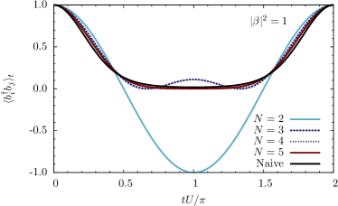
Figure 1: Plot of the time-evolution of the off-diagonal SPDM elements for an initial ideal superfluid state ($U_{0}=0$) with homogeneous density and without external trapping ($\varepsilon_{i}=0$) in a deep optical lattice ($J=0$). The density is chosen as one particle per site ($|\beta|^{2}=1$), and we show the first collapse and revival for increasing number of particles. We compare results from the exact treatment of Eq. (22) to the naive result from Eq. (3) (solid black line). Periodic boundary conditions are assumed.

We can define the relative error in the visibility of interference fringes, i.e. the relative error in the height of the $n_{q=0}$ peak between the naive and the exact treatment as

$$\epsilon_{t}\equiv\frac{n_{q=0}^{\mathrm{exact}}-n_{q=0}^{\mathrm{naive}}}{n_{q=0}^{\mathrm{exact}}},$$ (24)

where $n_{q=0}^{\mathrm{exact}}$ is obtained from Eq. (22) and $n_{q=0}^{\mathrm{naive}}$ from Eq. (3). Using the parametrization $\alpha_{t}\equiv|\beta|^{2}(2\cos(Ut)-2)$, i.e. $-4|\beta|^{2}\leq\alpha_{t}\leq 0$, and expanding in powers of $1/N$, we find

$$\epsilon_{t}=-\frac{2\alpha_{t}+\alpha_{t}^{2}}{2N}-\frac{4\alpha_{t}^{3}+3\alpha_{t}^{4}}{24N^{2}}+\mathcal{O}\left({\frac{1}{N^{3}}}\right).$$ (25)

Thus, for large $N$ and small homogeneous densities, the relative error from the naive treatment decreases proportional to $1/N$. Note that this error can also be written in terms of the system size $M$. Up to first order we find for small densities $|\beta|^{2}$

$$\epsilon_{t}=-\frac{2\cos(Ut)-2}{M}-\frac{|\beta|^{2}(2\cos(Ut)-2)^{2}}{2M}+\mathcal{O}\left({\frac{1}{M^{2}}}\right).$$

The error decreases proportional to $1/M$. In the next section we will also treat the more general case of inhomogeneous densities below.

III.4 Revivals for inhomogeneous systems

Inhomogeneous densities arise from external trapping potentials, i.e. from site varying energy-offsets $\varepsilon_{i}$ in Eq. (4), or from confinement represented by open boundary conditions. The initial state for non-interacting particles on the lattice can be found by solving the single particle problem for the amplitudes $\beta_{i}$. Here we will focus on a 1D lattice array with $M$ sites, for which the initial single-particle Hamiltonian reads

$$H_{t<0} =-J_{0}\sum_{n}(|n\rangle\langle n+1|+\mathrm{h.c.})+\sum_{n}\epsilon_{n}|n\rangle\langle n|,$$ (26)

where $|n\rangle$ denotes the state for a particle being at site $n$. Without external trapping ($\epsilon_{n}=0$ for all $n$) and for periodic boundary conditions ($|M+1\rangle\equiv|1\rangle$), the eigenstates of Hamiltonian (26) are simply given by $|\varphi_{m}\rangle=\sum_{j=1}^{M}\exp(iq_{m}aj)|j\rangle/\sqrt{M}$, with quasi-momenta $q_{m}=2\pi m/aM$ and eigenenergies $E_{m}=-2\cos(q_{m}a)$.

For the case of box boundary conditions, we can write the system on a grid of $M+2$ sites (labeled by $i=0,\dots,M+1$), and local energy offsets $\epsilon_{0},\epsilon_{M+1}\rightarrow\infty$, and $\epsilon_{n\neq 0,M+2}=0$. To fulfill the boundary conditions, the eigenstates are then given by $|\varphi_{m}\rangle=\sum_{j=0}^{M+1}\sin(q_{m}aj)|j\rangle/\sqrt{\mathcal{M}}$ with normalization $\mathcal{M}\equiv\sum_{j=0}^{M+1}\sin^{2}(q_{m}aj)$. The quasi-momenta are given by $q_{m}=m\pi/(M+1)a$, where $m>0$, and the eigenenergies are $E_{m}=-2\cos(q_{m}a)$. Thus, the coefficients $\beta_{i}$ for the renormalized single-particle ground-state (6) are given by

$$\beta_{i}=\sqrt{\frac{N}{\mathcal{M}}}\sin\left(\frac{\pi}{M+1}i\right)$$ (27)

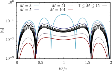
Figure 2: The time-evolution of the relative error $\epsilon_{t}$ of the naive approach compared with exact results in the height of the quasi-momentum distribution peak (i.e. $n_{q=0}$). The results are for a 1D system with box boundary conditions, resulting in a site-dependent particle density. Results are shown for the time-evolution of the error until the first revival at $t=2\pi/U$, and for increasing system sizes ($N=M$, $U_{0}=0$, $J=0$, $\varepsilon_{i}=0$).

In Fig. 2, we plot the relative error $\epsilon_{t}$ between the exact and the naive treatment when we begin from an inhomogeneous initial state due to box boundary conditions. We show the time-evolution of the error in the height of the $q=0$ quasi-momentum peak, as defined in Eq. (24), covering the time-scale of the first collapse and revival until $t=2\pi/U$ in a system with $N=M$ particles. We find that $\epsilon_{t}$ generally decreases with increasing system size, and assumes its largest value approximately in the middle of the collapse process at $t\approx\pi/4U$.

To analyze the scaling of the error in the particle number $N$, in Fig. 3, we plot the relative error in the height of the $q=0$ quasi-momentum peak as a function of $N$. For homogeneous densities in the limit of large $N$, $\epsilon_{t}$ is given by Eq. (25), i.e. it decays proportional to $1/N$.

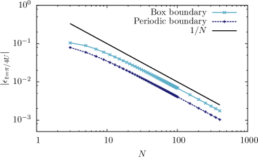
Figure 3: The scaling of the relative error $\epsilon_{t=\pi/4U}$ of the naive approach compared with the exact results at the middle of the first collapse $t=\pi/4U$. Results are shown both for periodic and open (box) boundary conditions. To compare the results to Eq. (25), we also plot $1/N$ ($U_{0}=0$, $J=0$, $\varepsilon_{i}=0$).

We thus find that for large $N$, the error scales as $1/N$ for both homogeneous and inhomogeneous densities studied here. For typical 1D lattice sizes in experiments of approximately $50$ sites, the relative error becomes of the order of $1\%$. In this sense, the naive treatment provides a good semi-quantitative description of the system. However, because experimental system sizes are of the order of 10–100 lattice sites, it should be possible to measure the quantitative discrepancies arising in the revivals as a result of finite system sizes and fixed particle numbers.

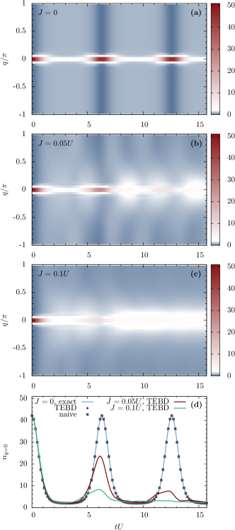
Figure 4: Time-evolution of the quasi-momentum distribution $n_{q}$ for several tunneling amplitudes $J$ in a system with $M=51$ sites and box boundary conditions. Initially the system is in the exact ground state for $U_{0}/J_{0}=0$. Panels (a)-(c) show exact results obtained numerically by using the TEBD algorithm. Panel (d) shows the evolution of the $n_{q=0}$ peak. The TEBD results for $J=0$ are compared to the exact results obtained from Eq. (21), and to the naive treatment obtained from Eq. (I). The particles are intitially non-interacting ($U_{0}=0$).

III.5 Effects of finite tunnelling or initial interactions

In this section we compare our results to numerical calculations for the 1D Bose-Hubbard model, in order to account for the effects of a non-zero tunneling amplitude $J$ during the time-evolution, and a non-zero initial interaction strength $U_{0}$. We consider the time-evolution of the quasi-momentum-distribution in systems up to $M=51$ sites, using the TEBD algorithm Vidal03 ; Vidal04 . This algorithm makes possible the near-exact integration of the Schrödinger equation for 1D lattice and spin Hamiltonians based on a matrix product state ansatz. We optimize the algorithm for fixed total particle numbers as is done in Density Matrix Renormalization Group methods dmrgrev ; tdmrg1 ; tdmrg2 ; tebdcons

In Fig. 4 we show results for the time evolution of the quasi-momentum distribution. We start with the exact ground state for box boundary conditions. It is obtained by an imaginary TEBD time-evolution and yields an initial density profile, $\beta_{i}$, consistent with Eq. (27). The exact time-evolution calculation covers the first two revivals within the time $0\leq tU\leq 5\pi\approx 15.7$. In panels (a)-(c) we show TEBD results for $J=0$, $J=0.05U$, and $J=0.1U$, respectively. In panel (d) we show the time-evolution of the peak of the quasi-momentum distribution, i.e. $n_{q=0}$. There, we compare the results from our TEBD calculations with the exact calculations for $J=0$, i.e. from Eq. (21), and the naive treatment from Eq. (I). For our numerical calculation, convergence in several numerical parameters had to be checked. For the results obtained in this section we have tested convergence of the TEBD algorithm for numerical parameters, and use matrix sizes up to $\chi=200$ Vidal03 ; Vidal04 , and allow occupation numbers up to 14 particles per lattice site.

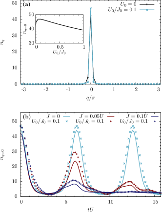
Figure 5: Panel (a) compares the initial quasi-momentum distribution for non-interacting particles ($U_{0}=0$) with the one for weakly interacting particles ($U_{0}/J_{0}=0.1$). Shown are results for a system with $51$ sites and box boundary conditions. The inset shows the scaling of the $n_{q=0}$ peak as a function of $U_{0}$. Panel (b) shows a comparison of the time-evolution of the $n_{q=0}$ peak for initially non interacting particles (solid-lines) with weakly interactings ones ($U_{0}/J_{0}=0.1$).

For $J=0$ results from the analytical number projection method (Eq. (21)) perfectly coincide with the TEBD results as expected, whereas visible differences are observed to the results from the naive treatment. These errors are small and scale as in Fig. 3. For non-zero tunneling, we find that the revivals are strongly damped, i.e. the peak in the momentum distribution for $q=0$ is smaller, and the quasi-momentum distribution at the revival time is broadened compared to the initial one. In addition, we see that the point in time of the first and the second revival are markedly shifted towards earlier times for increasing tunneling strength $J$. Both effects that appear here in exact numerical calculations of an 1D systems have been recently calculated perturbatively Fischer08 , and for hard-core bosons as well as on a mean-field level in high dimensions Wolf10 .

For non-zero initial interaction strength $U_{0}>0$, we note that the initial quasi-momentum distribution is slightly modified. However, the basic structure of the revivals is unaffected for $U_{0}\ll J_{0}$. This is shown in Fig. 5 for a system of $M=51$ sites and box-boundary conditions. We find that due to boundary effects for $U_{0}\lesssim 0.1J_{0}$, the quasi-momentum distribution for finite $U_{0}$ becomes narrowed compared to the one for non-interacting particles (Fig. 5(a)). Further increasing the initial interaction strength leads to a depletion of the $q=0$ state and a broadening of the quasi-momentum distribution (see inset). In Fig. 5(b) we compare the time-evolution for initially non-interacting particles (solid lines) with the one for $U_{0}/J_{0}=0.1$. We show $n_{q=0}$ for tunneling amplitudes $J/U=0$, $0.05$, and $0.1$ during time-evolution. We find that the point in time of the first and the second revival is not altered significantly due to $U_{0}\neq 0$. However, we find that the structure of the peaks modifies and is smoothed for $J/U>0$.

IV Summary & Outlook

By using a number projection method, we have shown that exact results can be derived for the collapse and revival of the SPDM for atoms in an optical latittce. We properly account for a fixed total number of particles in the system, and are able to take into account the effects of external potentials. For large numbers of particles $N$, we find that the discrepancy to naive calculations, based on assuming a coherent state on each site in the particle number scales as $1/N$. For as few as 5 particles on 5 sites, this approach can provide a good semi-quantitative approximation. However, the discrepancies should be measureable in experiments. Effects of finite tunnelling in the lattice, which can be treated perturbatively Fischer08 , or exactly for hard-core bosons Wolf10 can be investigated directly via time-dependent numerical calculations.

The general technique we use here could be extended to the case in which the onsite interaction strength is dependent on the occupation number, as has been observed in recent experiments Will10 .

- (1) A. Leggett and F. Sols, Foundations of Physics 21, 353 (1991).
- (2) A. J. Leggett, Quantum Liquids: Bose Condensation and Cooper Pairing in Condensed-Matter Systems, Oxford University Press, Oxford (2006).
- (3) J. Javanainen and S. M. Yoo. Phys. Rev. Lett. 76, 161 (1996); J. I. Cirac, C. W. Gardiner, M. Naraschewski, and P. Zoller, Phys. Rev. A, 54, R3714 (1996); Y. Castin and J. Dalibard, Phys. Rev. A 55, 4330 (1997).
- (4) M. R. Andrews et al., Science 275, 637 (1997).
- (5) C. W. Gardiner and P. Zoller, Quantum Noise (Springer, Berlin, 2004), and references cited.
- (6) M. Greiner, O. Mandel, T. W. Hänsch, and I. Bloch, Nature 419, 51 (2002).
- (7) S. Will, T. Best, U. Schneider, L. Hackermüller, D-S. Lühmann, and I. Bloch, Nature 465, 197 (2010).
- (8) E. M. Wright, D. F. Walls, and J. C. Garrison, Phys. Rev. Lett. 77, 2158 (1996); E. M. Wright, T. Wong, M. J. Collett, S. M. Tan, and D. F. Walls. Phys. Rev. A 56, 591 (1997).
- (9) A. Imamoglu, M. Lewenstein, and L. You, Phys. Rev. Lett. 78, 2511 (1997).
- (10) G. J. Milburn, J. Corney, E. M. Wright, and D. F. Walls, Phys. Rev. A 55, 4318 (1997).
- (11) D. F. Walls, M. J. Collett, T. Wong, S. M. Tan, and E. M. Wright, Phil. Trans. R. Soc. A 355, 2393 (1997).
- (12) P. R. Johnson, E. Tiesinga, J. V. Porto, and C. J. Williams, New J. Phys. 11, 093022 (2009).
- (13) M. Rigol, A. Muramatsu, and M. Olshanii, Phys. Rev. A 74, 053616 (2006).
- (14) A. R. Kolovsky, Phys. Rev. Lett. 90, 213002 (2003)
- (15) A. R. Kolovsky, H. J. Korsch, and E. M. Graefe, Phys. Rev. A 80, 023617 (2009).
- (16) M. Anderlini, J. Sebby-Strabley, J. Kruse, J. V. Porto, and W. D. Phillips, J. Phys. B: At. Mol. Opt. Phys. 39 S199 (2006).
- (17) J. Sebby-Strabley, B. L. Brown, M. Anderlini, P. J. Lee, W. D. Phillips, J. V. Porto, and P. R. Johnson, Phys. Rev. Lett. 98, 200405 (2007).
- (18) R. Bach and K. Rzazweski, Phys. Rev. A 70, 063622 (2004).
- (19) G. Vidal, Phys. Rev. Lett. 91, 147902 (2003).
- (20) G. Vidal, Phys. Rev. Lett. 93, 040502 (2004).
- (21) U. R. Fischer and R. Schützhold, Phys. Rev. A 78, 061603(R) (2008).
- (22) F. A. Wolf, I. Hen, and M. Rigol, Phys. Rev. A 82, 043601 (2010).
- (23) D. Jaksch, C. Bruder, J. I. Cirac, C. W. Gardiner, and P. Zoller, Phys. Rev. Lett. 81, 3108 (1998).
- (24) M. Lewenstein, A. Sanpera, V. Ahufinger, B. Damski, A. Sen, and U. Sen, Adv. Phys. 56, 243 (2007).
- (25) I. Bloch, J. Dalibard, and W. Zwerger Rev. Mod. Phys. 80, 885 (2008).
- (26) F. Verstraete, V. Murg, and J. I. Cirac, Adv. Phys. 57, 143 (2008).
- (27) A. J. Daley, C. Kollath, U. Schollwöck, G. Vidal, J. Stat. Mech.: Theor. Exp. P04005 (2004).
- (28) S. R. White and A. E. Feiguin, Phys. Rev. Lett. 93 , 076401 (2004).
- (29) A. J. Daley, S. R. Clark, D. Jaksch, and P. Zoller, Phys. Rev. A. 72, 043618 (2005).