Dynamics of a driven spin coupled to an antiferromagnetic spin bath

Abstract

We study the behavior of the Rabi oscillations of a driven central spin (qubit) coupled to an antiferromagnetic spin bath (environment). It is found that the decoherence behavior of the central spin depends on the detuning, driving strength, the qubit-bath coupling and an important factor, associated with the number of the coupled atoms, the detailed lattice structure, and the temperature of the environment. If the detuning exists, the Rabi oscillations may show the behavior of collapses and revivals; however, if the detuning is zero, such a behavior will not appear. We investigate the weighted frequency distribution of the time evolution of the central spin inversion and give this phenomenon of collapses and revivals a reasonable explanation. We also discuss the decoherence and the pointer states of the qubit from the perspectives of the von Neumann entropy. It is found that the eigenstates of the qubit self-Hamiltonian emerge as the pointer states in the weak system-environment coupling limit.

1 Introduction

One of the most promising candidates for quantum computation is the implementation using spin systems as quantum bits (qubits) [1, 2, 3, 4, 5, 6, 7]. Combining with nanostructure technology, they have the potential advantage of being scalable to a large system. In particular, the spin in a quantum dot exhibits a relatively long coherence time compared with fast gate operation times. This makes it a good candidate for a quantum information carrier [8, 9, 10, 11]. However the influence of the environment, especially the spin environment, on a spin, which usually causes the decoherence of the spin, is inevitable. Typically, the material environment must be present in order to host the spin or to locally control the electric or magnetic fields experienced by the spin. Therefore the decoherence behavior of a central spin or several spins interacting with a spin bath has attracted much attention in recent years [12, 13, 14, 15, 16, 17, 18, 19, 20, 21, 22, 23, 24, 25].

The problem of a central spin coupled to an antiferromagnetic (AF) spin environment was investigated in Refs. [26, 27, 28]. In these investigations, a pure dephasing model in which the self-Hamiltonian of the undriven central spin commutes with the interaction Hamiltonian to the environment was considered. A similar problem of a spin-$\frac{1}{2}$ impurity embedded in an AF environment was studied in the context of quantum frustration of decoherence in Ref. [29]. There the impurity spin is coupled locally in real space to just one spin of the AF environment, in contrast to the central spin model [30, 31, 32, 33, 34, 35, 36, 37, 38, 39, 40, 41] where the central spin is coupled isotropically with equal strength to all the spins of the environment. In this paper, we consider a more general case of a central spin (qubit) driven by an external field and coupled to an AF spin bath (environment). To control the quantum states of a qubit, some types of time-dependent controllable manipulations , which can be electrical [42], optical [43], or magnetic [44], are desirable. Thus it is important and necessary to study the behavior of a qubit (central spin) or several qubits (spins) interacting with an environment (a spin bath) in the presence of a driving field [45, 46, 47, 48]. Recently, the coherent dynamics of a single central spin (a nitrogen-vacancy center) coupled to a bath of spins (nitrogen impurities) in diamond was studied experimentally [47]. To realize the manipulation of the central spin, the pulsed radio-frequency radiation was used. Under the control of a time-dependent magnetic field, Ref. [48] considered a central spin system coupled to a spin bath. The decay of Rabi oscillations and the loss of entanglement were discussed. However, the correlations between spins in the spin bath were neglected. Recent investigations indicated that the internal dynamics of the spin bath could be crucial to the decoherence of the central spin [12, 13, 14, 15, 16, 17, 18, 19, 20, 21, 22]. In our driven spin model, the interactions between constituent spins of the AF environment are taken into account.

The self-Hamiltonian of the central spin, after a transformation to a frame rotating with the frequency of the driving field, can be written in a form of $H_{S}=\varepsilon S_{0}^{z}+gS_{0}^{x}$ in the rotating wave approximation. Due to the additional driving term of $gS_{0}^{x}$ that provides energy into the system and does not commute with the interaction Hamiltonian that couples to the AF environment in our model, the dynamics of the central spin in this case is dramatically different from the undriven pure dephasing behaviors investigated in Refs. [26, 27]. It was shown in Ref. [17] that the form and the rate of Rabi oscillation decay are useful in experimentally determining the intrabath coupling strength for a broad class of solid-state systems [17]. This is also the case in our problem. After the use of the spin-wave approximation to deal with the AF environment, we employed an elegant mathematic technique to trace over the AF environmental degrees of freedom exactly to obtain the reduced density matrix of the driven spin. This enables us to study and describe the decay behaviors of the Rabi oscillations for different initial states and parameters of the central spin-AF environment model beyond the Markovian approximation and Born approximation (perturbation). With the reduced density matrix obtained nonperturbatively, we also investigate and discuss the decoherence and the pointer states of the central spin from the perspective of the von Neumann entropy. We find that the decoherence behavior of the central spin depends on the detuning, driving strength, the coupling between the central spin and the spin environment, and an important factor $\Omega$, associated with the number of the spins, the lattice structure and the temperature of the environment. If the detuning exists, the Rabi oscillations may show a behavior of collapses and revivals; however, if the detuning is zero, such a behavior will not appear. We investigate the weighted frequency distribution of the time evolution of the central spin inversion and give this phenomenon a reasonable explanation. The form and the rate of Rabi oscillation decay is useful in determining the intrabath coupling strength and other related properties of the qubit-environment system [17]. Although we concentrate on the central spin model, our study is applicable to similar models of a pseudo spin or a qubit coupled to an environment. For example, in the study of the decoherence behavior of a flux qubit interacting with a spin environment, the same self-Hamiltonian of the qubit, $H_{S}=\varepsilon S_{0}^{z}+gS_{0}^{x}$, can be used [25]. In such case, $\varepsilon$ is the bias energy and $g$ is tunnel splitting of the flux qubit, and the two eigenstates of $S_{0}^{z}$ correspond to macroscopically distinct states that have a clockwise or an anticlockwise circulating current [25] which can be denoted as $|1\rangle$ or $|0\rangle$. To make contact of the driven central spin model with experiments, one may envisage a setup of a small ring-shaped flux qubit located at a distance above or below an also ring-shaped AF material that has a common symmetric z-axis with the flux qubit. In this case, the coupling strength between the flux qubit and each of the constituent spins of the AF material (environment) may be regarded to be almost the same.

The paper is organized as follows. In Sec. 2, the model Hamiltonian is introduced and the spin wave approximation is applied to map the spin operators of the AF environment to bosonic operators. After tracing over the environmental modes, the reduced density matrix is obtained and the dynamics of the central spin is calculated. We also investigate the decoherence and the pointer states of the central spin for the cases of zero detuning and nonzero detuning, and calculate the von Neumann entropy which is a measure of the purity of the mixed state. Numerical results and discussions are presented in Sec. 3. Conclusions are given in Sec. 4.

2 Model and Calculations

2.1 Model and transformed Hamiltonian

We consider a central spin driven by an external microwave magnetic field and embedded in an AF material. To detect the central spin and control its states, the frequency $\omega_{c}$ of the microwave magnetic field is tuned to be resonant or near resonant with the central spin. Furthermore, the central spin and the AF environment are made of spin-$\frac{1}{2}$ atoms. The total Hamiltonian of our model can be written as

$$H = H_{S}+H_{SB}+H_{B},$$ (1)

where $H_{S}$, $H_{B}$ are the Hamiltonians of the central spin and the AF environment respectively, and $H_{SB}$ is the interaction between them [26, 27, 49, 50]. They can be written as ($\hbar=1$)

$$H_{S} = \mu_{0}S_{0}^{z}+g(S_{0}^{+}e^{-i\omega_{c}t}+S_{0}^{-}e^{i\omega_{c}t}),$$ (2)

$$H_{SB} = -\frac{J^{\prime}_{0}}{\sqrt{N}}S_{0}^{z}\sum_{i}(S_{a,i}^{z}+S_{b,i}^{z}),$$ (3)

$$H_{B} = J\sum_{i,\vec{\delta}}\mathbf{S}_{a,i}\cdot\mathbf{S}_{b,i+\vec{\delta}}+J\sum_{j,\vec{\delta}}\mathbf{S}_{b,j}\cdot\mathbf{S}_{a,j+\vec{\delta}}\,,$$ (4)

where $\mu_{0}$ is the Larmor frequency and represents the coupling constant with a local magnetic field in the $z$ direction. The magnetic field creates a local Zeemann splitting, which can then be accessed by the driving field with frequency $\omega_{c}$ and (real) coupling strength $g$. The coupling strength $g$ is proportional to the amplitude of the driving field. We assume that the spin structure of the AF environment may be divided into two interpenetrating sublattices $a$ and $b$ with the property that all nearest neighbors of an atom on $a$ lie on $b$, and vice versa [51]. $\mathbf{S}_{a,i}$ ($\mathbf{S}_{b,j}$) represents the spin operator of the $i$th ($j$th) atom on sublattice $a$ ($b$). The indices $i$ and $j$ label the $N$ atoms in each sublattice, whereas the vectors $\vec{\delta}$ connect atom $i$ or $j$ with its nearest neighbors. $J$ is the exchange interaction and is positive for AF environment. The effects of the next nearest-neighbor interactions are neglected. For simplicity, significant interaction between the central spin and the environment is assumed to be of the Ising type. This type of interaction has gained additional importance because of its relevance to quantum information processing [24, 46, 48, 52]. The coupling constant between the central spin and AF environment is scaled as $J^{\prime}_{0}/\sqrt{N}$ such that nontrivial finite limit of $N\rightarrow\infty$ can exist [26, 27, 49, 52, 53]. For convenience, we denote in the following the scaled interaction between the central spin and the AF environment as $J_{0}=J^{\prime}_{0}/\sqrt{N}$.

In a frame rotating with the frequency of the driving field, the Hamiltonian of the central spin becomes

$$H_{S} = \varepsilon S_{0}^{z}+gS_{0}^{x},$$ (5)

where the detuning

$$\varepsilon=\mu_{0}-\omega_{c}.$$ (6)

Using the Holstein-Primakoff transformation,

$$S_{a,i}^{+} = \sqrt{1-a_{i}^{+}a_{i}}a_{i},\hskip 5.69054ptS_{a,i}^{-}=a_{i}^{+}\sqrt{1-a_{i}^{+}a_{i}},\hskip 5.69054ptS_{a,i}^{z}=\frac{1}{2}-a_{i}^{+}a_{i},$$ (7)

$$S_{b,j}^{+} = b_{j}^{+}\sqrt{1-b_{j}^{+}b_{j}},\hskip 5.69054ptS_{b,j}^{-}=\sqrt{1-b_{j}^{+}b_{j}}b_{j},\hskip 8.53581ptS_{b,j}^{z}=b_{j}^{+}b_{j}-\frac{1}{2},$$ (8)

we map spin operators of the AF environment onto bosonic operators. We will consider the situation that the environment is in the low-temperature and low-excitation limit such that the spin operators in Eqs. (7) and (8) can be approximated as $S_{a,i}^{+}\approx a_{i}$, and $S_{b,j}^{+}\approx b_{j}^{+}$. This can be justified because in this limit, the number of excitation is small, and the thermal averages $<a_{i}^{+}a_{i}>$ and $<b_{i}^{+}b_{i}>$ are expected to be of the order $O(1/N)$ and can be safely neglected when $N$ is very large. The Hamiltonians $H_{SB}$ and $H_{B}$ can then be written in the spin-wave approximation [51] as

$$H_{SB} = -J_{0}S_{0}^{z}\sum_{i}(b_{i}^{+}b_{i}-a_{i}^{+}a_{i}),$$ (9)

$$H_{B} = -\frac{1}{2}NMJ+MJ\sum_{i}(a_{i}^{+}a_{i}+b_{i}^{+}b_{i})+J\sum_{i,\vec{\delta}}(a_{i}b_{i+\vec{\delta}}+a_{i}^{+}b_{i+\vec{\delta}}^{+}),$$ (10)

where $M$ is the number of the nearest neighbors of an atom. We note here that in obtaining Hamiltonian (10) in line with the approximations of $S_{a,i}^{+}\approx a_{i}$, and $S_{b,j}^{+}\approx b_{j}^{+}$ in the low excitation limit, we have neglected terms that contain products of four operators. The low excitations correspond to low temperatures, $T\ll T_{N}$, where $T_{N}$ is the Néel temperature [54]. Then transforming Eqs. (9)and (10) to the momentum space, we have

$$H_{SB} = -J_{0}S_{0}^{z}\sum_{\mathbf{k}}(b_{\mathbf{k}}^{+}b_{\mathbf{k}}-a_{\mathbf{k}}^{+}a_{\mathbf{k}}),$$ (11)

$$H_{B} = -\frac{1}{2}NMJ+MJ\sum_{\mathbf{k}}(a_{\mathbf{k}}^{+}a_{\mathbf{k}}+b_{\mathbf{k}}^{+}b_{\mathbf{k}})$$ (12)

$$+MJ\sum_{\mathbf{k}}\gamma_{\mathbf{k}}(a_{\mathbf{k}}^{+}b_{\mathbf{k}}^{+}+a_{\mathbf{k}}b_{\mathbf{k}}),$$

where $\gamma_{\mathbf{k}}=M^{-1}\sum_{\mathbf{\vec{\delta}}}e^{i\mathbf{k}\cdot\mathbf{\vec{\delta}}}$. Furthermore, by using the Bogoliubov transformation,

$$\alpha_{\mathbf{k}}=u_{\mathbf{k}}a_{\mathbf{k}}-v_{\mathbf{k}}b_{\mathbf{k}}^{+},$$ (13)

$$\beta_{\mathbf{k}}=u_{\mathbf{k}}b_{\mathbf{k}}-v_{\mathbf{k}}a_{\mathbf{k}}^{+},$$ (14)

where $u_{\mathbf{k}}^{2}=(1+\Delta)/2$, $v_{\mathbf{k}}^{2}=-(1-\Delta)/2$, $\Delta=1/\sqrt{1-\gamma_{\mathbf{k}}^{2}}$, and the Hamiltonians $H_{SB}$ and $H_{B}$ can be diagonalized ($\hbar=1$) and be written as

$$H_{SB} = -J_{0}S_{0}^{z}\sum_{\mathbf{k}}(\beta_{\mathbf{k}}^{+}\beta_{\mathbf{k}}-\alpha_{\mathbf{k}}^{+}\alpha_{\mathbf{k}}),$$ (15)

$$H_{B} = -\frac{3}{2}NMJ+\sum_{\mathbf{k}}\omega_{\mathbf{k}}\left(\alpha_{\mathbf{k}}^{+}\alpha_{\mathbf{k}}+\beta_{\mathbf{k}}^{+}\beta_{\mathbf{k}}+1\right),$$ (16)

where $\alpha_{\mathbf{k}}^{+}$ ($\alpha_{\mathbf{k}}$) and $\beta_{\mathbf{k}}^{+}$ ($\beta_{\mathbf{k}}$) are the creation (annihilation) operators of the two different magnons with wavevector ${\mathbf{k}}$ and frequency $\omega_{\mathbf{k}}$ respectively. For a cubic crystal system in the small $k$ approximation,

$$\omega_{\mathbf{k}} = (2M)^{1/2}Jkl,$$ (17)

where $l$ is the side length of cubic primitive cell of the sublattice. The constants $-\frac{3}{2}NMJ$ and $\sum_{\mathbf{k}}\omega_{\mathbf{k}}$ can be neglected. Finally, the transformed Hamiltonians become

$$H_{S} = \varepsilon S_{0}^{z}+gS_{0}^{x},$$ (18)

$$H_{SB} = -J_{0}S_{0}^{z}\sum_{\mathbf{k}}(\beta_{\mathbf{k}}^{+}\beta_{\mathbf{k}}-\alpha_{\mathbf{k}}^{+}\alpha_{\mathbf{k}}),$$ (19)

$$H_{B} = \sum_{\mathbf{k}}\omega_{\mathbf{k}}\left(\alpha_{\mathbf{k}}^{+}\alpha_{\mathbf{k}}+\beta_{\mathbf{k}}^{+}\beta_{\mathbf{k}}\right).$$ (20)

Similar to the famous spin-boson model [55, 56], the interaction Hamiltonian does not commute with the self-Hamiltonian of the spin. However, a significant difference from the spin-boson model [55, 56] is that the interaction Hamiltonian commutes with the bath Hamiltonian, i.e., $[H_{SB},H_{B}]=0$. So the problem of the total transformed Hamiltonian, Eqs. (18)–(20), can be solved exactly, even in the case of multi-environment modes and finite environment temperatures.

2.2 Reduced density matrix

We assume the initial total density matrix of the composed system is separable, i.e., $\rho(0)=\rho_{S}(0)\otimes\rho_{B}$. The density matrix of the AF bath satisfies the Boltzmann distribution $\rho_{B}=e^{-H_{B}/T}/Z$, where $Z$ is the partition function and the Boltzmann constant has been set to one. If the initial state of the qubit (central spin) is taken as $\rho_{S}(0)=|\psi(0)\rangle\langle\psi(0)|$ where

$$|\psi(0)\rangle=\delta|1\rangle+\gamma|0\rangle,$$ (21)

$$|\delta|^{2}+|\gamma|^{2}=1,$$ (22)

then the reduced density matrix operator of the qubit can be written as

$$\rho_{S}(t) = \frac{1}{Z}\textrm{tr}_{B}\left[e^{-iHt}|\psi(0)\rangle e^{-H_{B}/T}\langle\psi(0)|e^{iHt}\right]$$ (23)

$$= \frac{1}{Z}|\delta|^{2}\textrm{tr}_{B}\left[e^{-i(H_{S}+H_{SB})t}|1\rangle e^{-H_{B}/T}\langle 1|e^{i(H_{S}+H_{SB})t}\right]$$

$$+\frac{1}{Z}\delta\gamma^{*}\textrm{tr}_{B}\left[e^{-i(H_{S}+H_{SB})t}|1\rangle e^{-H_{B}/T}\langle 0|e^{i(H_{S}+H_{SB})t}\right]$$

$$+\frac{1}{Z}\delta^{*}\gamma\textrm{tr}_{B}\left[e^{-i(H_{S}+H_{SB})t}|0\rangle e^{-H_{B}/T}\langle 1|e^{i(H_{S}+H_{SB})t}\right]$$

$$+\frac{1}{Z}|\gamma|^{2}\textrm{tr}_{B}\left[e^{-i(H_{S}+H_{SB})t}|0\rangle e^{-H_{B}/T}\langle 0|e^{i(H_{S}+H_{SB})t}\right],$$

where $\textrm{tr}_{B}$ denotes the partial trace taken over the Hilbert space $H_{B}$ of the environment. The partition function $Z$ can be evaluated as

$$Z = \textrm{tr}_{B}e^{-H_{B}/T}$$ (24)

$$= \textrm{tr}_{B}e^{-\sum_{\mathbf{k}}\omega_{\mathbf{k}}\left(\alpha_{\mathbf{k}}^{+}\alpha_{\mathbf{k}}+\beta_{\mathbf{k}}^{+}\beta_{\mathbf{k}}\right)/T}$$

$$= \left(\prod_{\mathbf{k}}\frac{1}{1-e^{-\omega_{\mathbf{k}}/T}}\right)^{2}$$

$$= e^{-2\sum_{\mathbf{k}}\ln\left(1-e^{-\omega_{\mathbf{k}}/T}\right)}$$

$$= e^{-2\frac{V}{8\pi^{3}}\int\ln\left(1-e^{-\omega_{\mathbf{k}}/T}\right)4\pi k^{2}dk},$$

where $V$ is the volume of the environment. At a low temperature such that $\omega_{max}>>T$, we may extend the upper limit of the integration to infinity. With $x=(2M)^{1/2}Jkl/T$ and $N=V/l^{3}$, we obtain

$$Z = e^{-2\Omega\int_{0}^{\infty}\ln\left(1-e^{-x}\right)x^{2}dx},$$ (25)

where

$$\Omega=\frac{NT^{3}}{4\sqrt{2}\pi^{2}M^{3/2}J^{3}}\,.$$ (26)

To obtain the exact density matrix operator, Eq. (23), we need to evaluate $e^{-i(H_{S}+H_{SB})t}|1\rangle$ and $e^{-i(H_{S}+H_{SB})t}|0\rangle$. To proceed, we adopt a special operator technique presented in Ref. [35]. We can see that the Hamiltonian $H_{S}+H_{SB}$ contains operators $\alpha_{\mathbf{k}}^{+}$ , $\alpha_{\mathbf{k}}$, $\beta_{\mathbf{k}}^{+}$, $\beta_{\mathbf{k}}$, $S_{0}^{-}$, $S_{0}^{+}$, and $S_{0}^{z}$, where $S_{0}^{-}$ and $S_{0}^{+}$ change the system state from $|1\rangle$ to $|0\rangle$, and vice versa. It is then obvious that we can write

$$e^{-i(H_{S}+H_{SB})t}|1\rangle=A|1\rangle+B|0\rangle,$$ (27)

where $A$ and $B$ are functions of operators $\alpha_{\mathbf{k}}^{+}$ , $\alpha_{\mathbf{k}}$, $\beta_{\mathbf{k}}^{+}$ , $\beta_{\mathbf{k}}$, and time $t$. Using the Schrödinger equation identity

$$i\frac{d}{dt}\left[e^{-i(H_{S}+H_{SB})t}|1\rangle\right]=(H_{S}+H_{SB})\left[e^{-i(H_{S}+H_{SB})t}|1\rangle\right],$$ (28)

and Eq. (27), we obtain

$$i\frac{d}{dt}A = \frac{g}{2}B-\frac{1}{2}\left[J_{0}\sum_{\mathbf{k}}(\beta_{\mathbf{k}}^{+}\beta_{\mathbf{k}}-\alpha_{\mathbf{k}}^{+}\alpha_{\mathbf{k}})-\varepsilon\right]A,$$ (29)

$$i\frac{d}{dt}B = \frac{g}{2}A+\frac{1}{2}\left[J_{0}\sum_{\mathbf{k}}(\beta_{\mathbf{k}}^{+}\beta_{\mathbf{k}}-\alpha_{\mathbf{k}}^{+}\alpha_{\mathbf{k}})-\varepsilon\right]B,$$ (30)

with the initial conditions from Eq. (27) given by

$$A(0) = 1,$$ (31)

$$B(0) = 0.$$ (32)

We note that the coefficients of Eqs. (29) and (30) involve only the operators $\alpha_{\mathbf{k}}^{+}\alpha_{\mathbf{k}}$ and $\beta_{\mathbf{k}}^{+}\beta_{\mathbf{k}}$. As a result, we know that $A$ and $B$ are functions of $\alpha_{\mathbf{k}}^{+}\alpha_{\mathbf{k}}$, $\beta_{\mathbf{k}}^{+}\beta_{\mathbf{k}}$, and $t$. They therefore commute with each other. Consequently, we can treat Eqs. (29) and (30) as coupled complex-number differential equations and solve them in a usual way. This operator approach allows us to solve Eq. (27) and obtain

$$A = \cos(\kappa t/2)+i\frac{J_{0}\sum_{\mathbf{k}}(\beta_{\mathbf{k}}^{+}\beta_{\mathbf{k}}-\alpha_{\mathbf{k}}^{+}\alpha_{\mathbf{k}})-\varepsilon}{\kappa}\sin(\kappa t/2),$$ (33)

$$B = -i\frac{g}{\kappa}\sin(\kappa t/2),$$ (34)

where

$$\kappa=\sqrt{\left[J_{0}\sum_{\mathbf{k}}(\beta_{\mathbf{k}}^{+}\beta_{\mathbf{k}}-\alpha_{\mathbf{k}}^{+}\alpha_{\mathbf{k}})-\varepsilon\right]^{2}+g^{2}}\,.$$ (35)

Following the similar calculations above, we can evaluate the time evolution for the initial spin state of $|0\rangle$. Let

$$e^{-i(H_{S}+H_{SB})t}|0\rangle=C|1\rangle+D|0\rangle.$$ (36)

In a similar way, we obtain

$$C = B,$$ (37)

$$D = A^{+}.$$ (38)

With Eqs. (27), (33), (34), (36), (37) and (38), the reduced density matrix operator, Eq. (23), can be obtained analytically using a particular mathematical method to deal with the trace over the degrees of freedom of the thermal AF environment. This particular mathematical method will be described in subsection 2.3.

Note that our approach also applies to the case in which the qubit (central spin) is initially in a mixed state. For example, if the initial state for the qubit is $\rho_{S}(0)=|\delta|^{2}|1\rangle\langle 1|+|\gamma|^{2}|0\rangle\langle 0|$, the corresponding reduced density matrix is Eq. (23) provided that the second and third terms that contain, respectively, $\delta\gamma^{*}$ and $\delta^{*}\gamma$ on its right-hand side are removed.

2.3 Dynamics of the central spin

With the time evolution of the density matrix operator, we can investigate the dynamical behavior of the central spin, which is of particular interest from the perspective of practical application. Here we discuss the time dependence of the expectation value of $S_{0}^{z}(t)$. It can be written as

$$\langle S_{0}^{z}(t)\rangle = \textrm{tr}(S_{0}^{z}\rho_{S}(t))$$ (39)

$$= \langle 1|S_{0}^{z}\rho_{S}(t)|1\rangle+\langle 0|S_{0}^{z}\rho_{S}(t)|0\rangle$$

$$= \frac{1}{2Z}|\delta|^{2}\textrm{tr}_{B}\left[\left(A^{+}A-B^{+}B\right)e^{-H_{B}/T}\right]$$

$$+\frac{1}{2Z}|\gamma|^{2}\textrm{tr}_{B}\left[\left(C^{+}C-D^{+}D\right)e^{-H_{B}/T}\right]$$

$$+\frac{1}{2Z}\delta\gamma^{*}\textrm{tr}_{B}\left[\left(AC^{+}-BD^{+}\right)e^{-H_{B}/T}\right]$$

$$+\frac{1}{2Z}\delta^{*}\gamma\textrm{tr}_{B}\left[\left(A^{+}C-B^{+}D\right)e^{-H_{B}/T}\right].$$

As demonstrated in Eq. (24), by decomposing the Hamiltonian $H_{B}$ and tracing over the modes of $\alpha_{\mathbf{k}}$ and $\beta_{\mathbf{k}}$ separately, the partition function $Z$ can be calculated. But according to the expression of Eqs. (33)-(35), it is impossible to do so in Eq. (39). Here we introduce a particular mathematical method to perform the trace over the environment degrees of freedom. Our procedure takes two steps. First, the states with definite eigenvalues, say $P_{1}$ and $P_{2}$, of the respective operators $\sum_{\mathbf{k}}\alpha_{\mathbf{k}}^{+}\alpha_{\mathbf{k}}$ and $\sum_{\mathbf{k}}\beta_{\mathbf{k}}^{+}\beta_{\mathbf{k}}$ are traced over. Then we sum over all possible eigenvalues $P_{1}$ and $P_{2}$ of the operators $\sum_{\mathbf{k}}\alpha_{\mathbf{k}}^{+}\alpha_{\mathbf{k}}$ and $\sum_{\mathbf{k}}\beta_{\mathbf{k}}^{+}\beta_{\mathbf{k}}$. In this way, we obtain the final expression of $\langle S_{0}^{z}(t)\rangle$, i.e.,

$$\langle S_{0}^{z}(t)\rangle = \frac{1}{2Z}\sum_{P_{1}=0}^{\infty}\sum_{P_{2}=0}^{\infty}\left[f_{1}(P_{1},P_{2})+f_{2}(P_{1},P_{2})\right]\Lambda(P_{1})\Lambda(P_{2}),$$ (40)

where

$$f_{1}(P_{1},P_{2}) = (|\delta|^{2}-|\gamma|^{2})(A^{*}A-B^{*}B),$$ (41)

$$f_{2}(P_{1},P_{2}) = 4\textrm{Re}(\delta\gamma^{*}AB^{*}).$$ (42)

Here the operator $\sum_{\mathbf{k}}\alpha_{\mathbf{k}}^{+}\alpha_{\mathbf{k}}$ ($\sum_{\mathbf{k}}\beta_{\mathbf{k}}^{+}\beta_{\mathbf{k}}$) in $A$ and $B$ has been replaced by integer $P_{1}$ ($P_{2}$) of its corresponding eigenvalues. The two conditional partition functions are defined as

$$\Lambda(P_{1})=\textrm{tr}_{B(P_{1})}e^{-\sum_{\mathbf{k}}\omega_{\mathbf{k}}\alpha_{\mathbf{k}}^{+}\alpha_{\mathbf{k}}/T},$$ (43)

$$\Lambda(P_{2})=\textrm{tr}_{B(P_{2})}e^{-\sum_{\mathbf{k}}\omega_{\mathbf{k}}\beta_{\mathbf{k}}^{+}\beta_{\mathbf{k}}/T},$$ (44)

where only the states with eigenvalue $P_{1}$ ($P_{2}$) of the operator $\sum_{\mathbf{k}}\alpha_{\mathbf{k}}^{+}\alpha_{\mathbf{k}}$ ($\sum_{\mathbf{k}}\beta_{\mathbf{k}}^{+}\beta_{\mathbf{k}}$) are traced over. Because of the restriction in the trace, the evaluation of $\Lambda(P)$ is a little bit involved. To proceed, we define a generating function $G(\lambda)$ for $\Lambda(P)$ in the following manner [57]. For any real number $\lambda$ ($|\lambda|\leq 1$), we define

$$G(\lambda)=\sum_{P=0}^{\infty}\lambda^{P}\textrm{tr}_{B(P)}e^{-\sum_{\mathbf{k}}\omega_{\mathbf{k}}\alpha_{\mathbf{k}}^{+}\alpha_{\mathbf{k}}/T}.$$ (45)

The Taylor polynomial expansion of function $G(\lambda)$ at $\lambda=0$ can be written as

$$G(\lambda)=\sum_{P=0}^{\infty}\lambda^{P}\frac{G^{(P)}(0)}{P!},$$ (46)

where $G^{(P)}(0)$ represents $G^{(P)}(\lambda)|_{\lambda=0}=d^{P}G/d\lambda^{P}|_{\lambda=0}$, i.e., the derivative of order $P$ of the the function $G(\lambda)$ at $\lambda=0$. From Eqs. (45) and (46), the coefficient of $\lambda^{P}$ in the expansion of $G(\lambda)$ is $\Lambda(P)=\textrm{tr}_{B(P)}e^{-\sum_{\mathbf{k}}\omega_{\mathbf{k}}\alpha_{\mathbf{k}}^{+}\alpha_{\mathbf{k}}/T}$. Therefore, we have

$$\Lambda(P)=\frac{G^{(P)}(0)}{P!}.$$ (47)

It is easy to directly evaluate Eq. (45) to obtain

$$G(\lambda) = \prod_{\mathbf{k}}\frac{1}{1-\lambda e^{-\omega_{\mathbf{k}}/T}}$$ (48)

$$= e^{-\Omega\int_{0}^{\infty}\ln\left(1-\lambda e^{-x}\right)x^{2}dx}.$$

Using the expansion of

$$\ln(1-\xi)=-\xi-\frac{1}{2}\xi^{2}-\frac{1}{3}\xi^{3}\cdots(\textmd{for}|\xi|<1),$$ (49)

we obtain

$$G(\lambda)=e^{2\Omega\sum_{n=1}^{\infty}\frac{1}{n^{4}}\lambda^{n}}.$$ (50)

It can be shown that

$$G^{(0)}(0) = 1,$$ (51)

$$G^{(1)}(0) = 2\Omega G^{(0)}(0),$$ (52)

$$G^{(2)}(0) = 2\Omega\left[\frac{1}{2^{3}}G^{(0)}(0)+G^{(1)}(0)\right],$$ (53)

$$\vdots$$

$$G^{(P)}(0) = 2\Omega(P-1)!\sum_{i=0}^{P-1}\frac{1}{i!(P-i)^{3}}G^{(i)}(0).$$ (54)

Using these recursion relations and Eqs. (40) and (47), we can then evaluate the expectation value of $S_{0}^{z}$. In the same way, the reduced density matrix can be written as

$$\rho_{S}(t) = \left(\begin{array}[]{cc}\rho_{11}(t)&\rho_{12}(t)\\ \rho_{21}(t)&\rho_{22}(t)\end{array}\right),$$ (57)

where

$$\rho_{11}(t) = \frac{1}{Z}\sum_{P_{1}=0}^{\infty}\sum_{P_{2}=0}^{\infty}\left(|\delta|^{2}AA^{*}+\delta\gamma^{*}AB^{*}+\delta^{*}\gamma A^{*}B+|\gamma|^{2}BB^{*}\right)\Lambda(P_{1})\Lambda(P_{2}),$$ (58)

$$\rho_{12}(t) = \frac{1}{Z}\sum_{P_{1}=0}^{\infty}\sum_{P_{2}=0}^{\infty}\left(|\delta|^{2}AB^{*}+\delta\gamma^{*}AA+\delta^{*}\gamma BB^{*}+|\gamma|^{2}AB\right)\Lambda(P_{1})\Lambda(P_{2}),$$ (59)

$$\rho_{21}(t) = \rho_{12}^{*}(t),$$ (60)

$$\rho_{22}(t) = \frac{1}{Z}\sum_{P_{1}=0}^{\infty}\sum_{P_{2}=0}^{\infty}\left(|\delta|^{2}BB^{*}+\delta\gamma^{*}AB+\delta^{*}\gamma A^{*}B^{*}+|\gamma|^{2}AA^{*}\right)\Lambda(P_{1})\Lambda(P_{2}).$$ (61)

3 Results and Discussion

3.1 Spin inversion and Rabi oscillation decay

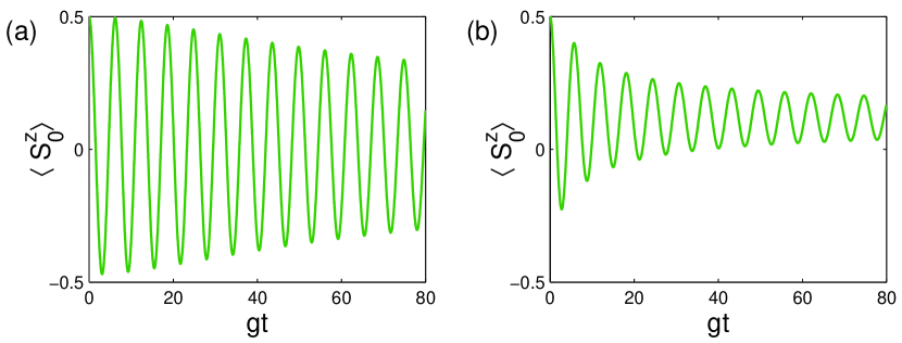
Figure 1: Time evolution of $\langle S_{0}^{z}\rangle$ for different values of (a) $\Omega=2$ and (b) $\Omega=30$. The initial qubit state is $|\psi(0)\rangle=|1\rangle$ and other parameters are $\varepsilon=0$ and $J_{0}=0.05g$.

In this section, we present and discuss the results we obtain. We first study the dynamics of the central spin inversion. Figures 1(a) and 1(b) show the time evolution of $\langle S_{0}^{z}\rangle$ for different values of $\Omega$ in the case of resonance (i.e., detuning $\varepsilon=0$). Figure 2(a) shows the time evolution of $\langle S_{0}^{z}\rangle$ also in resonance (i.e., detuning $\varepsilon=0$) but with a different value of the system-environment coupling strength $J_{0}$ from that of Fig. 1(a). For the parameters chosen in Figs. 1(a), 1(b) and 2(a), the driving strength $g$ is much larger than the coupling strength, i.e., $g\gg J_{0}$. As a result, the self-Hamiltonian is dominant over the interaction with the environment. The eigenstates of the self-Hamiltonian are $|+\rangle=(|1\rangle+|0\rangle)/\sqrt{2}$ and $|-\rangle=(|1\rangle-|0\rangle)/\sqrt{2}$, separated by a large Rabi frequency $g$. The main influence of the environment on the central spin is to destroy the initial phase relation between the states $|+\rangle$ and $|-\rangle$. This leads to the decay of $\langle S_{0}^{z}\rangle$, i.e., Rabi oscillation decay. From Figs. 1(a) and 2(a), we can see that as expected, increasing the value of $J_{0}$ results in the increase of the decay rate of the Rabi oscillations. Apart from the coupling constant $J_{0}$, the important factor $\Omega$, Eq. (26), also reflects the influence of the environment on the central spin as shown in Fig. 1(b). We can see from Figs. 1(a), 1(b) and 2(a) that increasing the factor $\Omega$ and increasing the coupling constant $J_{0}$ have similar effects. One can observe that the larger the value of $\Omega$ is, the stronger the decay of the amplitude of the Rabi oscillations will be. As in the case of the spin-boson model discussed in Ref. [56], the central spin inversion does not oscillate around the value of $\langle S_{0}^{z}\rangle=0$. Its oscillations are, however, biased (shifted) a little bit toward the positive value of the initial $\langle S_{0}^{z}(0)\rangle$. With the increase of the value of $\Omega$ or $J_{0}$, this effect is enhanced.

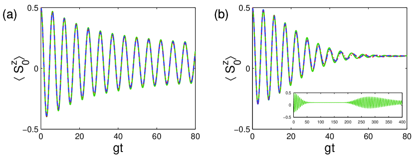
Figure 2: (a) Time evolution of $\langle S_{0}^{z}\rangle$ for different values of $\Omega=2$, $J_{0}=0.1g$ (green solid curve), $\Omega=2\times 10$, $J_{0}=0.1g/\sqrt{10}$ (blue dashed curve) and $\Omega=2\times 100$, $J_{0}=0.1g/\sqrt{100}$ (red dotted curve). The initial qubit state is $|\psi(0)\rangle=|1\rangle$ and the other parameter is $\varepsilon=0$. (b) Time evolution of $\langle S_{0}^{z}\rangle$ for different values of $\Omega=1$, $J_{0}=0.05g$ (green solid curve), $\Omega=1\times 10$, $J_{0}=0.05g/\sqrt{10}$ (blue dashed curve) and $\Omega=1\times 100$, $J_{0}=0.05g/\sqrt{100}$ (red dotted curve). The initial qubit state is $|\psi(0)\rangle=|1\rangle$ and the other parameter is $\varepsilon=0.5g$. The inset shows the time evolution of the case of $\Omega=1$ and $J_{0}=0.05g$ in a larger time interval.

It was shown in Ref. [17] that the form and the rate of Rabi oscillation decay are useful in experimentally determining the intrabath coupling strength for a broad class of solid-state systems [17]. This is also the case in our problem. The central spin is a two-level system. However, due to its interaction with the environment, the time evolution of the central spin inversion consists of different frequencies involved in the time series of Eqs. (40)–(42) as well as Eqs. (33)–(35). The frequencies from Eq. (35) can be written as

$$\kappa=\sqrt{\left[J_{0}(P_{2}-P_{1})-\varepsilon\right]^{2}+g^{2}}$$ (62)

for a pair of integers $P_{1}$ and $P_{2}$. The probability distribution of the frequencies is then

$$\sigma(\kappa)=\frac{1}{Z}\sum_{P=0}^{\infty}\Lambda(P+n)\Lambda(P),$$ (63)

where $n=|P_{2}-P_{1}|$. It is possible that other pairs of integers $P^{\prime}_{1}$ and $P^{\prime}_{2}$ may exist which correspond to the same frequency $\kappa$ but with $m=|P^{\prime}_{2}-P^{\prime}_{1}|\neq n$. In such case, we should add an additional probability

$$\sigma(\kappa)=\frac{1}{Z}\sum_{P=0}^{\infty}\Lambda(P+m)\Lambda(P).$$ (64)

For example, the frequencies of Eq. (62) can be rewritten as

$$\kappa=\sqrt{J_{0}\left[(P_{2}-P_{1})-(\varepsilon/J_{0})\right]^{2}+g^{2}}.$$ (65)

If $n=|P_{2}-P_{1}|$ is chosen to be $3$, then other pairs of integers $P^{\prime}_{1}$ and $P^{\prime}_{2}$ with $m=|P^{\prime}_{2}-P^{\prime}_{1}|=17$ correspond to the same frequency $\kappa$ for the parameters $\varepsilon=0.5g$ and $J_{0}=0.05g$ used in Fig. 2(b). Thus, summing the probability distributions with all possible combinations of $P_{1}$ and $P_{2}$ that correspond to the same frequency $\kappa$ leads to the final frequency probability distribution.

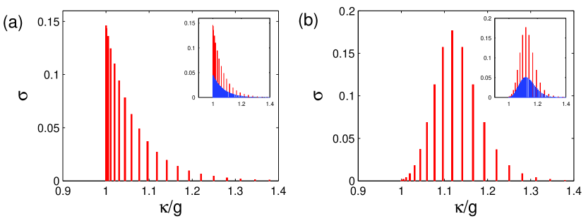
Figure 3: (a) Probability distribution of frequencies for $\varepsilon=0$, $\Omega=5$, and $J_{0}=0.05g$. The inset shows the comparison between the probability distribution of frequency and that of the case of increasing $N$ $10$ times (i.e., $\Omega=5\times 10$, $J_{0}=0.05g/\sqrt{10}$) with other parameters unchanged. (b) Probability distribution of frequencies for the parameters used in Fig. 2(b). The inset shows the comparison between the probability distribution of frequencies and that of the case of increasing $N$ 10 times (i.e., $\Omega=1\times 10$, $J_{0}=0.05g/\sqrt{10}$) with other parameters unchanged.

Figure 3(a) shows the frequency probability distribution for the case of $\varepsilon=0$, $J_{0}=0.05g$, and $\Omega=5$. It is obvious that the main frequencies are located near $g$ which is approximately the Rabi frequency. This is also the case for Figs. 1(a), 1(b) and 2(a) where the detuning $\varepsilon=0$. The contribution of many different frequencies, a consequence of interacting with the AF bath, results in the Rabi oscillation decay of the central spin. For the case of non-zero detuning $\varepsilon=0.5g$, Fig. 2(b), with $J_{0}=0.05g$ and $\Omega=1$, shows a decay of oscillations with an approximated Rabi frequency of $\sqrt{\varepsilon^{2}+g^{2}}\approx 1.12g$. The oscillation residual amplitude approaches almost zero for a time period of about $65\leq gt\leq 80$ [see also the inset of Fig. 2(b)]. In such case, different frequencies interfere with each other and produce the zero amplitude variation period, a behavior that is called collapse in quantum optics [58]. At longer times, the oscillation amplitude revives. This is shown clearly in the inset of Fig. 2(b). Reference [47] reported an experimental observation of a similar collapse and revival phenomenon for driven spin oscillations, though the spin bath and the corresponding interactions are different from those discussed here.

The environmental conditions affect the dynamics of the central spin and the completeness of the collapse. Figure 3(b) shows the frequency probability distribution for the central spin inversion with parameters used in Fig. 2(b). The distribution has a left-hand-side cutoff at $\kappa_{min}=g$ and the center of the distribution is located at $\kappa_{c}=\sqrt{\varepsilon^{2}+g^{2}}$. One can easily understand this from the frequency relation Eq. (62). It is also obvious from Eq. (62) that the center of the distribution shifts toward larger frequencies with the increase of the detuning [this can also be seen from the comparison between Figs. 3(a) and 3(b)]. If the detuning $\varepsilon$ exists, it is possible that the shape of the frequency probability distribution becomes approximately Gaussian, which then results in well-defined collapse and revival behavior regions [56]. If the detuning is zero, only a half side of the distribution exists [see Fig. 3(a)] and the central spin inversion will never show the (complete) collapse and revival behaviors. The frequency probability distribution is determined also by the coupling strength $J_{0}$ and the important factor $\Omega$. With the increase of $J_{0}$ or $\Omega$, the width of frequency distribution increases and the probability decreases. As a result, the decay of the Rabi oscillations is enhanced.

We note that the results presented here depend, of course, on the number of environment atoms $N$ in each sublattice. The influence of the number of atoms $N$ in each sublattice on the dynamics of the central spin comes from two respects. One is the scaled coupling constant $J_{0}=J^{\prime}_{0}//\sqrt{N}$ which is proportional to $1/\sqrt{N}$. The other is the factor $\Omega$, Eq. (26), which is proportional to $N$. We plot in Fig. 2(a) and Fig. 2(b) the time evolutions of $\langle S_{0}^{z}\rangle$ in (blue) dashed curve and (red) dotted curve corresponding, respectively, to increasing $N$ by 10 and 100 times but keeping other parameters unchanged. The results show that the two curves in dashed and dotted lines almost coincide with each other. If we increase $N$ by 200 times, then the resultant evolution and that of increasing $N$ by 100 times become indistinguishable and converge toward the same evolution. In other words, a nontrivial finite limit exists in the thermodynamic limit of $N\rightarrow\infty$. This has been shown analytically in Refs. [26, 27, 28] for a spin coupled to an AF environment without an external ac driving field. We show numerically here that this $N\rightarrow\infty$ limit also exists in the driven spin case. One can also notice that the difference between the original curve (in solid line) and the two curves (in dashed and dotted lines, respectively) in Fig. 2 is very small in the all time interval shown. This difference in Fig. 2(b) with $\varepsilon\neq 0$ is also small but is slightly larger at large times. These indicate that the results presented here are very close to the results in the thermodynamic limit. If we also increase the AF atom number $N$ in $J_{0}$ and $\Omega$ simultaneously but keep other parameters unchanged, then we can find that the number of the contributed frequencies in the probability distribution of frequencies becomes larger (i.e., the separation between two adjacent distributed frequencies becomes smaller or denser) and the value of the distribution becomes smaller [see the insets in Figs. 3(a) and 3(b)]. But the width and the shape of the frequency probability distribution remain almost the same as before [see the insets in Figs. 3(a) and 3(b)]. The fact that the frequency distribution does not change much results in the very similar dynamics of the driven spin (see Fig. 2) when we increase $N$. The existence of nontrivial finite limits as $N\rightarrow\infty$ and the small difference between the original dynamical evolutions with their counterparts in the thermodynamic limit are true for all the dynamic variables ($\langle S_{0}^{z}\rangle$ and von Neumann entropy) presented in this article.

3.2 von Neumann entropy

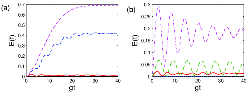
Figure 4: (a) Entropy $E(t)$ for different initial qubit states: $|\psi(0)\rangle=(|\varphi_{1}\rangle+|\varphi_{2}\rangle)/\sqrt{2}$ (pink dot-dashed curve), $|\psi(0)\rangle=|1\rangle$ (blue dashed curve), $|\psi(0)\rangle=|\varphi_{1}\rangle$ or $|\psi(0)\rangle=|\varphi_{2}\rangle$ (red solid curve). Other parameters are $\varepsilon=g$, $J_{0}=0.01g$, $\Omega=20$. (b) Entropy $E(t)$ for (i) pink dot-dashed curve: $J_{0}=0.03g$, $\varepsilon=0$, (ii) green dashed curve: $J_{0}=0.01g$, $\varepsilon=0$, (iii) red solid curve: $J_{0}=0.01g$, $\varepsilon=g$, and (iv) blue dotted curve: $J_{0}=0.01g$, $\varepsilon=3g$. The qubit initial state is $|\psi(0)\rangle=|\varphi_{1}\rangle$ or $|\psi(0)\rangle=|\varphi_{2}\rangle$, and other parameter is $\Omega=20$.

The purity of a mixed state can be measured by the von Neumann entropy

$$E(t)=-\textrm{tr}_{S}[\rho_{S}(t)\ln\rho_{S}(t)].$$ (66)

After diagonalizing the reduced density matrix $\rho_{S}(t)$, we obtain the von Neumann entropy

$$E(t)=-\sum_{k=1}^{2}p_{k}(t)\ln p_{k}(t),$$ (67)

where $p_{k}(t)$ are the eigenvalues of the reduced density matrix $\rho_{S}(t)$ and can be expressed as

$$p_{1,2}(t)=\frac{\rho_{11}(t)+\rho_{22}(t)\pm\sqrt{[\rho_{11}(t)-\rho_{22}(t)]^{2}+4\rho_{12}(t)\rho_{21}(t)}}{2}.$$ (68)

We investigate the von Neumann entropy of the qubit system in Fig. 4. In Fig. 4(a), for the initial state $|\psi(0)\rangle=|1\rangle$, the entropy $E(t)$ oscillatorily approaches its maximal value of 0.4228 (in blue dashed curve). If the initial state is one of the eigenstates of the qubit self-Hamiltonian, i.e., $|\varphi_{1}\rangle$ or $|\varphi_{2}\rangle$, the von Neumann entropy $E(t)$ remains small with time and approaches a very small value in the long-time limit (in red solid line). In the opposite, if we choose the superposition state $|\psi(0)\rangle=(|\varphi_{1}\rangle+|\varphi_{2}\rangle)/\sqrt{2}$ as the initial state, results show that the von Neumann entropy $E(t)$ increases monotonously to the maximal value of $\ln 2=0.6971$ (in pink dot-dashed line), representing a completely mixed state. That is to say, this initial state gets maximally entangled with the environment in the course of the evolution. This initial superposition state is thus frangible to the influence of the environment and should be avoided being used in the quantum information processing in the presence of the AF environment. In all the cases, the entropy $E(t)$ increases with the increase of the factor $\Omega$ and the coupling constant strength $J_{0}$.

We discuss next the pointer states of the qubit from the perspective of the von Neumann entropy [59, 60, 61]. For $g=0$, i.e., no driving field, it is obvious that the eigenstates of the self-Hamiltonian, $\mu_{0}S_{0}^{z}$, are the pointer states as the self-Hamiltonian commutes with the interaction Hamiltonian with the environment. In this case, a generic quantum state decays, after the decoherence time, into a mixture of pointer states. Thus the decoherence behavior can be described effectively by the off-diagonal elements (decoherence factor) of the reduced density matrix in the pointer state basis of the system. This is exactly the cases studied in Refs. [26, 27], where the off-diagonal elements (decoherence factor) vanish in the long-time limit in the eigenstate basis of the self-Hamiltonian or of the interaction Hamiltonian with the environment regardless of the different initial states. If the driving field strength $g\neq 0$, it is difficult to identify the exact pointer states of the system (especially in the non-perturbative and non-Markovian regime) as the self-Hamiltonian does not commute with the interaction Hamiltonian with the bath. Pointer states may be defined as the states which become minimally entangled with the environment in the course of their evolution [59, 60]. An operational definition in terms of the von Neumann entropy, introduced in Refs. [59, 60, 61], is that pointer states are obtained by minimizing the von Neumann entropy over the initial state $|\psi(0)\rangle$ and requiring that the answer be robust when varying the time $t$. In general situations, pointer states result from the interplay between self-evolution and interaction with the environment, and thus their dynamical selection by the environment are complicated. For $g>>J_{0}$ or/and $\varepsilon>>J_{0}$, the pointer states turn out (approximately) to be the eigenstates of the self-Hamiltonian [24, 59]. Here the eigenstates $|\varphi_{1}\rangle$ and $|\varphi_{2}\rangle$ of the self-Hamiltonian $H_{S}=\varepsilon S_{0}^{z}+gS_{0}^{x}$ defined in Eq. (5) can be written as

$$\left(\begin{array}[]{c}|\varphi_{1}\rangle\\ |\varphi_{2}\rangle\end{array}\right) = U\left(\begin{array}[]{c}|1\rangle\\ |0\rangle\end{array}\right)$$ (73)

$$= \left(\begin{array}[]{cc}U_{11}&U_{12}\\ U_{21}&U_{22}\end{array}\right)\left(\begin{array}[]{c}|1\rangle\\ |0\rangle\end{array}\right),$$ (78)

where

$$U_{11} = \frac{1}{\sqrt{2}}\frac{g}{\sqrt{\varepsilon^{2}+g^{2}-\varepsilon\sqrt{\varepsilon^{2}+g^{2}}}},$$ (79)

$$U_{12} = \frac{1}{\sqrt{2}}\frac{\sqrt{\varepsilon^{2}+g^{2}}-\varepsilon}{\sqrt{\varepsilon^{2}+g^{2}-\varepsilon\sqrt{\varepsilon^{2}+g^{2}}}},$$ (80)

$$U_{21} = \frac{1}{\sqrt{2}}\frac{g}{\sqrt{\varepsilon^{2}+g^{2}+\varepsilon\sqrt{\varepsilon^{2}+g^{2}}}},$$ (81)

$$U_{22} = -\frac{1}{\sqrt{2}}\frac{\sqrt{\varepsilon^{2}+g^{2}}+\varepsilon}{\sqrt{\varepsilon^{2}+g^{2}+\varepsilon\sqrt{\varepsilon^{2}+g^{2}}}}.$$ (82)

Thus for the Hamiltonian parameters chosen in Fig. 4(a) which is in a regime where the self-Hamiltonian of the system dominates, it is expected that the pointer states are very close to the eigenstates $|\varphi_{1}\rangle$ and $|\varphi_{2}\rangle$ [24, 59]. By changing different initial states near the eigenstates $|\varphi_{1}\rangle$ or $|\varphi_{2}\rangle$ with other parameters fixed, it is found that the eigenstate $|\varphi_{1}\rangle$ or $|\varphi_{2}\rangle$ produces the minimum entropy increase with time (the red solid line). This suggests that the eigenstates $|\varphi_{1}\rangle$ and $|\varphi_{2}\rangle$ are dynamically selected by the environment as the preferred pointer states in the self-Hamiltonian dominant regime. Moreover, when the energy parameters $g$ and $\varepsilon$ of the self-Hamiltonian of the central spin system are increased further with respect to the system-bath coupling strength $J_{0}$ (i.e., the self-Hamiltonian dominates even more), the values of entropy evolution are lower (the green dashed curve is lower than the pink dot-dashed curve in the zero-detuning case, and the blue dotted curve that is close to zero is lower than the red solid curve in the detuning case) as shown in Fig. 4(b). We have also checked that the four curves with initial state $|\varphi_{1}\rangle$ or $|\varphi_{2}\rangle$ in Fig. 4(b) are, respectively, the minimum entropy curves in the course of evolution among those entropy evolution curves with initial states varied near the eigenstate of $|\varphi_{1}\rangle$ or $|\varphi_{2}\rangle$ but with other parameters fixed. This confirms furthermore again that in the regime where the self-Hamiltonian of the system dominates (with or without detuning), the eigenstates of the system self-Hamiltonian emerge as the preferred pointer states.

4 Conclusions

We investigate the decoherence of a qubit in an AF environment, in the presence of a driving field. The difficulty of our problem lies in the fact that the self-Hamiltonian does not commute with the interaction Hamiltonian and the internal dynamics (coupling) of the spin bath are taken into consideration at the same time. The spin-wave approximation is used to map the spin operators of the AF environment onto bosonic operators in the low-temperature and low-excitation limit. Then the resultant model is solved exactly, even in the case of multi-environment modes and finite environment temperatures. Our approach includes the environment dynamics, the qubit dynamics, and the quantum correlations between them. The influence of the AF environment on the qubit is found to depend on two factors, i.e., the coupling constant $J_{0}$ and a dimensionless factor $\Omega=\frac{NT^{3}}{4\sqrt{2}\pi^{2}M^{3/2}J^{3}}$. Increasing the two factors, the decay time of the Rabi oscillations becomes shorter, the decoherence of the qubit is enhanced, and the qubit state becomes more mixed with time. The time evolution of the Rabi oscillations also depends on the detuning between the driving frequency and the qubit Larmor frequency. If the detuning exists, the Rabi oscillations may show a behavior of collapses and revivals; however, if the detuning is zero, such a behavior will not appears. This can be understood in terms of the weighted frequency distribution investigated here. Also the decoherence and the pointer states of the qubit are discussed from the perspective of the von Neumann entropy. It is found that the eigenstates of the qubit self-Hamiltonian are dynamically selected by the environment as the preferred pointer states in the weak system-environment coupling limit (or in the self-Hamiltonian dominant regime).

References

References

- [1] B. E. Kane, Nature (London) 393, 133 (1998).
- [2] H.-S. Goan, Int. J. Quantum Inf. 3, 27 (2005); L. C. L. Hollenberg et al., Phys. Rev. B 74, 045311 (2006); C. J. Wellard et al., ibid. 68, 195209 (2003); B. Koiller et al., Phys. Rev. Lett. 88, 027903 (2001); L. M. Kettle et al., Phys. Rev. B 73, 115205 (2006).
- [3] C. D. Hill and H.-S. Goan, Phys. Rev. A 68, 012321 (2003). C. D. Hill and H.-S. Goan, Phys. Rev. A 70, 022310 (2004); L. M. Kettle et al., Phys. Rev. B 68, 075317 (2003).
- [4] D.-B. Tsai, P.-W. Chen, and H.-S. Goan, Phys. Rev. A 79, 060306(R) (2009). C. D. Hill et al., Phys. Rev. B 72, 045350 (2005).
- [5] G. Burkard, D. Loss, and D. P. DiVincenzo, Phys. Rev. B 59, 2070 (1999).
- [6] R. Raussendorf and H. J. Briegel, Phys. Rev. Lett. 86, 5188 (2001).
- [7] X. Hu and S. Das Sarma, Phys. Rev. Lett. 96, 100501 (2006).
- [8] D. Loss and D. P. DiVincenzo, Phys. Rev. A 57, 120 (1998).
- [9] V. Cerletti, W. A. Coish, O. Gywat, and D. Loss, Nanotechnology 16 R27 (2005).
- [10] M. Borhani, V. N. Golovach, and D. Loss, Phys. Rev. B 73, 155311 (2006).
- [11] A. Tackeuchi, T. Kuroda, K. Yamaguchi, Y. Nakata, N. Yokoyama, and T. Takagahara, Physica E 32, 423 (2006).
- [12] L. Cywinski, W. M. Witzel, and S. Das Sarma, Phys. Rev. B 79, 245314 (2009).
- [13] W. Zhang, N. P. Konstantinidis, V. V. Dobrovitski, B. N. Harmon, L. F. Santos, and L. Viola, Phys. Rev. B 77, 125336 (2008).
- [14] W. Zhang, V. V. Dobrovitski, K. A. Al-Hassanieh, E. Dagotto, and B. N. Harmon, Phys. Rev. B 74, 205313 (2006).
- [15] W. Zhang, V. V. Dobrovitski, L. F. Santos, L. Viola, and B. N. Harmon, Phys. Rev. B 75, 201302 (2007).
- [16] J. Lages, V. V. Dobrovitski, M. I. Katsnelson, H. A. De Raedt, and B. N. Harmon, Phys. Rev. E 72, 026225 (2005).
- [17] V. V. Dobrovitski, A. E. Feiguin, R. Hanson, and D. D. Awschalom, Phys. Rev. Lett. 102, 237601 (2009).
- [18] S. Takahashi, R. Hanson, J. van Tol, M. S. Sherwin, and D. D. Awschalom, Phys. Rev. Lett. 101, 047601 (2008).
- [19] W. Yang and R.-B. Liu, Phys. Rev. B 78, 085315 (2008).
- [20] W. Yang and R.-B. Liu, Phys. Rev. B 79, 115320 (2009).
- [21] W. M. Witzel and S. Das Sarma, Phys. Rev. B 74, 035322 (2006).
- [22] V. V. Dobrovitski and H. A. De Raedt, Phys. Rev. E 67, 056702 (2003).
- [23] K. A. Al-Hassanieh, V. V. Dobrovitski, E. Dagotto, and B. N. Harmon, Phys. Rev. Lett. 97, 037204 (2006).
- [24] F. M. Cucchietti, J. P. Paz, and W. H. Zurek, Phys. Rev. A 72, 052113 (2005).
- [25] J. Dziarmaga, Phys. Rev. B 71, 054516 (2005).
- [26] X. Z. Yuan and K. D. Zhu, Europhys. Lett. 69, 868 (2005).
- [27] X. Z. Yuan, H. S. Goan, and K. D. Zhu, New J. Phys. 9, 219 (2007).
- [28] X. Z. Yuan, H.-S. Goan, and K. D. Zhu, Phys. Rev. A 81, 034102 (2010).
- [29] E. Novais, A. H. Castro Neto, L. Borda, I. Affleck, G. Zarand, Phys. Rev. B 72, 014417 (2005).
- [30] H. P. Breuer, Phys. Rev. A 69, 022115 (2004).
- [31] A. Hutton and S. Bose, Phys. Rev. A 69, 042312 (2004).
- [32] M. Lucamarini, S. Paganelli, S. Mancini, Phys. Rev. A 69, 062308 (2004).
- [33] H. P. Breuer, D. Burgarth, and F. Petruccione, Phys. Rev. B 70, 045323 (2004).
- [34] Y. Hamdouni, M. Fannes, and F. Petruccione, Phys. Rev. B 73, 245323 (2006).
- [35] X. Z. Yuan, H.-S. Goan, K. D. Zhu, Phys. Rev. B 75, (2007).
- [36] H. T. Quan, Z. Song, X. F. Liu, P. Zanardi, C. P. Sun, Phys. Rev. Lett. 96, 140604 (2006).
- [37] F. M. Cucchietti, S. F. Vidal, J. P. Paz, Phys. Rev. A 75, 032337 (2007).
- [38] D. Rossini, T. Calarco, V. Giovannetti, S. Montangero, R. Fazio,, Phys. Rev. A 75, 032333 (2007).
- [39] H. Krovi, O. Oreshkov, M. Ryazanov, and D. A. Lidar, Phys. Rev. A 76, 052117 (2007).
- [40] E. Ferraro, H.-P. Breuer, A. Napoli1, M. A. Jivulescu, and A. Messina Phys. Rev. B 78, 064309 (2008)
- [41] N. Arshed, A. H. Toor, and D. A. Lidar, Phys. Rev. A 81, 062353 (2010)
- [42] J. R. Petta, A. C. Johnson, J. M. Taylor, E. A. Laird, A. Yacoby, M. D. Lukin, C. M. Marcus, M. P. Hanson, and A. C. Gossard , Science 309, 2180 (2005).
- [43] M. H. Mikkelsen, J. Berezovsky, N. G. Stoltz, L. A. Coldren, and D. D. Awschalom, Nature Phys. 3, 770 (2007).
- [44] F. H. L. Koppens, C. Buizert, K. J. Tielrooij, I. T. Vink, K. C. Nowack, T. Meunier, L. P. Kouwenhoven, and L. M. K. Vandersypen, Nature (London) 442, 766 (2006).
- [45] B. C. Stipe, H. J. Mamin, C. S. Yannoni, T. D. Stowe, T. W. Kenny, and D. Rugar, Phys. Rev. Lett. 87, 277602 (2001).
- [46] F. H. L. Koppens, D. Klauser, W. A. Coish, K. C. Nowack, L. P. Kouwenhoven, D. Loss, and L. M. K. Vandersypen, Phys. Rev. Lett. 99, 106803 (2007).
- [47] R. Hanson, V. V. Dobrovitski, A. E. Feiguin, O. Gywat, D. D. Awschalom, Science 320, 352 (2008).
- [48] D. D. Bhaktavatsala Rao, Phys. Rev. A 76, 042312 (2007).
- [49] M. Lucamarini, S. Paganelli, and S. Mancini, Phys. Rev. A 69, 062308 (2004).
- [50] A. Lupaşcu, E. F. C. Driessen, L. Roschier, C. J. P. M. Harmans, and J. E. Mooij, Phys. Rev. Lett. 96, 127003 (2006).
- [51] C. Kittel, Quantum Theory of Solids, (John Wiley and Sons, Inc., New York, 1963).
- [52] H. P. Breuer, D. Burgarth, and F. Petruccione, Phys. Rev. B 70, 045323 (2004).
- [53] M. Frasca, Ann. Phys. N.Y. 313, 26 (2004).
- [54] K. Yosida, Theory of Magnetism, (Springer series in solid-state sciences, V. 122).
- [55] A. J. Leggett, S. Chakravarty, A. T. Dorsey, M. P. A. Fisher, A. Garg and W. Zwerger, Rev. Mod. Phys. 59, 1 (1987)
- [56] E. K. Irish, J. Gea-Banacloche, I. Martin, and K. C. Schwab, Phys. Rev. B 72, 195410 (2005).
- [57] H. Xiong, S. Liu, G. Huang, and Z. Xu, Phys. Rev. A 65, 033609 (2002).
- [58] M. O. Scully, M. S. Zubairy, Quantum Optics, (Cambridge University Press, Cambridge, 1997).
- [59] J. P. Paz, and W. H. Zurek, Phys. Rev. Lett. 82, 5181 (1999).
- [60] W. H. Zurek, S. Habib, and J. P. Paz, Phys. Rev. Lett. 70, 1187 (1993).
- [61] W. H. Zurek, Rev. Mod. Phys. 75, 715 (2003).