Unified Spin Order Theory via Gauge Landau-Lifshitz Equation

Abstract

The continuum limit of the tilted SU(2) spin model is shown to give rise to the gauge Landau-Lifshitz equation which provides a unified description for various spin orders. For a definite gauge, we find a double periodic solution, where the conical spiral, in-plane spiral, helical, and ferromagnetic spin orders become special cases, respectively. For another gauge, we obtain the skyrmion-crystal solution. By simulating the influence of magnetic field and temperature for our covariant model, we find a spontaneous formation of skyrmion-fragment lattice and obtain a wider range of skyrmion-crystal phase in comparison to the conventional Dzyaloshinsky-Moriya model.

There has been spectacular progress in the study on the magnetoelectric effects, which is expected to make a realistic step toward an electrical control of magnetismFiebig ; Tokura06 ; Eerenstein ; Choi . Within the intertwining of theory and experiment, a mechanism based on spin-current showed that the enhanced ferroelectric domains can be realized through cycloidal and conical spin states in certain materials Tokura06 ; Nag . For example, spiral spin state was shown Nag to cause electronic polarization. Moreover, complex spin texture is interesting by its own right. Recently, skyrmion lattice is observed in bulk MnSi Muh and thin film $\mathrm{Fe}_{x}\mathrm{Co}_{1-x}\mathrm{Si}$ Tokura . Magnons in helical magnets are also probed by neutron scattering experiments heliband . Those nontrivial spin textures, undoubtedly, play an important role in novel multiferroic materials. There are mainly two kinds of mechanisms that cause spiral spin state, one is ferro/antiferro-magnetic exchange competition that is believed to be the origin of spiral state in manganites j1j2j3 , the other is the antisymmetric Dzyaloshinsky-Moriya (DM) interaction Dzyaloshinskii ; Moriya which arises from spin-orbit (SO) interaction and manifests in crystal without inversion symmetry like MnSi. Historically, Moriya Moriya was the first to give a microscopic treatment of DM interaction based on Anderson’s superexchange mechanism with SO interaction. Thirty two years later, Shekhtman isodm found that Moriya’s theory has a bond-isotropic form if only one takes all the terms up to second order in SO interaction which is usually neglected until present. It is important to set up a unified description for various spin orders.

In this letter, we indicate that such a system can be described by tilted Heisenberg model in which the tilting is related to the effects associated with bonds. We formulate gauge Landau-Lifshitz equation from this model and find solutions of various spin textures and derive the dispersion relation of the relevant spin waves, which provides a unified theory for spin orders with insight in the gauge and geometric point of view. Then we investigate the influence of external magnetic field and temperature and plot the corresponding phase diagram by making use of Monte Carlo simulations.

In order to reach a unified description of various spin ordered phases including the situations beyond the traditional ferromagnetic one, we consider a much more generalized Heisenberg Hamiltonian

$$H=-J\sum_{\langle jj^{\prime}\rangle,c}U_{j}S^{c}_{j}U^{-1}_{j}\,U_{j^{\prime}}S^{c}_{j^{\prime}}U^{-1}_{j^{\prime}}$$ (1)

where $c=1,2,3$, $j\in L$ with $L$ the lattice space, and $S^{c}_{j}$ denotes the $c$-th component of spin operator at site $j$. These spin operators, proportional to the infinitesimal generators of SU(2), obey $[S^{a}_{j},~{}S^{b}_{l}]=i\hbar\delta_{jl}\epsilon^{abc}S^{c}_{j}$ that governs the time developments of any observable via Heisenberg equation of motion for a definite model (1). In Eq. (1), $\langle jj^{\prime}\rangle$ means the summation is taken over the nearest neighbor lattice sites, and the local tilting field $U_{j}$ accounts for any effects arising from either (both) complicated crystalline fields or (and) cumbersome charge order in whatever intricate materials.

As there exists a homomorphism between SU(2) and SO(3) Lie groups, $U_{j}\bm{S}_{j}U^{-1}_{j}=\bm{S}_{j}O_{j}$ in which $\bm{S}_{j}$ denotes $(S^{1}_{j},S^{2}_{j},S^{3}_{j})$ and $O_{j}$ the representation of SO(3), each nearest-neighbor term in Eq. (1) can be rearranged, i.e., $\displaystyle\sum_{c}U_{j}S^{c}_{j}U^{-1}_{j}\,U_{j^{\prime}}S^{c}_{j^{\prime}}U^{-1}_{j^{\prime}}=\bm{S}_{j}O_{j}(\bm{S}_{j^{\prime}}O_{j^{\prime}})^{\small T}=\bm{S}_{j}O_{j}O_{j^{\prime}}^{-1}\bm{S}_{j^{\prime}}^{\small T}$. Here $O_{j^{\prime}}^{\small T}=O_{j^{\prime}}^{-1}$ for orthogonal group has been used. Because $j^{\prime}$ is close to $j$ when the lattice constant $a$ is taken as an infinitesimal parameter, we can expend $O_{j}O_{j^{\prime}}^{-1}$ in the vicinity of identity, namely

$$O_{j}O_{j^{\prime}}^{-1}=1-aA^{c}_{\nu}(j)\,\hat{\ell}_{c},$$ (2)

where we have considered the coordinate of site $j^{\prime}$ is simply that of $j$ plus a bond vector $a\bm{e}_{\nu}$ in which $\bm{e}_{\nu}$ refers to the unit vectors connecting neighborhood of a given lattice structure. Here $\hat{\ell}_{c}$ denote the representation matrices of the infinitesimal generators of SO(3) Lie group, they are $3\times 3$ matrices $(\hat{\ell}_{c})_{ab}=\epsilon_{abc}$ and fulfil the commutation relations Gilmore $[\hat{\ell}_{a}\,,\hat{\ell}_{b}]=-\epsilon_{abc}\hat{\ell}_{c}$. Clearly, the feature of the local tilting can be characterized by the SO(3) non-Abelian gauge potential $\mathbb{A}_{\nu}(j)=A^{c}_{\nu}(j)\hat{\ell}_{c}$ which is a matrix valued vector field. In order to avoid any ambiguity, here we clarify that the $j$ represents a point in the lattice space corresponding to the coordinate of real space in continuum model, the $c$ labels the component of a vector in Lie algebra space while the $\nu$ labels the one in real space. Also for symbol neatness, in Eq. (2) and thereafter, we write the lattice-site label $j$ of $\bm{A}$ in parentheses rather than conventional subscripts. By making use of Eq. (2), we can write Eq. (1) as

$$H=\frac{J}{2}\sum_{\langle jj^{\prime}\rangle}\left[\Bigl{(}\bm{S}_{j^{\prime}}-\bm{S}_{j}+a\bm{S}_{j}A^{c}_{\nu}(j)\,\hat{\ell}_{c}\Bigr{)}^{2}-2C_{j}\right].$$ (3)

Actually, the Casimir invariants $C_{j}=\bm{S}_{j}\cdot\bm{S}_{j}=s_{j}(s_{j}+1)\hbar^{2}$ in a general system may differ at different lattice site, which means the module of spin does not necessarily take the same value everywhere. However, in this paper, we focus on uniform spin module $S$ in every sites.

Now we are in the position to make continuum limit, $\sum\rightarrow(1/a)^{d}\int d^{d}x$, which can be realized by allowing the volume per lattice site $a^{d}$ tend to zero and considering the lattice label $j$ as a continuous variable $\bm{r}$ and hence $\bm{S}_{j}$ as $\bm{M}(\bm{r})$. Equation (3) gives rise to the effect Hamiltonian,

$$H=\frac{J}{2a^{d-2}}\int d^{d}x\Big{[}\bigl{(}\partial_{\nu}+\bm{A}_{\nu}(\bm{r})\times\bigr{)}\bm{M}(\bm{r})\Bigr{]}^{2},$$ (4)

where the additional constant term is omitted. Then the corresponding Lagrangian density is given by ${\mathscr{L}}=a^{-d}|\bm{M}|(\cos\theta-1)\dot{\phi}-a^{2-d}J/2\,(D\bm{M})^{2}$ in which $(\theta,\phi)$ refer to the azimuthal angles of $\bm{M}$. The equation of motion for the spin field $\bm{M}(\bm{r},t)$ is derived as the following gauge Landau-Lifshitz equation,

$$\frac{\partial}{\partial t}\bm{M}=a^{2}J\bm{M}\times D^{2}\bm{M},$$ (5)

where $D^{2}=D_{\nu}D_{\nu}$ and the covariant derivative is given by $D_{\nu}\bm{M}=(\partial_{\nu}+\bm{A}_{\nu}\times)\bm{M}$. Equation (5) is covariant under a gauge transformation $\mathbb{A}_{\nu}\rightarrow G\mathbb{A}_{\nu}G^{-1}+\partial_{\nu}GG^{-1}$, $(\bm{M})_{a}\rightarrow\sum_{b}G_{ab}(\bm{M})_{b}$ with $G\in\mathrm{SO(3)}$.

We first consider a typical gauge field in $x$-$y$ plane $\bm{A}_{x}=(0,0,-q_{1})$, $\bm{A}_{y}=(q_{2}\sin q_{1}x,-q_{2}\cos q_{1}x,0)$. We find a double periodic solution, $\bm{M}_{\mathrm{dp}}$, as a steady solution of the gauge Landau-Lifshitz equation (5),

$$\left\{\begin{array}[]{l}m_{1}(x,y)=\sin(q_{2}y+\beta)\cos(q_{1}x),\\[2.84526pt] m_{2}(x,y)=\sin(q_{2}y+\beta)\sin(q_{1}x),\\[2.84526pt] m_{3}(x,y)=\cos(q_{2}y+\beta).\end{array}\right.$$ (9)

Here $\bm{m}=(m_{1},m_{2},m_{3})$ refers to $\bm{M}_{\mathrm{dp}}/S$. This spin order is the exact ground-state solution of the system because $D_{x}\bm{M}_{\mathrm{dp}}=D_{y}\bm{M}_{\mathrm{dp}}=0$ so that the positive definite energy functional (4) reaches zero then. Clearly, the conical spiral spin order conic is the special case of $q_{2}=0$ whose special case of $\beta=\pi/2$ reduces to the in-plane spiral spin order inplane . The other cases $q_{1}=0$ or $q_{1}=q_{2}=0$ corresponds to a helical spin order realhel or the ferromagnetic spin order, respectively.

To study the excitations above the aforementioned ground state (9), we take $\bm{M}_{\mathrm{dp}}+\delta{\bm{M}}$ and obtain the following linearized equation $\bigl{(}\partial_{t}-a^{2}J\bm{M}_{\mathrm{dp}}\times D^{2}\bigr{)}\delta{\bm{M}}=0$. Since the constraint $|\bm{M}|=S$ requires $\bm{M}_{\mathrm{dp}}\cdot\delta\bm{M}=0$, we can assume $\delta\bm{M}=u(x,y,t)\bm{e}_{\theta}+v(x,y,t)\bm{e}_{\phi}$ with the local frame $\bm{e}_{\phi}=\bm{e}_{z}\times\bm{M}_{\mathrm{dp}}/|\bm{e}_{z}\times\bm{M}_{\mathrm{dp}}|$, $\bm{e}_{\theta}=\bm{e}_{\phi}\times\bm{M}_{\mathrm{dp}}/|\bm{e}_{\phi}\times\bm{M}_{\mathrm{dp}}|$. Then the equations that possible low-lying excitation modes obey are $\partial_{t}u+a^{2}JS\nabla^{2}v=0$ and $\partial_{t}v-a^{2}JS\nabla^{2}u=0$. Their Fourier transform gives rise to the dispersion relation $\omega^{2}=a^{4}J^{2}S^{2}|\bm{k}|^{4}.$ One can see that the dispersion relation here is happened to be the same as that of the spin wave above a ferromagnetic ground state in classical Heisenberg model.

Because the strength tensor $F^{c}_{xy}=\partial_{x}A^{c}_{y}-\partial_{y}A^{c}_{x}+\epsilon^{abc}A^{a}_{x}A^{b}_{y}$ vanishes for the gauge potential relevant to the solution (9), the gauge potential can be represented as a pure gauge $\mathbb{A}_{\nu}=-G^{-1}\partial_{\nu}G$ with $G=\exp(q_{2}y\hat{\ell}_{2})\exp(q_{1}x\hat{\ell}_{3})$. The generating matrix $G$ implies an important physical significance, which transforms the double periodic spiral order (9) to the traditional ferromagnetic order, i.e., $(\bm{M}_{\mathrm{fe}})_{a}=\sum_{b}G_{ab}(\bm{M}_{\mathrm{dp}})_{b}$. Here $\bm{M}_{\mathrm{fe}}$ is the ground-state solution of Eq. (5) with null gauge potential. The double periodic spiral order can be considered as a result of parallel displacement of spin with the aforementioned gauge potential as connection. Since the solutions referring to both orders are in the same equivalent class of gauge Landau-Lifishitz equation, there would be no surprise that the dispersion relations for the excitations above them are the same.

Next, we investigate the case with non-vanishing strength tensor, which gives rise to skyrmion Skyrme crystal solutions. For $\bm{A}_{x}=(-\gamma/J,0,0)$, $\bm{A}_{y}=(0,-\gamma/J,0)$ where $\gamma$ denotes the strength of spin-orbit interaction, we have $\bm{F}_{xy}=(0,0,\gamma^{2}/J^{2})$ and energy density functional: $(J/2)\partial_{\nu}\bm{M}\cdot\partial_{\nu}\bm{M}+\gamma\bm{M}\cdot(\nabla\times\bm{M})+(\gamma^{2}/2J)\left[\bm{M}^{2}+(M_{3})^{2}\right]$. Here the last term contributes an easy-plane anisotropy that is the continuum version of Moriya’s anisotropic exchange Moriya , the first two terms are the conventional ferromagnetic exchange and the DM interaction which was used to explore possible states of skyrmion crystal Tokura ; Han . Unlike the solution of double periodic spiral order which can be generated through a parallel displacement, we need to solve the gauge Landau-Lifshitz equation at present.

For steady solution of the gauge Landau-Lifshitz equation (5), it is sufficient to solve the eigen-equation $D^{2}\bm{M}=\lambda\bm{M}$. The $\lambda$ can be a scalar function in general while it is assumed to be a constant here for simplicity. It can be proven that the $\lambda$ is proportional to the energy density. As being interested in periodic steady solution, we can assume $\bm{M}(\bm{r})=\bm{M}(\bm{k})\exp(i\bm{k}\cdot\bm{r})$. Then the eigen-equations become a set of algebraic equations for us to determine $\bm{M}(\bm{k})$. We obtain three solutions: sinusoidal order with spin paralleling to the wave vector, elliptically distorted right-handed and left-handed helical order with spin perpendicular to the wave vector. As the three eigenvalues depend on $|\bm{k}|^{2}$ merely, we can make superposition of the eigenmodes corresponding to the same eigenvalue. In the present case, $\gamma>0$ is assumed, so we want chose the right-handed helical to construct the ground state. The closest-packed lattice of skyrmions are superposition of three such eigenmodes with three wave vectors of the same length and mutually in $120^{\circ}$ angle, namely $\bm{M}_{c}=\sum^{3}_{i=1}\bm{M}(\bm{k}_{i})e^{i\bm{k}_{i}\cdot\bm{r}}$ in which $\bm{k}_{1}=(\frac{\sqrt{3}}{2}k,\frac{1}{2}k)$, $\bm{k}_{2}=(-\frac{\sqrt{3}}{2}k,\frac{1}{2}k)$, and $\bm{k}_{3}=(0,-k)$. Since the real and imaginary parts of $\bm{M}_{c}$ all satisfy Eq. (5), we can normalize the real part to reach a physical state that is a compromise of reducing energy and satisfying the unit-length constraint, $\bm{m}_{\mathrm{sk}}=\mathrm{Re}(\bm{M}_{c})/|\mathrm{Re}(\bm{M}_{c})|.$ Here the unfixed parameter $k$ in $\bm{m}_{\mathrm{sk}}$ determines the lattice constant of the skyrmion crystal.

The particular $k$ is determined by minimizing the average energy density which is calculated through numerical integration. Some features of the solution is plotted in Fig. 1 where spins between the center of skyrmions tend to point up although the spins in each skyrmion tend to point down. The average energy density of the optimized configuration of skyrmion crystal is $0.276S^{2}\gamma^{2}/J$ with $k=0.87\gamma/J$, which is higher than helical order’s $0.25S^{2}\gamma^{2}/J$, but the average $z$-component of spin for the solution $\bm{m}_{\mathrm{sk}}$ is $+0.17$. The skyrmion crystal will have lower energy when a sufficient large perpendicular magnetic field is applied downwards. Whereas, when the magnetic field is further enhanced, a ferromagnetic state with the $z$-component of spin being $1$ eventually becomes the ground state. This argument is consistent with Ref. Tokura .

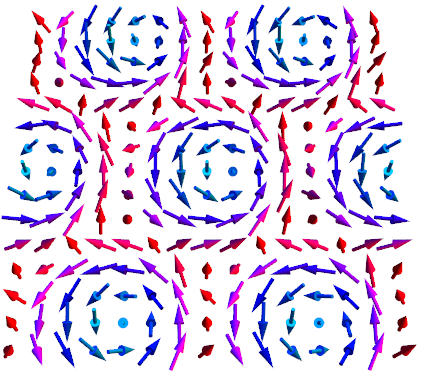
Figure 1: (Color online) Schematic illustration for spin order of skyrmion-crystal solution (left panel) and the corresponding distribution of energy density in zero magnetic field (right panel). The energy density is lower at the center of skyrmion because the local spin chirality is large there that is favored by DM interaction; it is larger in the boundaries of skyrmions but the spins there favor a perpendicular magnetic field.

Furthermore, we study what will happen if there exists a magnetic anisotropy in the system. Such an anisotropy can be introduced by adding the term $\sum_{j}\eta(S^{z}_{j})^{2}$ in the spin model (1) in which either the easy axis is chosen as $z$-axis or the easy plane as $x$-$y$ plane for $\eta<0$ or $\eta>0$, respectively. Choosing this kind of anisotropy is due to keeping the original rotational symmetry about the $z$-axis. Then the above gauge Landau-Lifshitz equation (5) turns to the following anisotropic one,

$$\frac{\partial}{\partial t}\bm{M}=a^{2}J\bm{M}\times D^{2}\bm{M}-2\eta\bm{M}\times\bm{M}^{\prime},$$ (10)

with $\bm{M}^{\prime}=(0,0,M_{z})$. Note that the gauge potential with skyrmion-crystal solution merely contributes an easy plane anisotropy. When the anisotropy coexist with the aforementioned gauge potential relevant to the skyrmion-crystal solution, the eigenequation for the original gauge Landau-Lifshitz equation in $k$-space is modified. One can choose the right-handed helical mode $\left(k_{y},-k_{x},i\rho\left|\bm{k}\right|\right)$ in which $\rho=\sqrt{\xi^{2}+1}-\xi$, where $\xi=\left(\gamma^{2}+2J\eta/a^{2}\right)/\left(4J\gamma\left|\bm{k}\right|\right)$. In real space, this mode is a helical order of elliptic contour with $\rho$ referring to ratio of semiminor and semimajor axes. It can be seen that the larger the $\eta$ is, the smaller the $\rho$ will be, which is in consistent with the requirement for minimizing the energy. When $\xi=0$ we have $\rho=1$, it occurs a cancelation between the added anisotropy term and the second order term of $\gamma$ arising from the gauge potential.

Now we turn to investigate finite temperature effects of our covariant model which contains DM interaction and magnetic anisotropy simultaneously. For convenience in numerical simulation, we start from the lattice version,

$$H= \sum_{\bm{r},\bm{e}}\Bigl{[}-J\bm{S}_{\bm{r}}\cdot\bm{S}_{\bm{r}+a\bm{e}}-K\bm{e}\cdot\left(\bm{S}_{\bm{r}}\times\bm{S}_{\bm{r}+a\bm{e}}\right)\Bigr{]}$$

$$+\sum_{\bm{r}}\Bigl{[}\frac{K^{2}}{2J}\left(S_{\bm{r}}^{z}\right)^{2}-BS_{\bm{r}}^{z}\Bigr{]},$$ (11)

where $\bm{S}$ denotes classical spin of unit module; $\bm{e}$ refers to $\hat{x}$ or $\hat{y}$ and $\bm{r}$ runs through the lattice site of the base space; $J$, $K$ and $B$ denote the exchange, the strength of DM interaction and the external magnetic field, respectively. In our numerical calculation, the Boltzmann constant $k_{B}$ and the lattice spacing $a$ is taken as unit. We do Monte Carlo simulations in various regimes of model parameters. For zero magnetic field $B=0$, we find, for a specific strength of DM interaction $K/J=\sqrt{2}\tan{(2\pi/6)}$, that the system goes from disordered phase to helical phase and then to a new phase when temperature is lowering. The new phase (see Fig. 2) presents a square lattice of alternatively placed skyrmion fragments, some of which appear to be imbedded among spin helical textures that is marked by black dot-lines in Fig. 2. Since the new phase appears in zero magnetic field, it is an emergence of spontaneous formation of skyrmion-fragment lattice. For weaker strength of DM interaction, saying $K/J=\sqrt{2}\tan{(2\pi/9)}$, we plot the phase diagrams in the plane of temperature versus magnetic field based on our Monte Carlo simulations for both our model (Unified Spin Order Theory via Gauge Landau-Lifshitz Equation) and the conventional model Tokura . Our results manifest that the landscape of those two phase diagrams are similar while the area ratio of skyrmion lattice phase to helical phase in our model is larger than that in the conventional model (see Fig. 3).

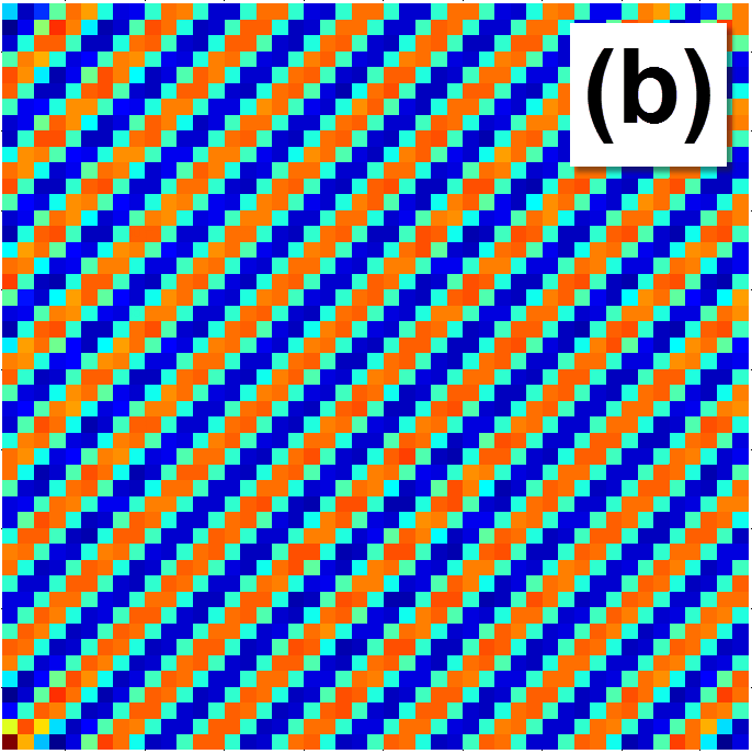
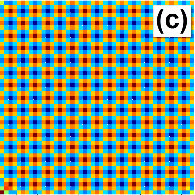
Figure 2: (Color online) (a) Spin order of skyrmion-fragment phase. Here is a patch of spin textures from our simulation for $K/J=\sqrt{2}\tan{(2\pi/6)}$. Along the black dot-line arrows the spins form a helical order where each two successive spins have relative $60^{\circ}$ difference in angle. (b) and (c) The spin $z$-$z$ correlation in the 48 by 48 lattice for various phases in zero magnetic field. Temperature is lowering, it goes from disordered to helical (b) then to skyrmion-fragment (c) phases.

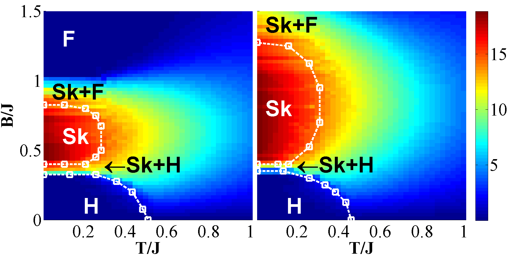
Figure 3: (Color online) Phase diagram of various spin orders (Sk means skyrmion lattice, H helical, F ferromagnetic, and $+$ coexistence) in the plane of magnetic field versus temperature calculated in the $36$ by $36$ lattice for DM model (left panel) and our covariant model (right panel). The color indicates the total number of skyrmions. The helical phase and ferromagnetic phase have no skyrmions and the skyrmion lattice phase have many skyrmions. The area ratio of skyrmion phase to helical phase is larger in our covariant model.

In conclusion, the gauge Landau-Lifshitz equation, as the continuum limit of the tilted SU(2) spin model, provides a unified description for various spin orders. The double periodic solution we found implies the conical spiral, in-plane spiral, helical, and ferromagnetic spin orders as special cases, respectively. The skyrmion-crystal order is a solution corresponding to a SO(3) gauge with nonvanishing strength tensor. As to the finite temperature behavior, a spontaneous formation of skyrmion-fragment lattice occurs in zero magnetic field, and the area ratio of skyrmion phase to helical phase is larger in our covariant model than in the conventional DM model. Note that the magnon band structure observed in recent experiments heliband does not contradict to double periodic dynamics since it happens when the system is described by a three-dimensional gauge potential $\bm{A}_{x}=\left(-\gamma/J,0,0\right)$, $\bm{A}_{y}=\left(0,-\gamma/J,0\right)$ and $\bm{A}_{z}=\left(0,0,-\gamma/J\right)$. This gauge potential is rotationally invariant and does not bring in anisotropy, so our model is equivalent to the conventional model and the ground state is the circularly helical state with wave vector $\gamma/J$.

We thank J.H. Han for useful communications. The work is supported by NSFCs (grant No.11074216 & No.11074218) and PCSIRT (Grant No. IRT0754).

References

- (1) M. Fiebig, J. Phys. D 38, R123 (2005).
- (2) Y. Tokura, Science 312, 1481 (2006).
- (3) W. Eerenstein, N. D. Mathur, and J. F. Scott, Nature 442, 759 (2006).
- (4) T. Choi, Y. Horibe, H. T. Yi, Y. J. Choi, Weida Wu, S.-W. Cheong, Nat. Mater. 9, 253 (2010).
- (5) H. Katsura, N. Nagaosa, and A. V. Balatsky, Phys. Rev. Lett. 95, 057205 (2005).
- (6) S. Mühlbauer, B. Binz, F. Jonietz, C. Pfleiderer, A. Rosch, A. Neubauer, R. Georgii, and P. Böni, Science 323, 915 (2009).
- (7) X. Z. Yu, Y. Onose, N. Kanazawa, J. H. Park, J. H. Han, Y. Matsui, N. Nagaosa, and Y. Tokura, Nature 465, 901 (2010).
- (8) M. Janoschek, F. Bernlochner, S. Dunsiger, C. Pfleiderer, P. Böni, B. Roessli, P. Link, and A. Rosch, Phys. Rev. B 81, 214436 (2010).
- (9) T. Kimura, S. Ishihara, H. Shintani, T. Arima, K. T. Takahashi, K. Ishizaka, and Y. Tokura, Phys. Rev. B 68, 060403(R) (2003).
- (10) I. Dzyaloshinsky, J. Phys. Chem. Solids 4, 241 (1958).
- (11) T. Moriya, Phys. Rev. 120, 91 (1960); Phys. Rev. Lett. 4, 228 (1960).
- (12) L. Shekhtman, O. Entin-Wohlman, and A. Aharony, Phys. Rev. Lett. 69, 836 (1992).
- (13) R. Gilmore, Lie Groups, Lie Algebra, and Some of Their Applications, (Dover Publications, New York 2005).
- (14) Y. Yamasaki, S. Miyasaka, Y. Kaneko, J.-P. He, T. Arima, and Y. Tokura, Phys. Rev. Lett. 96, 207204 (2006).
- (15) M. Kenzelmann, A. B. Harris, S. Jonas, C. Broholm, J. Schefer, S. B. Kim, C. L. Zhang, S.-W. Cheong, O. P. Vajk, and J. W. Lynn, Phys. Rev. Lett. 95, 087206 (2005).
- (16) M. Uchida, Y. Onose, Y. Matsui, and Y. Tokura, Science 311, 359 (2006).
- (17) T. H. R. Skyrme, Nucl. Phys. 31, 556 (1962).
- (18) J. H. Han, J. Zang, Z. Yang, J.-H. Park, and N. Nagaosa, Phys. Rev. B 82, 094429 (2010).