Symmetry Analysis for the Ruddlesden-Popper Systems, Ca₃Mn₂O₇ and Ca₃Ti₂O₇

Abstract

We perform a symmetry analysis of the zero-temperature instabilities of the tetragonal phase of Ca₃Mn₂O₇ and Ca₃Ti₂O₇ which is stable at high temperature. We introduce order parameters to characterize each of the possible lattice distortions in order to construct a Landau free energy which elucidates the proposed group-subgroup relations for structural transitions in these systems. We include the coupling between the unstable distortion modes and the macroscopic strain tensor. We also analyze the symmetry of the dominantly antiferromagnetic ordering which allows weak ferromagnetism. We show that in this phase the weak ferromagnetic moment and the spontaneous ferroelectric polarization are coupled, so that rotating one of these ordering by applying an external electric or magnetic field one can rotate the other ordering. We discuss the number of different domains (including phase domains) which exist in each of the phases and indicate how these may be observed.

I INTRODUCTION

Figure 1: (Color online) The unit cell of the RP ($n=2$) system (left) and the ($n=1$) system (right).

Ruddlesden-Popper (RP) systems [RP, ] are compounds of the form A_2+nB_1+nC_4+3n, where $n$ is an integer, and the valences of the ions are usually A $=+2$, B $=+4$ and C (oxygen) $=-2$. Systems like SrTiO₃ can be regarded as being $n=\infty$. At high temperatures $T\approx 800$K, their crystal structure is tetragonal, consisting of $n$-layer units, each layer consisting of vertex sharing oxygen octahedra at whose center sit a B ion, as shown in Fig. 1. (For an alternative illustration, see Ref. ARIAS, . As the temperature is lowered these systems can undergo structural phase transitions into orthorhombic structures.[STRUC1, ; STRUC2, ; STRUC3, ; STRUC4, ; STRUC5, ] These structural transitions usually involve reorientation of oxygen octahedra, a subject which has a long history,[ARIAS, ] of which the most relevant references for the present paper are those[STR1, ; STR2, ; STR3, ] which deal with the general symmetry aspects of these transitions. One reason for the continuing interest in octahedral reorientations is because they are important for many interesting electronic properties, such as high-$T_{c}$ superconductivity,[BM, ] colossal magnetoresistance,[CMR, ], metal-insulator transitions,[ARG, ] and magnetic ordering.[LOB, ]

Here we will focus on the $n=2$ RP systems, Ca₃Mn₂O₇ (CMO) and Ca₃Ti₂O₇ (CTO), which present less complex scenarios than the $n=1$ systems. It seems probable[STRUC5, ; LAB, ] that well above room temperature the crystal structure of CMO is that of the tetragonal space group I4/mmm, # 139 (space group numbering is that of Ref. ITC, ), and at room temperature that of space group Cmc2₁ (# 36).[GUIB, ] The theory of isotropy subgroups[UTAH, ] strongly forbids a direct transition from I4/mmm to Cmc2₁. In fact, first principles calculations on these systems by Benedek and Fennie (BF) [NATURE, ] and on other systems[PEREZ, ] indicate that the transition from I4/mmm to Cmc2₁ should proceed via an intermediate phase which is probably Cmcm (#63), consistent with Ref. UTAH, . Up to now no such intermediate phase has been observed for CMO or CTO. Unlike the other phases, the Cmc2₁ phase does not possess a center of inversion symmetry and is allowed to have a spontaneous polarization. Recent measurements on ceramic Ca₃Mn₂O₇ find a clear pyroelectric signal consistent with the onset of ferroelectric order close to $T^{*}=280$K.[LAWES, ] Therefore $T^{*}$ is identified as the temperature at which Cmc2₁ appears. Since this ferroelectric transition seems to be a continuous and well-developed one and since a direct continuous transition between I4/mmm and Cmc2₁ is inconsistent with Landau theory,[UTAH, ] the seemingly inescapable conclusion is that the phase for $T$ slightly greater than $T^{*}$ is not I4/mmm, but is some other phase which does not allow a spontaneous polarization. Thus the phase at temperature just above $T=280$K may be the long sought for Cmcm phase. In fact, the Cmcm phase has been observed in the isostructural compounds LaCa₂Mn₂O₇[GREEN, ] and Bi_0.44Ca_2.56Mn₂O₇[QIN, ] at room temperature. In view of the results of Refs. STRUC5, and LAB, , it is possible that the Cmcm phase may exist only over a narrow range of temperature. As the temperature is further lowered, an antiferromagnetic phase is observed.[JUNG, ; LOB, ] In this phase, which appears at $T=115$K,[LOB, ] the antiferromagnetic order is accompanied by weak ferromagnetism.[JUNG, ; LOB, ]

Theoretically, there have been efforts to understand systems like these from first principles calculations. For instance, Ref. WHANG, found the nearest neighbor exchange $J_{\rm nn}$ within a bilayer to be $J_{\rm nn}/k_{\rm B}=-39$K, giving a Curie-Weiss $\Theta=-244$K, whereas Ref. CARDOSO, found $J_{\rm nn}/k_{\rm B}=200$K. The former calculation agrees much better with experiment[FAW, ] which gave $\theta=-465$K. Both groups studied the electronic band structure but it was not entirely clear what space group their calculations predicted. More detailed information on the symmetry of the structures comes from the first principles calculations of BF some of which included spin-orbit interactions. These calculations give a weak ferromagnetism of $0.18\mu_{\rm B}$ per unit cell which is somewhat smaller than $0.3\mu_{\rm B}$ per spin.[FOOT, ] However, inclusion of spin-orbit interactions enabled BF to obtain the correct symmetry of the magnetoelectric behavior. Here we discuss in detail the symmetry properties of the various phases and experimental consequences such as the interactions between various order parameters (OP’s) and the number and symmetry of the various domains which may be observed. Several of these issues were discussed by BF, but a more complete and systematic analysis is given here.

Our approach to symmetry is similar to that of Ref. PEREZ, in connection with the Aurivillius compound SrBi₂Ta₂O₉ (SBTO): we adopt the high-temperature tetragonal structure as the “reference” structure and analyze the instabilities at zero temperature which lead to the lower temperature phases. Although CMO and CTO do differ from SBTO, their crystal symmetry is the same as SBTO and hence many of the results we find here are similar to those for SBTO. Here we emphasize some of the experimental consequences of the symmetries we find (such as the enumeration of the different possible structurally ordered domains) and also we explore the nature of the macroscopic strains, the ferroelectric polarization, the magnetic ordering, and the coupling between structural distortions and these degrees of freedom.

Briefly, this paper is organized as follows. In Sec. II we outline the basic approach used to analyze the symmetry of the systems in question. In Sec. III we give a symmetry analysis of the resulting phases which result from the structural instabilities found by BF. This analysis closely parallels that of Perez-Mato et al.[PEREZ, ]. In Sec. IV we discuss the second structural transition in which the other two irreps condense to reach the Cmc2₁ phase. In Sec. V we discuss the symmetry of the magnetic ordering. We also explore the coupling betweeen the distortions and the strains, the polarization, and the magnetic ordering. Throughout the paper we point out experiments which are needed in order to remove crucial gaps in our understanding of the structural phase diagram of these systems. In Sec. VI we enumerate the possible domains that can occur and briefly discuss their dynamics. Our conclusions are summarized in Sec. VII.

II SYMMETRY ANALYSIS

Our symmetry analysis will be performed relative to the tetragonal I4/mmm structure which is stable at high temperatures. In this high-temperature reference structure one has atoms at their equilibrium positions ${\bf R}^{(0)}({\bf n},\tau)$, where

$$R_{\alpha}^{(0)}(n_{1},n_{2},n_{3};\tau) \equiv n_{1}R_{1,\alpha}+n_{2}R_{2,\alpha}+n_{3}R_{3,\alpha}+\tau_{\alpha}\ ,$$

where the lattice vectors are

$${\bf R}_{1} \equiv (-1/2,1/2,1/2)\ ,\ \ \ \ {\bf R}_{2}\equiv(1/2,-1/2,1/2)\ ,$$

$${\bf R}_{3} \equiv (1/2,1/2,-1/2)\ ,$$

where $\alpha$ labels Cartesian components, real space coordinates are expressed as fractions of lattice constants (so that, for instance, ${\bf R}_{1}$ denotes $(-a/2,a/2,c/2)$), and the number $\tau$ labels sites within the unit cell at the position vector $\tau$, as listed in Table 1. The associated tetragonal reciprocal lattice vectors are

$${\bf G_{1}} = (0,1,1)\ ,\ \ \ {\bf G_{2}}=(1,0,1)\ ,\ \ \ {\bf G_{3}}=(1,1,0)\ ,$$

in reciprocal lattice units so that, for instance, ${\bf G_{1}}$ denotes $2\pi(0,1/a,1/c)$.

Figure 2: (Color online) The group-subgroup structure arising from the first principles calculations. The transitions from I4/mmm are labeled with irrep that is condensing. In the final transition to Cmc2₁ we show below that the two remaining irreps condense to that all three irreps have condensed to form Cmc2₁. This diagram does not deal with magnetic ordering.

This work was stimulated by the first principles calculations of BF on the instabilities at zero temperature of the reference tetragonal system. For CMO the instabilities at zero temperature occur for the irreps $X_{3}^{-}$ and $X_{2}^{+}$ at the zone boundary $X$ points which are ${\bf K}=(1/2,1/2,0)\equiv{\bf q}_{1}$ and ${\bf K}=(1/2,-1/2,0)\equiv{\bf q}_{2}$. (The superscript indicates the parity under inversion about the origin.) Since $-{\bf q}_{n}$ is equal (modulo a reciprocal lattice vector) to ${\bf q}_{n}$, the vectors ${\bf q}_{1}$ and ${\bf q}_{2}$ exhaust the star of $X$. Also a zone center phonon of the two dimensional irrep $\Gamma_{5}^{-}$ is nearly unstable. These results suggest the group-subgroup structure shown in Fig. 2, which is similar to that for SBTO.[PEREZ, ] We therefore consider structures having distorted positions given by

$$R_{\alpha}({\bf n},\tau) = R_{\alpha}^{(0)}({\bf n},\tau)+u_{\alpha}(\tau)e^{i{\bf q}\cdot(\sum_{k}{\bf R}_{k}n_{k})}$$

$$\ +\sum_{\beta}e_{\alpha\beta}R_{\beta}^{(0)}({\bf n},\tau)\ ,$$

where ${\bf q}$ is the wave vector of the distortion mode, ${\bf u}(\tau)$ is the distortion taken from Table 1, and $\epsilon_{\alpha\beta}$ is the macroscopic strain tensor. The leading terms in the Landau expansion of the free energy of the distorted structure relative to the reference tetragonal structure will have terms quadratic in the strains $e_{\alpha\beta}$ and the microscopic displacements ${\bf u}(\tau)$ within the unit cell. The fact that the free energy has to be invariant under all the symmetry operations of the “vacuum” (i. e. the reference tetragonal structure) restricts the microscopic displacements to be a linear combination of the basis vectors of the irrep in question. The basis functions are listed in Table 1 and the representation matrices for the generators of the irreps are given in Table 2[FN1, ] in terms of the Pauli matrices

$${\mbox{\boldmath{$\sigma$}}}_{x} = \left[\begin{array}[]{cc}0&1\\ 1&0\\ \end{array}\right]\hskip 14.45377pt{\mbox{\boldmath{$\sigma$}}}_{y}=\left[\begin{array}[]{cc}0&-i\\ i&0\\ \end{array}\right]\hskip 14.45377pt{\mbox{\boldmath{$\sigma$}}}_{z}=\left[\begin{array}[]{cc}1&0\\ 0&-1\\ \end{array}\right]\ .$$ (7)

Table 1: Basis functions $\Psi_{1}^{(Z)}({\bf R},\tau)=\Psi^{(Z)}_{1,n}(\tau)\cos({\bf q}\cdot{\bf R})$ and $\Psi_{2}^{(Z)}({\bf R},\tau)=\Psi^{(Z)}_{2,n}(\tau)\cos({\bf q}\cdot{\bf R})$ for the distortion vector under irrep $Z$, where $Z=5,3,2$ indicates irrep $\Gamma_{5}^{-}$, $X_{3}^{-}$, and $X_{2}^{+}$, respectively, and $n=x,y,z$ labels the components. The $\Psi$’s are normalized according to Eq. (15). For the $X$ irreps the wave vector of $\Psi_{k,n}^{(X)}({\bf R},\tau)$ is ${\bf q}_{k}$. For $\Gamma_{5}^{-}$ the wave vector is ${\bf q}=0$. For each site $\tau$ we give the three components ($n=1,2,3)$ of the vector displacement. The values of the displacements in this table are not restricted by symmetry. The values of the structure parameters for CMO, taken from Ref. STRUC5, , are $\rho=0.311$, $\xi=0.100$, $\chi=0.205$, and $\tau=0.087$.

$\tau$	$\tau$	$\Psi_{1,n}^{(5)}(\tau)$			$\Psi_{2,n}^{(5)}(\tau)$			$\Psi_{1,n}^{(3)}(\tau)$			$\Psi_{2,n}^{(3)}(\tau)$			$\Psi_{1,n}^{(2)}(\tau)$			$\Psi_{2,n}^{(2)}(\tau)$
A sites
1	$(0,0,\rho+1/2)$	$u$	0	0	0	$u$	0	$a$	$-a$	0	$-a$	$-a$	0	0	0	0	0	0	0
2	$(0,0,-\rho+1/2)$	$u$	0	0	0	$u$	0	$a$	$-a$	0	$-a$	$-a$	0	0	0	0	0	0	0
3	$(0,0,1/2)$	$v$	0	0	0	$v$	0	$b$	$-b$	0	$-b$	$-b$	0	0	0	0	0	0	0
B sites
4	$(0,0,\xi)$	$w$	0	0	0	$w$	0	$c$	$-c$	0	$-c$	$-c$	0	0	0	0	0	0	0
5	$(0,0,-\xi)$	$w$	0	0	0	$w$	0	$c$	$-c$	0	$-c$	$-c$	0	0	0	0	0	0	0
O sites
6	$(0,0,0)$	$x$	0	0	0	$x$	0	$d$	$-d$	0	$-d$	$-d$	0	0	0	0	0	0	0
7	$(0,0,\chi)$	$y$	0	0	0	$y$	0	$e$	$-e$	0	$-e$	$-e$	0	0	0	0	0	0	0
8	$(0,0,-\chi)$	$y$	0	0	0	$y$	0	$e$	$-e$	0	$-e$	$-e$	0	0	0	0	0	0	0
9	$(0,1/2,\tau)$	$z_{1}$	0	0	0	$z_{2}$	0	$0$	$0$	$f$	$0$	$0$	$f$	$-h$	$-g$	0	$-h$	$g$	0
10	$(0,1/2,-\tau)$	$z_{1}$	0	0	0	$z_{2}$	0	$0$	$0$	$-f$	$0$	$0$	$-f$	$-h$	$-g$	0	$-h$	$g$	0
11	$(1/2,0,\tau)$	$z_{2}$	0	0	0	$z_{1}$	0	$0$	$0$	$-f$	$0$	$0$	$f$	$g$	$h$	0	$-g$	$h$	0
12	$(1/2,0,-\tau)$	$z_{2}$	0	0	0	$z_{1}$	0	$0$	$0$	$f$	$0$	$0$	$-f$	$g$	$h$	0	$-g$	$h$	0

Table 2: Representation matrices $M^{(3)}$, $M^{(2)}$, and $M^{(5)}$ for the generators of the irreps $X_{3}^{-}$, $X_{2}^{+}$, and $\Gamma_{5}^{-}$, respectively. Here ${\bf r}^{\prime}={\cal O}{\bf r}$ and the $\sigma$’s are the Pauli matrices. These matrices are related to those of Ref. UTAH, [UTAH2, ] by a unitary transformation which, for $\Gamma_{5}^{-}$ takes $({\mbox{\boldmath{$\sigma$}}}_{x},{\mbox{\boldmath{$\sigma$}}}_{y},{\mbox{\boldmath{$\sigma$}}}_{z})$ into $(-{\mbox{\boldmath{$\sigma$}}}_{x},-{\mbox{\boldmath{$\sigma$}}}_{y},{\mbox{\boldmath{$\sigma$}}}_{z})$. For $X_{2}^{+}$ and $X_{3}^{-}$ the unitary transformation takes (${\mbox{\boldmath{$\sigma$}}}_{x},{\mbox{\boldmath{$\sigma$}}}_{y},{\mbox{\boldmath{$\sigma$}}}_{z})$ into $(-{\mbox{\boldmath{$\sigma$}}}_{z},{\mbox{\boldmath{$\sigma$}}}_{y},-{\mbox{\boldmath{$\sigma$}}}_{x})$. Unlike Ref. UTAH, we choose a representation in which the matrices representing the translations ${\bf T}_{n}$ are diagonal.

${\cal O}=$	${\cal R}_{4}$	$m_{d}$	$m_{z}$	${\bf T}_{1}$	${\bf T}_{2}$	${\bf T}_{3}$
${\bf r}^{\prime}=$	$(\overline{y},x,z)$	$(y,x,z)$	$(x,y,\overline{z})$	$(x+1,y,z)$	$(x,y+1,z)$	$(x+\frac{1}{2},y+\frac{1}{2},z-\frac{1}{2})$
${\bf M}^{(3)}({\cal O})=$	$-i{\mbox{\boldmath{$\sigma$}}}_{y}$	$-{\mbox{\boldmath{$\sigma$}}}_{z}$	${\bf 1}$	$-{\bf 1}$	$-{\bf 1}$	$-{\mbox{\boldmath{$\sigma$}}}_{z}$
${\bf M}^{(2)}({\cal O})=$	${\mbox{\boldmath{$\sigma$}}}_{x}$	$-{\bf 1}$	${\bf 1}$	$-{\bf 1}$	$-{\bf 1}$	$-{\mbox{\boldmath{$\sigma$}}}_{z}$
${\bf M}^{(5)}({\cal O})=$	$i{\mbox{\boldmath{$\sigma$}}}_{y}$	${\mbox{\boldmath{$\sigma$}}}_{x}$	${\bf 1}$	${\bf 1}$	${\bf 1}$	${\bf 1}$

Using the basis functions $\Psi_{1}^{(Z)}$ and $\Psi_{2}^{(Z)}$ listed in Table 1 one can check that the matrices of Table 2 do form a representation, so that for an operator ${\cal O}$ we have

$${\cal O}\left[\begin{array}[]{c}\Psi_{1}^{(Z)}\\ \Psi_{2}^{(Z)}\\ \end{array}\right]=\left[\begin{array}[]{c c }M_{11}({\cal O})&M_{12}({\cal O})\\ M_{21}({\cal O})&M_{22}({\cal O})\\ \end{array}\right]\left[\begin{array}[]{c}\Psi_{1}^{(Z)}\\ \Psi_{2}^{(Z)}\\ \end{array}\right]\ ,$$ (14)

where the $\Psi$’s are normalized:

$$\sum_{n\tau}\Psi^{(Z)}_{k,n}(\tau)^{2}=1{\AA}^{2}\ .$$ (15)

We now introduce OP’s $Q_{1}^{(Z)}$ and $Q_{2}^{(Z)}$ as amplitudes of these normalized distortions, so that a distortion $\Phi_{Z}$ of the irrep Z can be written as $\Phi_{Z}=Q_{1}^{(Z)}\Psi_{1}^{(Z)}+Q_{2}^{(Z)}\Psi_{2}^{(Z)}$ and

$${\cal O}\Phi_{Z} \equiv {\cal O}[Q_{1}^{(Z)}\Psi_{1}^{(Z)}+Q_{2}^{(Z)}\Psi_{2}^{(Z)}]$$

$$= [M_{11}^{(Z)}({\cal O})Q_{1}^{(Z)}+M_{21}^{(Z)}({\cal O})Q_{2}^{(Z)}]\Psi_{1}^{(Z)}$$

$$+[M_{12}^{(Z)}({\cal O})Q_{1}^{(Z)}+M_{22}^{(Z)}({\cal O})Q_{2}^{(Z)}]\Psi_{2}^{(Z)}\ .$$

We now interpret this as defining how the order parameters transform when the $\Psi_{n}^{(Z)}$ are regarded as fixed. Thus we have

$${\cal O}\left[\begin{array}[]{c}Q_{1}^{(Z)}\\ Q_{2}^{(Z)}\end{array}\right] = \left[\begin{array}[]{cc}M_{11}^{(Z)}({\cal O})&M_{21}^{(Z)}({\cal O})\\ M_{12}^{(Z)}({\cal O})&M_{22}^{(Z)}({\cal O})\\ \end{array}\right]\left[\begin{array}[]{c}Q_{1}^{(Z)}\\ Q_{2}^{(Z)}\\ \end{array}\right]\ .$$ (22)

Note that the OP’s transform according to the transpose of the irrep matrices.

III Unstable Irreps

III.1 $X_{3}^{-}$

The irrep $X_{3}^{-}$ of the little group (of the wave vector) is one dimensional. However, since there are two wave vectors in the star of $X$, we will follow Ref. UTAH, and construct the two dimensional irrep which incorporates both wave vectors in the star of ${\bf X}$. The resulting two dimensional matrices are given in Table 2. From the basis functions for irrep $X_{3}^{-}$ given in Table 1, one sees that the distortion can describe the alternating tilting of the oxygen octahedra about a $(1,\overline{1},0)$ direction if ${\bf q}={\bf q}_{1}$ and about a $(1,1,0)$ direction if ${\bf q}={\bf q}_{2}$, as shown in Fig. 3. We now construct the form of the free energy when the distortion is given by[FNA, ]

$$\Phi = Q_{3}^{-}({\bf q}_{1})\Psi_{1}^{(3)}+Q_{3}^{-}({\bf q}_{2})\Psi_{2}^{(3)}\ .$$

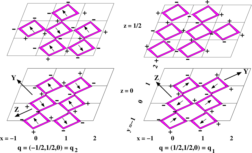
Figure 3: (Color online) Schematic diagram of the displacements $\Psi^{(3)}_{1}({\bf R},\tau)$, left and $\Psi^{(3)}_{2}({\bf R},\tau)$, right of the oxygen octahedra. All coordinates are in the parent tetragonal system. The arrows represent displacements within the $x$-$y$ plane and the $+$ and $-$ signs, displacements collinear with the $z$-axis. The arrows represent the displacement of the apical oxygen at $(0,0,\chi)$, which is the same as that at $(0,0,-\chi)$. The displacement of the shared apical oxygen at $(0,0,0)$ is not shown. The algebraic sign of the displacements in the $z$ direction of the equatorial oxygen at $(x,y,\tau)$ in the unit cell is indicated. The displacement of the oxygen at $(x,y,-\tau)$ is the negative of that at $(x,y,\tau)$. The orthorhombic axes for Cmcm are $X$, $Y$, and $Z$. The distortion of left panel is obtained from that of the right panel by a 90^o rotation about the positive $z$-axis.

To construct the form of the free energy for this structure, note that wave vector conservation requires that the free energy be a function of $Q_{3}({\bf q}_{1})^{2}$ and $Q_{3}({\bf q}_{2})^{2}$ because $2{\bf q}_{1}$ and $2{\bf q}_{2}$ are reciprocal lattice vectors but ${\bf q}_{1}+{\bf q}_{2}$ is not a reciprocal lattice vector. Then, using the irrep matrices given in Table 2, one can check that the free energy in terms of the $X_{3}^{-}$ OP’s must be of the form

$${\cal F}({\bf X}_{3}) = \frac{a}{2}(T-T_{3})[Q_{3}({\bf q}_{1})^{2}+Q_{3}({\bf q}_{2})^{2}]$$ (23)

$$\ +\frac{1}{4}u[Q_{3}({\bf q}_{1})^{2}+Q_{3}({\bf q}_{2})^{2}]^{2}$$

$$\ +v[Q_{3}({\bf q}_{1})Q_{3}({\bf q}_{2})]^{2}+{\cal O}(Q^{6})\ ,$$

where $a>0$ and $T_{3}$ is the temperature at which this irrep becomes active if it is the only relevant OP). The first principles calculations of BF indicate that $u>0$. To treat the coupling between the $Q$’s and the strains we consider the strain-dependent contribution to the free energy $F_{Q\epsilon}$. The term whereby the $Q$’s induce a strain is linear in the strain and thus we write $F_{Q\epsilon}$ as

$$F_{Q\epsilon} = \frac{1}{2}\sum_{nm}c_{nm}\epsilon_{n}\epsilon_{m}+\sum_{klm}\gamma_{klm}\epsilon_{kl}Q_{3}^{-}({\bf q}_{m})^{2}$$

$$\equiv \frac{1}{2}\sum_{nm}c_{nm}\epsilon_{n}\epsilon_{m}+V_{Q\epsilon}\ ,$$

where the first term is in Voigt[VOIGT, ] notation, where $1\equiv x,x$, etc. and only $c_{11}$, $c_{12}$, $c_{13}$, $c_{33}$, $c_{44}$, and $c_{66}$ are nonzero under tetragonal symmetry and

$$V_{Q,\epsilon} = \alpha\epsilon_{xy}[Q_{3}^{-}({\bf q}_{1})^{2}-Q_{3}^{-}({\bf q}_{2})^{2}]+[\beta(\epsilon_{xx}+\epsilon_{yy})$$ (24)

$$\ +\gamma\epsilon_{zz}][Q_{3}^{-}({\bf q}_{1})^{2}+Q_{3}^{-}({\bf q}_{2})^{2}]\ ,$$

where $\alpha$, $\beta$, and $\gamma$ (and similarly below) are arbitrary constants. The sign of the shear deformation $\epsilon_{xy}$ depends on the sign of $Q_{3}^{-}({\bf q}_{1})^{2}-Q_{3}^{-}({\bf q}_{2})^{2}$, a result similar to that given in Ref. AXE, .

As the temperature is reduced through the value $T_{3}$, a distortion of symmetry $X_{3}^{-}$ appears. For $v>0$ either one, but not both, of $Q_{3}({\bf q}_{1})$ and $Q_{3}({\bf q}_{2})$ are nonzero, so that $\epsilon_{xy}\not=0$ and a detailed analysis shows that the resulting structure is Cmcm (#63). The first principles calculations of BF imply that $v>0$, so, as indicated by Fig. 2, this possibility is the one realized for the RP systems we have studied. If $v$ had been negative, then we would have had a “double-${\bf q}$” state (i. e. a state simultaneously having two wave vectors) with $|Q_{3}({\bf q}_{1})|=|Q_{3}({\bf q}_{2})|$, so that $\epsilon_{xy}=0$ and the distorted structure would be the tetragonal space group P4₂/mnm (#136). These two space groups are listed in Ref. UTAH, as possible subgroups of I4/mmm which can arise out of the irrep $X_{3}^{-}$. These directions in OP-space [$Q_{3}({\bf q}_{1})-Q_{3}({\bf q}_{2})$-space] are stable with respect to perturbations due to higher order terms in Eq. (23) which are anisotropic in OP-space as long as $T$ is close enough to $T_{3}$ so that these perturbations are sufficiently small. We note that Ref. UTAH, lists Pnnm (#58) as an additional possible subgroup. This subgroup would arise if $v$ were exactly zero, in which case, even for $T$ arbitrarily close to $T_{3}$, the OP’s would be determined by higher order terms in Eq. (23) and would then not be restricted to lie along a high symmetry direction in OP space. However, to realize this possibility requires the accidental vanishing of the coefficient $v$ and the analogous sixth order anisotropy. This possibility should be rejected unless additional control parameters, such as the pressure or an electric field, are introduced which allow access to such a multicritical point.[STR3, ] As of this writing, the Cmcm phase (or any other phase intermediate between I4/mmm and Cmc2₁) has not been observed, although it has been observed in the isostructural systems LaCa₂Mn₂O₇[GREEN, ] and Bi_0.44Ca_2.56Mn₂O₇[QIN, ]

For future reference, it is convenient to introduce orthorhombic axes, so we arbitrary define them as in Fig. 4. If we condense $Q_{3}({\bf q}_{1})$, the tilting is about $Y$, the tetragonal [1 $\overline{1}$ 0] direction, whereas if we condense $Q_{3}({\bf q}_{2})$, the tilting is about $Z$, the tetragonal [1 1 0] direction. The sign of the OP indicates the sign of the tilting angle. Note that there are four domains of ordering, depending on which wave vector has condensed and the signs of the OP. These correspond to the four equivalent initial orientations of the tetragonal sample. In Ni₃V₂O₈, such a domain structure for two coexisting OP’s was confirmed experimentally,[DOMAIN, ] and it would be nice to do the same here. In Sec. VI we give a more detailed discussions of domains. Here we note that changing the sign of the OP $Q_{3}({\bf q}_{1})$ is equivalent to a unit translation along $\hat{x}$ or $\hat{y}$. Thus, as for an antiferromagnet, the phase of the order parameter within a single domain has no macroscopic consequences.

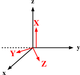
Figure 4: (Color online) The tetragonal axes (lower case) and the axes (capitals) we use to describe the orthorhombic phases.

Since the Cmcm structure has a center of inversion symmetry, it can not have a nonzero spontaneous polarization and an interaction $V_{Q,{\bf P}}$ which is linear in the polarization does not arise. It may seem mysterious that when we introduce a distortion which is odd under inversion, we still have a structure which is even under inversion. The point is that the distortion due to $X_{3}^{-}$ is odd under inversion about the origin, but is even under inversion with respect to $(1/2,0,0)$, about which point the parent tetragonal structure also has a center of inversion symmetry. To see the inversion symmetry of the distortion about $(1/2,0,0)$ from Fig. 3, note that inversion displaces the arrows and reverses their direction. Since a plus sign represents a positive $z$ distortion at $z=\tau$ and a negative $z$ distortion at $z=-\tau$, inversion takes a plus into a plus and a minus into a minus.

III.2 $X_{2}^{+}$

As in the case of $X_{3}^{-}$ we construct the two dimensional irrep which incorporates both wave vectors in the star of ${\bf X}$, whose matrices are given in Table 2. The allowed basis functions are given in Table 1 and are represented in Fig. 5. Once the configuration for one wave vector is determined, that of the other wave vector follows from a $90^{\rm o}$ rotation about the $z$-axis. So these are two different configurations (one for each $X$ wave vector) which have the same free energy. These two configurations differ in their stacking (which takes point ${\bf O}$ into point ${\bf O}^{\prime}$). This stacking degeneracy means that this transition takes the I4/mmm structure into one of two different settings of the space group which we identify below as Cmca. One sees that in this distortion the oxygen octahedra are rotated about the crystal $c$ axis as if they were interlocking gears. Notice that in the left panel of Fig. 5 all the clockwise turning octahedra have $r_{x}>r_{y}$ and all the counterclockwise ones have $r_{x}<r_{y}$, whereas in the right panel the clockwise turning octahedra have $r_{y}>r_{x}$ and the counterclockwise ones have $r_{y}<r_{x}$, where $r_{x}$ is the radius of the elliptically distorted octahedra along $x$ (or nearly $x$) and $r_{y}$ is the radius along $y$. Symmetry does not fix the sign of the radial distortion. Changing the sign of the radial distortion would lead to a different (inequivalent) structure in which the sign of all the radial arrows for both wave vectors would be changed. It would be interesting to observe this radial distortion in either (or both) calculations and experiment.

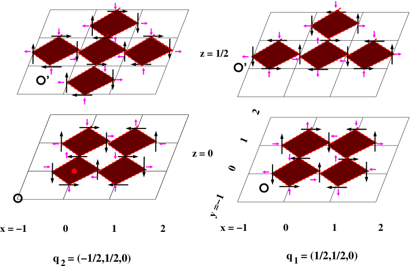
Figure 5: (Color online) Schematic diagram of the displacements for $X_{2}^{+}$, which are confined to the $x$-$y$ plane. All coordinates are in the parent tetragonal system. The large black arrows give the rotational distortion. The much smaller anisotropic radial distortion (which is allowed in $X_{2}^{+}$) is shown in magenta. In both panels the distortions are shown for sites in the planes $z=\pm\tau$ and $z=1/2\pm\tau$. The distortion is an even function of $\tau$. The distortion of the right panel is obtained from that of the left panel by a 90^o rotation about the $z$-axis. The translation vectors in the $x$-$y$ plane are $(1,1,0)$ and $(1,-1,0)$. In the left panel the translation vector $\Delta{\bf r}$ (which takes O into O’ and obeys $\exp(i{\bf q}\cdot\Delta{\bf r})=1$) is $(1/2,1/2,1/2)$ and in the right panel it is $(-1/2,1/2,1/2)$. These two wave vectors thus give rise to the two settings of the side-centered orthorhombic lattice.

As before, we introduce OP’s $Q_{2}({\bf q}_{1})$ and $Q_{2}({\bf q}_{2})$ by considering the free energy for which the distortion from tetragonal is given by $Q_{2}({\bf q}_{1})$ times the distortion for ${\bf q_{1}}$ plus $Q_{2}({\bf q}_{2})$ times the distortion for ${\bf q}_{2}$. As in Eq. (22), the transformation properties of these OP’s are determined by the matrices of Table 2. As before, wave vector conservation requires that the free energy be a function of $Q_{2}({\bf q}_{1})^{2}$ and $Q_{2}({\bf q}_{2})^{2}$. Using the transformation properties of the OP’s, we find that

$${\cal F}({\bf X}_{2}) = \frac{a^{\prime}}{2}(T-T_{2})[Q_{2}({\bf q}_{1})^{2}+Q_{2}({\bf q}_{2})^{2}]$$

$$\ +\frac{1}{4}u^{\prime}[Q_{2}({\bf q}_{1})^{2}+Q_{2}({\bf q}_{2})^{2}]^{2}$$

$$\ +v^{\prime}[Q_{2}({\bf q}_{1})Q_{2}({\bf q}_{2})]^{2}+{\cal O}(Q^{6})\ ,$$

where $a^{\prime}>0$, $u^{\prime}>0$, and $T_{2}$ is the temperature at which this irrep would become active, if it were the only relevant irrep. The free energy of the coupling to strains is

$$V_{Q,\epsilon} = \alpha^{\prime}\epsilon_{xy}[Q_{2}({\bf q}_{1})^{2}-Q_{2}({\bf q}_{2})^{2}]+[\beta^{\prime}(\epsilon_{xx}+\epsilon_{yy})$$

$$\ +\gamma^{\prime}\epsilon_{zz}][Q_{2}({\bf q}_{1})^{2}+Q_{2}({\bf q}_{2})^{2}]\ ,$$

where $\alpha^{\prime}$, $\beta^{\prime}$, and $\gamma^{\prime}$ are arbitrary coefficients. The coupling to the shear strain is allowed because both $\epsilon_{yx}$ and $Q_{2}({\bf q}_{1})^{2}-Q_{2}({\bf q}_{2})^{2}$ are odd under ${\cal R}_{4}$ and even under $m_{d}$. The term $[\epsilon_{xx}-\epsilon_{yy}][Q_{2}({\bf q}_{1})^{2}-Q_{2}({\bf q}_{2})^{2}]$ is not allowed because it is not invariant under $m_{d}$. Since this structure is even under inversion it can not have a spontaneous polarization, so $F_{Q,{\bf P}}$, the interaction linear in the polarization is zero.

Now we discuss the phases which Landau theory predicts. If $v^{\prime}>0$, then either $Q_{2}({\bf q}_{1})=0$ or $Q_{2}({\bf q}_{2})=0$, so that $\epsilon_{xy}\not=0$ and a detailed analysis shows that the resulting structure is Cmca (#64). Similarly, if $v^{\prime}<0$, then one has a double-${\bf q}$ state with $|Q_{2}({\bf q}_{1})|=|Q_{2}({\bf q}_{2})|$, the orthorhombic distortion vanishes, and we have the structure P4/mbm (#127). The other possibility listed in Ref. UTAH, is Pbnm (#35). As before, we ignore this possibility because it requires the accidental vanishing of $v^{\prime}$. The first principles calculations of BF indicate that $v^{\prime}>0$ as required by Fig. 2.

III.3 $\Gamma_{5}^{-}$

The allowed distortion of the two-dimensional irrep $\Gamma_{5}^{-}$ is given by the basis functions of Table 1 and this distortion breaks inversion symmetry. As before, we assume that the distortion $\Psi$ from I4/mmm is given by $Q_{5,1}$ times the distortion $\Psi_{1}^{(5)}$ plus $Q_{5,2}$ times the distortion for $\Psi_{2}^{(5)}$, where the $\Psi$’s are given in Table 1 and are seen to transform simlarly to $x$ or $y$. It follows that the OP’s $Q_{5,1}$ and $Q_{5,2}$, transform as $x$ and $y$, respectively. So under tetragonal symmetry the expansion of the free energy $F$ of the distortion $\Psi$ in powers of $Q_{5,1}$ and $Q_{5,2}$ assumes the form

$${\cal F}(\Gamma_{5}) = \frac{a^{\prime\prime}}{2}(T-T_{5})(Q_{5,1}^{2}+Q_{5,2}^{2})+\frac{1}{4}u^{\prime\prime}(Q_{5,1}^{2}+Q_{5,2}^{2})^{2}$$ (25)

$$\ +v^{\prime\prime}Q_{5,1}^{2}Q_{5,2}^{2}+{\cal O}(Q^{6})\ ,$$

where $a^{\prime\prime}>0$, $u^{\prime\prime}>0$, and $T_{5}$ is the temperature at which irrep $\Gamma_{5}$ becomes active (if it were the only relevant irrep). Since BF find that $\Gamma_{5}^{-}$ is not actually unstable for CMO, $T_{5}<0$. Using the fact (see Tables 1 or 2) that $Q_{5,1}$ and $Q_{5,2}$ transform like $x$ and $y$, we see that

$$V_{Q\epsilon} = \alpha\epsilon_{zz}(Q_{5,1}^{2}+Q_{5,2}^{2})+\beta(\epsilon_{xx}+\epsilon_{yy})(Q_{5,1}^{2}+Q_{5,2}^{2})$$ (26)

$$\ +\gamma(\epsilon_{xx}-\epsilon_{yy})(Q_{5,1}^{2}-Q_{5,2}^{2})+\delta\epsilon_{xy}Q_{5,1}Q_{5,2}\ .$$

Because this phase is not centrosymmetric, it can support a nonzero spontaneous polarization. This will be discussed in a later subsection.

The free energy of Eq. (25) gives rise to two principal scenarios. If $v^{\prime\prime}>0$, then either $Q_{5,1}$ or $Q_{5,2}$ (but not both) condense at $T_{5}$. Then Eq. (26) indicates that $\epsilon_{xy}=0$ and $\epsilon_{xx}\not=\epsilon_{yy}$ and a detailed analysis of the distortions indicates that we condense into space group Imm2 (#44). Alternatively, if $v^{\prime\prime}<0$ then Eq. (25) indicates that $|Q_{5,1}|=|Q_{5,2}|$. Equation (26) implies that $\epsilon_{xy}\not=0$ and $\epsilon_{xx}=\epsilon_{yy}$ and we condense into space group F2mm (#42). As before, these distorted space groups agree with the results in Ref. UTAH, . However, an additional subgroup is listed as realizable from this irrep, namely Cm (#8). As before, to realize this possibility requires the accidental vanishing of $v^{\prime\prime}$, a possibility we reject. The first principles calculations of BF imply that $v^{\prime\prime}<0$ so that space group F2mm would be realized if $\Gamma_{5}^{-}$ were to condense first and both OP’s would have equal magnitude. There are then four possible domains of ordering corresponding to independently choosing the signs of $Q_{5,1}$ and $Q_{5,2}$.

IV COMBINING IRREPS

Now we consider what happens when we condense a second irrep. Although we assume that $X_{3}^{-}$ is the first irrep to condense, our discussion could be framed more generally when the ordering of condensation of the irreps is arbitrary. We assume a quadratic free energy ${\cal F}_{2}$ of the form

$${\cal F}_{2} = \frac{q}{2}(T-T_{3})[Q_{3}({\bf q}_{1})^{2}+Q_{3}({\bf q}_{2})^{2}]$$

$$\ +\frac{a^{\prime}}{2}(T-T_{2})[Q_{2}({\bf q}_{1})^{2}+Q_{2}({\bf q}_{2})^{2}]$$

$$\ +\frac{a^{\prime\prime}}{2}(T-T_{5})(Y_{5}^{2}+Z_{5}^{2})\ ,$$

where $Y_{5}=X_{5,1}-X_{5,2}$, $Z_{5}=X_{5,1}+X_{5,2}$, we assume that $T_{3}>T_{2}>T_{5}$. For the RP systems wave vector conservation and inversion invariance implies that the cubic terms in the free energy must be of the form

$$V_{C} = Q_{2}({\bf q}_{1})Q_{3}({\bf q}_{1})[rQ_{5,1}+tQ_{5,2}]$$

$$\ +Q_{2}({\bf q}_{2})Q_{3}({\bf q}_{2})[sQ_{5,1}+uQ_{5,2}]\ .$$

To make this invariant under $m_{d}$ we require $r=t$ and $s=-u$. Invariance under ${\cal R}_{4}$ leads to $s=r$, so that we may write

$$V_{C} = -r[Q_{2}({\bf q}_{1})Q_{3}({\bf q}_{1})Z_{5}+Q_{2}({\bf q}_{2})Q_{3}({\bf q}_{2})Y_{5}]\ .$$ (27)

As the temperature is reduced, $Q_{3}$ is the first OP to condense, with either $Q_{3}({\bf q}_{1})\not=0$ or $Q_{3}({\bf q}_{2})\not=0$, as dictated by the quartic terms we considered previously in Eq. (23). Then, assuming $Q_{3}({\bf q}_{1})$ has condensed, we have effectively

$${\cal F}_{3} = w\langle Q_{3}({\bf q}_{1})\rangle Q_{2}({\bf q}_{1})Z_{5}\equiv w^{\prime}Q_{2}({\bf q}_{1})Z_{5}\ ,$$

where $\langle Q_{3}({\bf q}_{1})\rangle$ indicates the value of $Q_{3}({\bf q}_{1})$ which minimizes the free energy. Thus the $Q_{2}$ and $Q_{5}$ variables are governed by the quadratic free energy

$${\cal F}_{Q_{2},Z} = \frac{1}{2}(T-T_{2})Q_{2}({\bf q}_{1})^{2}+\frac{1}{2}(T-T_{5})Z_{5}^{2}$$

$$\ +w\langle Q_{3}({\bf q}_{1})\rangle Q_{2}({\bf q}_{1})Z_{5}+\frac{1}{2}(T-T_{2})Q_{2}({\bf q}_{2})^{2}$$

$$\ +\frac{1}{2}(T-T_{5})Y_{5}^{2}+w\langle Q_{3}({\bf q}_{2})\rangle Q_{2}({\bf q}_{2})Y_{5}\ .$$

Suppose that $Q_{3}({\bf q}_{1})$ is the first variable to condense. The effect of the cubic term is to couple $Q_{2}({\bf q}_{1})$ and $Z_{5}$ so that the variable that next condenses as the temperature is lowered is a linear combination of $Q_{2}({\bf q}_{1})$ and $Z_{5}$. If $w^{\prime}$ is small compared to $T_{2}-T_{5}$, then the new transition temperature will be approximately $\tilde{T_{2}}\approx T_{2}+w^{\prime}/(T_{2}-T_{5})$ and the condensing variable ${\tilde{Q}}_{2}({\bf q}_{1})$ will dominantly be $Q_{2}({\bf q}_{1})$ with a small amount of $Z_{5}$ admixed to it. The important conclusion is that we have two families of OP’s: $(Q_{3}({\bf q}_{1}),Q_{2}({\bf q}_{1}),Z_{5})$ and $(Q_{3}({\bf q}_{2}),Q_{2}({\bf q}_{2}),Y_{5})$. At the highest transition one OP (we assume it to be $Q_{3}$) of one of the two families will condense. At a lower temperature the two other OP’s of that family will condense. Independently of which OP first condenses one will reach one of the equivalent domains of the same final state, as Fig. 2 indicates. There are eight[EIGHT, ] such equivalent domains because we can independently choose between a) the wave vectors ${\bf q}_{1}$ and ${\bf q}_{2}$, b) the sign of $Q_{3}({\bf q})$, and c) the sign of ${\tilde{Q}}_{2}({\bf q})$. These domains are discussed in detail in Sec. VI. For simplicity, we do not extend this analysis to include several copies of the various irreps involved. The symmetry of the displacements when the irreps of the ${\bf q}_{1}$ family are present is shown in Fig. 6.

The cubic term of Eq. (19) guarantees that when $Q_{3}({\bf q}_{n})$ condenses, the lower-temperature transition always involves the condensation of $Q_{2}({\bf q}_{n})$ and the appropriate $\Gamma_{5}^{-}$ OP. We selected this cubic interaction to be dominant in order to arrive finally at the observed Cmc2₁ phase, as discussed in Appendix A. There is also a cubic interaction of the form

$$V_{C}^{\prime} = r[Q_{2}({\bf q}_{1})Q_{3}({\bf q}_{2})V({\bf q}_{M})+Q_{2}({\bf q}_{2})Q_{3}({\bf q}_{1})W({\bf q}_{M})]\ ,$$

where ${\bf q}_{M}=(1,0,0)$ and $V_{M}$ and $W_{M}$ are operators that transform according to the appropriate two-dimensional irrep ($M_{5}^{-}$) so that $V_{C}^{\prime}$ is an invariant. This interaction (in contrast to $V_{C}$) involves a doubling of the size of the unit cell at ${\tilde{T}}_{2}$. Since no such doubling has been seen, we conclude that $V_{C}^{\prime}$ is dominated by $V_{C}$.

Figure 6: (Color online) The symmetry of the displacements of the equatorial oxygen ions at tetragonal sites $(\pm 1/2,0,\tau)$ and $(0,\pm 1/2,\tau)$ and that of apical oxygens (e. g. e) at $(0,0,\chi)$ in the Cmc2₁ phase. Arrows represent displacements in the $x_{t}$-$y_{t}$ plane and the $+$ and $-$ signs those in the $z_{t}$ direction. Each octahedron (e. g. a, b, c, d, e) is surrounded by a dash-dot oval. The tetragonal (orthorhombic) unit cell is bounded by the dashed (full) rectangle. The spontaneous polarization ${\bf P}$ and the wave vector ${\bf q}$ are shown at the right along with the tetragonal and orthorhombic coordinate axes. The displacements of irrep $\Gamma_{5}^{-}$ (which contribute to ${\bf P}\not=0$) are in parentheses. The other symbols have the following meaning. The octahedral rotation (the largest arrows) about $z_{t}$ with the smallest arrows for the radial distortion come from irrep $X_{2}^{+}$ and that about $Z_{O}$ (the apical arrows, the +’s, and the -’s) comes from irrep $X_{3}^{-}$. The only symmetries remaining in the Cmc2₁ phase are $m_{z}\equiv m_{X}=+1$ and a glide plane whose mirror is the dashed line and whose displacement is the dashed arrow. The glide operation takes site 1 into 2 and 3 into 4.

It is interesting to consider the mean-field temperature dependence of $Q_{3}({\bf q}_{1})$, for example, from the free energy

$${\cal F} = \frac{a}{2}(T-T_{3})Q_{3}({\bf q}_{1})^{2}+\frac{1}{4}uQ_{3}({\bf q}_{1})^{4}$$

$$\ +wQ_{3}({\bf q}_{1})Q_{2}({\bf q}_{1})[Q_{5,1}+Q_{5,2}]\ .$$

For $T$ slightly below $T_{3}$ one has $|Q_{3}({\bf q}_{1})|\sim(T_{3}-T)^{1/2}$. For $T$ near $\tilde{T_{2}}$ we treat the term in $w$ perturbatively and find for $T<T_{2}$ that[FN3, ]

$$Q_{3}({\bf q}_{1}) \approx [(a/u)(T_{3}-T)]^{1/2}$$ (28)

$$\ +\frac{wQ_{2}({\bf q}_{1})(Q_{5,1}+Q_{5,2})}{2a(T_{3}-T)}\ .$$

Slightly below $\tilde{T_{2}}$ the variables $Q_{2}({\bf q}_{1})$ and $(Q_{5,1}+Q_{5,2})$ are proportional (with different constants of proportionality) to $(\tilde{T_{2}}-T)^{1/2}$. Thus the second term in Eq. (28), which is only nonzero for $T<\tilde{T_{2}}$, is proportional to $(\tilde{T_{2}}-T)$. These results are illustrated in Fig. 7.

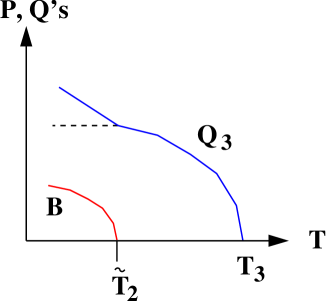
Figure 7: (Color online) Temperature dependence of $Q_{3}$ for $T$ near $T_{3}$ and (lower curve) of $Q_{3}$, $Q_{2}$, and $Q_{5}$ for $T$ near $\tilde{T_{2}}$, as discussed below Eq. (28) and of ${\bf P}$ as described by Eq. (30).

One can similarly analyze the temperature dependence of the strains. From Eq. (24) we see that the strain $\epsilon_{xy}$ (in tetragonal coordinates) is zero for $T>T_{3}$. Just below $T_{3}$ one has

$$\epsilon_{xy}=\alpha[Q_{3}^{-}({\bf q}_{2})^{2}-Q_{3}^{-}({\bf q}_{1})^{2}]/c_{44}\ .$$

Since $Q_{3}\propto(T_{3}-T)^{1/2}$, this indicates that just below $T_{3}$ one has

$$\epsilon_{xy}=\pm(T_{3}-T)\ ,$$

the sign depending on which $Q_{3}({\bf q}_{n})$ has condensed. In addition, the coupling between strains and the orientational OP’s indicate that at the structural transitions there will be a jump in slope of the diagonal strains $\epsilon_{\alpha\alpha}$.

V Coupling to Dielectric and Magnetic Order

In the following two subsections we consider the coupling between the lattice distortions and a) the spontaneous polarization and b) magnetic long range order.

V.1 Dielectric Coupling

The dielectric free energy is

$${\cal F}_{\rm D} = \frac{1}{2}\chi_{E}^{-1}[\vec{P}]^{2}+V_{\rm D}\ ,$$

where $V_{\rm D}$ is the coupling with the distortion modes and which is linear in the spontaneous polarization ${\bf P}$. This coupling will be zero for a structure which has a center of inversion symmetry. $\Gamma_{5}^{-}$ is the only irrep which, by itself, breaks inversion and for it we have

$$V_{\rm D}^{(5)} = -\lambda[Q_{5,1}P_{x}+Q_{5,2}P_{y}]\ .$$

This follows because $Q_{5,1}$ transforms like $x$ and $Q_{5,2}$ transforms like $y$. Using this transformation property, we infer from Eq. (27) a contribution to $V_{\rm D}$ of the form

$$V_{\rm D}^{(2,3)} = -\lambda^{\prime}[Q_{2}({\bf q}_{1})Q_{3}({\bf q}_{1})(P_{x}+P_{y})$$

$$\ +Q_{2}({\bf q}_{2})Q_{3}({\bf q}_{2})(P_{x}-P_{y})]\ .$$

These couplings indicate that

$$P_{x} = \lambda\chi_{E}Q_{5,1}+\lambda^{\prime}\chi_{E}[Q_{2}({\bf q}_{1})Q_{3}({\bf q}_{1})+Q_{2}({\bf q}_{2})Q_{3}({\bf q}_{2})]$$

$$P_{y} = \lambda\chi_{E}Q_{5,2}+\lambda^{\prime}\chi_{E}[Q_{2}({\bf q}_{1})Q_{3}({\bf q}_{1})-Q_{2}({\bf q}_{2})Q_{3}({\bf q}_{2})]\ .$$

We may simplify this by minimizing the free energy of Eqs. (25) and (27) to write

$$Q_{5,1} = \frac{r}{T-T_{5}}\Biggl{(}Q_{2}({\bf q}_{1})Q_{3}({\bf q}_{1})+Q_{2}({\bf q}_{2})Q_{3}({\bf q}_{2})\Biggr{)}$$

$$Q_{5,2} = \frac{r}{T-T_{5}}\Biggl{(}Q_{2}({\bf q}_{1})Q_{3}({\bf q}_{1})-Q_{2}({\bf q}_{2})Q_{3}({\bf q}_{2})\Biggr{)}\ .$$

Thus

$$P_{x} = \tau\Biggl{(}Q_{2}({\bf q}_{1})Q_{3}({\bf q}_{1})+Q_{2}({\bf q}_{2})Q_{3}({\bf q}_{2})\Biggr{)}$$

$$P_{y} = \tau\Biggl{(}Q_{2}({\bf q}_{1})Q_{3}({\bf q}_{1})-Q_{2}({\bf q}_{2})Q_{3}({\bf q}_{2})\Biggr{)}\ ,$$ (30)

where $\tau=\chi_{E}[\lambda^{\prime}+\lambda r/(T-T_{5})]$. As shown in Appendix B, the dielectric constant will have a small amplitude divergence at a temperature $T={\tilde{T}}_{2}$ near $T_{2}$, as is often seen in systems with magnetization induced polarization.[R1, ; R2, ]. Note that there are two mechanisms for a spontaneous polarization proportional respectively to $\lambda^{\prime}$ and $\lambda$. The term in $\lambda$ may be viewed as being the polarization due to displacement of the charged ions in the polar irrep $\Gamma_{5}^{-}$. This displacement is induced by the presence of the other two OP’s $Q_{2}$ and $Q_{3}$. The term in $\lambda^{\prime}$ is due to the modification in the electronic structure proportional to $Q_{2}({\bf q})Q_{3}({\bf q})$ when the displacement due to $\Gamma_{5}^{-}$ is zero. The numerical work of BF indicates that there is a large ($\sim 5\mu{\rm C/cm}^{2}$) spontaneous polarization which arises when $Q_{5}$ is zero and therefore indicates that mechanism b) is dominant.

For $T$ slightly below $\tilde{T_{2}}$, $Q_{3}$ is essentially constant and the other $Q$’s are proportional to $(\tilde{T_{2}}-T)^{1/2}$ within mean field theory, as illustrated in Fig. 7. Equation (30) indicates that ${\bf P}$ is parallel to ${\bf q}$ and is proportional to $Q_{2}Q_{3}$, so that near ${\tilde{T}}_{2}$ one has the mean-field result that $|{\bf P}|\sim(\tilde{T}_{2}-T)^{1/2}$, as shown in Fig. 7. From the work of Mostovoy,[MOST1, ] magnetically induced polarization was not expected to have ${\bf P}\parallel{\bf q}$, although ${\bf P}\parallel{\bf q}$, was found experimentally[RBFE, ] and explained from general symmetry arguments.[RBFE, ; TAK, ] Equation (LABEL:PQEQ) indicates that a polarization will be induced parallel to ${\bf q}$ along one of the four $(1,1,0)$ directions according to the signs of the OP’s as indicated by Eq. (LABEL:PQEQ).

V.2 Magnetism

We now discuss the magnetic structures that can appear in this system. Ca₃Mn₂O₇ becomes antiferromagnetic at $T_{N}=115$K.[LOB, ] For this discussion we will work relative to the parent tetragonal lattice but will introduce the orthorhombic coordinates for the spin vectors so that

$$(S_{X})_{o} = (S_{z})_{t}\ ,\hskip 14.45377pt(S_{Y})_{o}=(S_{x})_{t}+(S_{y})_{t}\ ,\hskip 14.45377pt$$

$$\ (S_{Z})_{o}=(S_{x})_{t}-(S_{y})_{t}\ .$$

In the simplest approximation the antiferromagnetic structure of a single biliayer (consisting of one layer of Mn ions at $z_{t}=x_{o}=\xi$ and another at $z_{t}=x_{o}=-\xi$) is that of two square lattice antiferromagnets stacked directly on top of one another [sites at $(0,0,\xi)$ and $(0,0,-\xi)$], so that all near neighbor interactions proceed via nearly 180^o antiferromagnetic Mn-O-Mn bonds. The first principles calculations of BF and the data from Ref. LOB, indicate that dominantly the spins are perpendicular to the plane. This structure is shown in Fig. 8. Therefore we assume that the dominant order parameter is ${\bf G}({\bf q})$, where we use the Wollan-Koehler[WK, ] symbols to represent the configurations of a single bilayer shown in Fig. 9. In the $G_{z}\equiv G_{X}$ configuration one can have either ${\bf q}={\bf q}_{1}$ or ${\bf q}={\bf q}_{2}$. The difference between $G_{X}({\bf q}_{1})$ and $G_{X}({\bf q}_{2})$ is in the different phase of one bilayer relative to the other. In any case all 5 magnetic nearest neighbors of a central spin are oriented antiparallel to it.

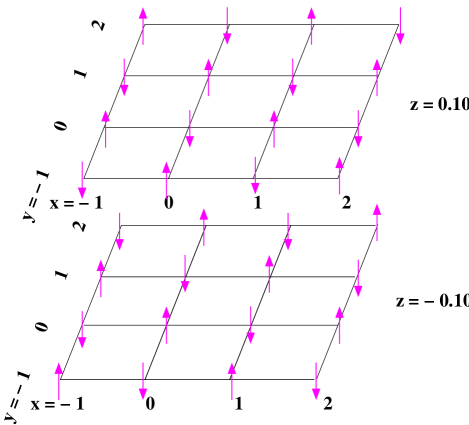
Figure 8: (Color online) A single bilayer of Mn ions when the spins are assumed to lie in the plane. This is a $G_{X}$ configuration. The stacking of adjacent bilayers (not shown) is such that they are displaced transversely by $(1/2,1/2,0)$ relative to one another. The phase of antiferromagnetic order in adjacent bilayers is determined by the wave vector which is either ${\bf q}_{1}$ or ${\bf q}_{2}$. This configuration of pseudovectors is odd under inversion about the origin ($x=y=z=0$).

Figure 9: The A, C, F, and G configurations of spin components for a single bilayer in the Wollan-Koehler[WK, ] scheme.

We will accommodate the following structures based on the parent tetragonal lattice. We have choices for the wave vector, namely ${\bf q}=0$, ${\bf q}={\bf q}_{1}$ and ${\bf q}_{2}$ and $S_{\alpha}(0,0,\xi)=\pm S_{\alpha}(0,0,-\xi)$. So for each component of spin we have six candidate structures. If ${\bf q}=0$ and $S_{\alpha}(0,0,-\xi)=S(0,0,\xi)$, then we have the “F” (ferromagnetic) structure. If ${\bf q}=0$ and $S_{\alpha}(0,0,-\xi)=-S(0,0,\xi)$, then we have the “A” structure shown in Fig. 9. If ${\bf q}={\bf q}_{n}$, then each plane of the bilayer consists of a square lattice antiferromagnet. The two planes of the bilayer can be coupled either so that adjacent spins in the planes are parallel (this is the “C” structure) or so that they are antiparallel (this is the “G” structure), as shown in Fig. 9. The C and G structures each come in two versions depending on whether ${\bf q}={\bf q}_{1}=(1/2,1/2,0)$ or ${\bf q}={\bf q}_{2}=(1/2,-1/2,0)$, as discussed in the caption to Fig. 10. We now introduce orthorhombic coordinates, so that $S_{X}=S_{z}$, $S_{Y}=S_{x}-S_{y}$, and $S_{Z}=S_{x}+S_{y}$. Then we have the symmetries given in Table 3.

Figure 10: Spin states of a bilayer of Mn ions. The plus and minus signs represent the signs of any component of spin. Left: the “A” configuration. Right: the “C” configuration. The circled symbols represent the spins in planes at $z=1/2+\xi$ and $z=1/2-\xi$ for ${\bf q}={\bf q}_{1}$. For ${\bf q}={\bf q}_{2}$ the circled $+$ and circled $-$ signs of the C configuration are interchanged.

Table 3: The symmetry for components $X$, $Y$, and $Z$ of the spin, a pseudovector. Here $S_{X}=S_{z}$, $S_{Y}=S_{x}+S_{y}$, $S_{Z}=S_{x}-S_{y}$, where capitals refer to orthorhombic and lower case to tetragonal.

Structure	${\bf q}$	${\cal I}$			$m_{z}$			$m_{d}$
		$Y$	$Z$	$X$	$Y$	$Z$	$X$	$Y$	$Z$	$X$
F	$0$	$+$	$+$	$+$	$-$	$-$	$+$	$+$	$-$	$-$
A	$0$	$-$	$-$	$-$	$+$	$+$	$-$	$+$	$-$	$-$
G	${\bf q}_{1}$	$-$	$-$	$-$	$+$	$+$	$-$	$+$	$-$	$-$
G	${\bf q}_{2}$	$-$	$-$	$-$	$+$	$+$	$-$	$+$	$-$	$-$
C	${\bf q}_{1}$	$+$	$+$	$+$	$-$	$-$	$+$	$+$	$-$	$-$
C	${\bf q}_{2}$	$+$	$+$	$+$	$-$	$-$	$+$	$+$	$-$	$-$

The magnetic free energy is $F=F_{G}+V$, where $F_{G}$ is the free energy of the G structure:

$$F_{G} = \frac{1}{2}\sum_{\alpha}\Biggl{[}(T-T_{N}+K_{\alpha})\sum_{n}G_{\alpha}({\bf q}_{n})^{2}$$

$$\ -\alpha^{\prime}\sum_{n}G_{\alpha}({\bf q}_{n})^{2}Q_{3}({\bf q}_{n})^{2}\Biggr{]}+{\cal O}[G({\bf q}_{n})^{4}]$$

and

$$V = \frac{1}{2}\sum_{\alpha}\Biggl{[}\mu_{\alpha}F_{\alpha}^{2}+\nu_{\alpha}C_{\alpha}({\bf q}_{1})^{2}+\tau_{\alpha}A_{\alpha}^{2}\Biggr{]}\ .$$ (31)

The quartic term in $F_{G}$ is such as to ensure that the magnetic ordering vector is the same as that of the paramagnetic structure. Now we want to see what other magnetic OP’s are induced by the condensation of the dominant $G$ ordering in the presence of the nontetragonal distortions. The magnetoelastic interaction we invoke has to be quadratic in the magnetic variables in order to be time-reversal invariant. So we consider a cubic potential which contains terms of the form

$$G_{X}({\bf q}_{n})K_{\alpha}Q_{\beta}\ ,$$

where $K$ is $C({\bf q}_{n})$, $F$, or $A$ and $Q$ is $Q_{2}^{+}({\bf q}_{n})$, $Q_{3}^{-}({\bf q}_{n})$, $Z_{5}\equiv Q_{5,1}+Q_{5,2}$, or $Y_{5}\equiv Q_{5,1}-Q_{5,2}$. We start by considering only terms involving ${\bf q}_{1}$. The terms involving ${\bf q}_{2}$ will later be obtained from those involving ${\bf q}_{1}$ by applying the four-fold rotation ${\cal R}_{4}$. The only terms which are consistent with inversion symmetry and wave vector conservation are those of the form

$$G_{X}({\bf q}_{1})A_{\alpha}Q_{2}^{+}({\bf q}_{1})\ ,\ \ \ G_{X}({\bf q}_{1})F_{\alpha}Q_{3}^{-}({\bf q}_{1})\ ,$$

$$\ G_{X}({\bf q}_{1})C_{\alpha}({\bf q}_{1})Z_{5}\ .$$

($Y_{5}=0$ for ${\bf q}={\bf q}_{1}$.) We now use Table 3 to require invariance under $m_{d}$ and $m_{z}$, so that the interaction which has the correct symmetry is

$$aG_{X}({\bf q}_{1})F_{Y}Q_{3}^{-}({\bf q}_{1})+bG_{X}({\bf q}_{1})C_{Z}({\bf q}_{1})Z_{5}\ .$$ (32)

Now we use

$${\cal R}_{4}G_{X}({\bf q}_{n}) = G_{X}({\bf q}_{3-n})\ ,\ \ \ {\cal R}_{4}F_{Y}=-F_{Z}\ ,$$

$${\cal R}_{4}C_{Z}({\bf q}_{1}) = -C_{Y}({\bf q}_{2})\ ,\ \ \ {\cal R}_{4}Q_{3}^{-}({\bf q}_{1})=Q_{3}^{-}({\bf q}_{2})\ ,\$$

$${\cal R}_{4}Z_{5} = Y_{5}\ .$$

Thus, in all, the lowest order magnetoelastic coupling $V_{MQ}$ is

$$V_{MQ} = aG_{X}({\bf q}_{1})F_{Y}Q_{3}^{-}({\bf q}_{1})+bG_{X}({\bf q}_{1})C_{Z}({\bf q}_{1})Z_{5}$$

$$-aG_{X}({\bf q}_{2})F_{Z}Q_{3}^{-}({\bf q}_{2})-bG_{X}({\bf q}_{2})C_{Y}({\bf q}_{2})Y_{5}\ .$$

To see what this means, it is helpful to recall that ${\bf q}_{1}$ (${\bf q}_{2}$) lies along the orthorhombic $Z$ ($Y$) direction. Thus the weak ferromagnetic moment $F$ is perpendicular to ${\bf q}$. Note that the wave vector is already selected as soon as tetragonal symmetry is broken. Say ${\bf q}_{1}$ is selected. Then, in addition, the sign of $Q_{3}^{-}({\bf q}_{1})$ was also selected when tetragonal symmetry was broken. Then, when magnetic long-range order appears, it can have either sign of $G_{X}({\bf q}_{1})$, but the sign of $G_{X}({\bf q}_{1})F_{Z}$ is fixed by the interactions within the system.

Assuming the G configuration to be dominant and using Eq. (31), we thus have two scenarios. If ${\bf q}={\bf q}_{1}$, then we have the magnetic OP’s

$$\ [G_{X}({\bf q}_{1}),F_{Y},C_{Z}({\bf q}_{1})]\ ,\ \ \ \ \ {\rm with}$$

$$\frac{F_{Y}}{G_{X}({\bf q}_{1})}=-\frac{aQ_{3}^{-}({\bf q}_{1})}{\mu_{Z}}\ ,\hskip 14.45377pt\frac{C_{Z}({\bf q}_{1})}{G_{X}({\bf q}_{1})}=-\frac{bZ_{5}}{\nu_{Y}}\ .$$ (34)

If ${\bf q}={\bf q}_{2}$, then we have the magnetic OP’s

$$\ [G_{X}({\bf q}_{2}),C_{Y}({\bf q}_{2},F_{Z})]\ ,\ \ \ \ \ {\rm with}$$

$$\frac{C_{Y}({\bf q}_{2})}{G_{X}({\bf q}_{2})}=\frac{bY_{5}}{\nu_{Z}}\ ,\hskip 14.45377pt\frac{F_{Z}}{G_{X}({\bf q}_{2})}=\frac{aQ_{3}^{-}({\bf q}_{2})}{\mu_{Y}}\ .$$ (35)

In all the above results, since the cubic coupling combines $Z_{5}$ with $Q_{3}^{-}({\bf q}_{1})Q_{2}^{+}({\bf q}_{1})$ and similarly for ${\bf q}={\bf q}_{2}$, we should replace $Z_{5}$ by a linear combination of $Z_{5}$ and $Q_{3}^{-}({\bf q}_{1})Q_{2}^{+}({\bf q}_{1})$ and $Y_{5}$ by a linear combination of $Y_{5}$ and $Q_{3}^{-}({\bf q}_{2})Q_{2}^{+}({\bf q}_{2})$. The result of Eqs. (34) and (35) agrees with the magnetic structure determination of Ref. LOB, and with the symmetry analysis of BF, except that here we emphasize the relation of the magnetic ordering to the preestablished wave vector. These results are summarized by Fig. 11.

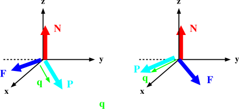
Figure 11: (Color online) The equilibrium orientation of the staggered magnetization (${\bf N}$), the polarization (${\bf P}$), and the weak ferromagnetic moment (${\bf F}$) for ${\bf q}={\bf q}_{1}$ (left panel) and for ${\bf q}={\bf q}_{2}$ (right panel). The axes along which these vectors lie are fixed by symmetry. However, one can find domains in which any (or all) these vectors can be reversed. For instance, ${\bf P}$ is proportional to $Q_{2}Q_{3}$ whereas ${\bf F}$ is proportional to $Q_{3}$.

It is interesting to note the possibility of switching the direction of the polarization (magnetization) by application of a sufficiently strong magnetic (electric) field. For this discussion it is useful ro refer to Fig. 11. Suppose the sample initially has condensed wave vector ${\bf q}_{1}$. (See the left panel of Fig. 11.) Applying a large enough magnetic field in the $Z$ direction (i. e. parallel to ${\bf q}_{1}$) will cause a reorientation of the magnetization of the system so that $F_{Y}=0$ and $F_{Z}\not=0$. Thus $V_{MQ}$ indicates that the system will make a transition from wave vector ${\bf q}_{1}$ to wave vector ${\bf q}_{2}$. Since the direction of the polarization is tied to the direction of the wave vector, this transition will also involve a rotation of the polarization. Likewise, suppose the sample initially has the polarization and the condensed wave vector collinear and parallel to ${\bf q}_{1}$. Equation (34) indicates that the ferromagnetic moment is along $Y$ (which is perpendicular to ${\bf q}_{1}$). Then, if one applies a large enough electric field parallel to ${\bf q}_{2}$, then the polarization will rotate into the direction of ${\bf q}_{2}$ and since the polarization and wave vector are constrained to be collinear, the wave vector will now be along ${\bf q}_{2}$. Then Eq. (LABEL:EQMQ) indicates that the weak ferromagnetic moment will be rotated into the $Z$ direction (which is perpendicular to ${\bf q}_{2}$). However, the applied fields required to accomplish these switchings may be extremely large in view of the structural reorganization involved.

Since $F_{\alpha}$ transforms like a pseudovector, one has symmetry-allowed interactions with $F_{\alpha}$ replaced by $H_{\alpha}$ where ${\bf H}$ is the applied magnetic field. So from Eq. (LABEL:EQMQ) we have a magnetic-field dependent contribution to the free energy of the form

$$V_{\bf H} = c_{1}G_{X}({\bf q}_{1})Q_{3}^{-}({\bf q}_{1})H_{Y}+c_{2}G_{X}({\bf q}_{2})Q_{3}^{-}({\bf q}_{2})H_{Z}\ ,$$ (36)

which indicates that when tetragonal symmetry is broken (so that $Q_{3}$ is nonzero), the magnetic field acts like a field conjugate to the antiferromagnetic OP ${G_{X}}$. Consequently, $\partial G_{X}/\partial H_{\alpha}$ will diverge as the lower transition is approached for $\alpha=Y$ or $\alpha=Z$, according to which wave vector has condensed. This suggests a neutron scattering experiment to measure $G_{X}$ near the lower transition as a function of the magnitude and direction of ${\bf H}$.

VI Domains

Here we discuss in more detail the possible domain structures and give a brief discussion of the dynamics of domain wall motion. We first enumerate the various domains of order parameters which can exist as the temperature is lowered through the various phase transitions. As a preliminary one should note that within a single domain the phase of an OP at wave vector ${\bf q}_{k}$ can not be experimentally determined. However, if more than one such OP is present, then their relative phases can be accessed experimentally. In the discussion that follows we will determine the phase of the OP’s relative to that of $Q_{3}$ which is not determined. As the temperature is lowered through $T_{3}$, four possible domains are created, with the choices of sign of $Q_{3}$ and the two choices for the wave vector, as shown in Fig. 12. The value of the wave vector within a single domain is experimentally accessible via a scattering experiment. Although the phase of $Q_{3}({\bf q})$ can not be established within a single domain, the fact that different such domains do exist can be established by observation of a domain wall separating domains having the same values of the wave vector. Such an experiment to observe a so-called phase domain wall has recently been done in another system.[BODE, ]

Figure 12: Domains in CMO. At $T_{3}$ the value of the wave vector ${\bf q}$ and of $Q_{3}({\bf q})$ are selected. At each succeeding transition a two-state order parameter condenses to further break symmetry. The domains for positive $Q_{3}({\bf q})$ are macroscopically indistinguishable from those for negative $Q_{3}({\bf q})$ because they differ by a unit translation in the $x$-$y$ plane. The signs of the OP’s ${\bf P}$ and the weak ferromagnetic moment ${\bf M}$ depend on the constants $\tau$ of Eq. (30) and $a$ of Eq. (32). For CTO (which is nonmagnetic) the section at and below $T_{N}$ does not apply.

Next, as the temperature is lowered through the lower structural transition at $T={\tilde{T}}_{2}$, the OP $Q_{2}$ is condensed (and, as we have seen, is accompanied by $Q_{5}^{-}$), giving a total of eight domains, four with $Q_{3}>0$ and four with $Q_{3}<0$. These sets of four differ from one another only in the inaccessible phase of the OP $Q_{3}$. However, the four domains having a given sign of $Q_{3}$ can be distinguished from one another, since they correspond to the two choices of wave vector (which is easily experimentally accessible) and the two choices of sign of $Q_{2}$ which leads to distinct orientations of the spontaneous polarization (which is also easily experimentally accessible).

Finally, when the temperature $T_{N}$ is reached, the OP $G_{X}({\bf q})$ which describes the antiferromagnetic order is also accessible because it is coupled to the weak ferromagnetic moment. In that way we can identify the 16 domains up to an uncertainty in the sign of $Q_{3}$. As we indicated above, the uncertainty is, in principle, accessible in that the phase domain wall can be observed. Note that the transformation $(Q_{3},Q_{2},G_{x})\rightarrow(-Q_{3},-Q_{2},-G_{x})$ leaves the observables ${\bf P}$, ${\bf M}$, and ${\bf q}$ invariant.

Figure 13: Displacements of the equatorial oxygens as in Fig. 3. An antiphase domain wall in the phase of a tilted octahedral phase in an $n=1$ RP system. The phases to the left and to the right of the domain wall are indistinguishable since they only differ in the phase of the ordering. In this regard this situation is analogous to domains in an antiferromagnet. If the domain wall were a perfect plane, there would be no distortion energy of the octahedra. However, when the wall has a kink, as shown, then there are two possibilities. First, the tilting a, b, c, d can heal to zero, but this distortion will involve an intraoctahedral distortion of high energy. Secondly, it is possible that a, b, c, d (or analogously e, f, g, h) will alternate in sign, end at an antikink, so that no intraoctahedral energy is involved, but the tilting of the octahedra is not the lowest energy tilting of the established phase and the energy of the kink is proportional to the distance between the kink and the antikink.

The above discussion assumes the existence of domains which, unlike ferromagnetic domains, do not have an obvious energetic reason to exist for $T_{3}>T>{\tilde{T}}_{2}$, where ${\bf P}$ is zero. In particular, the phase domains, if they exist, would appear below the upper ordering temperature $T_{3}$, where $Q_{3}({\bf q})$ condenses, in which one has, for a given wave vector (which can be selected by applying a suitable shear stress), the two possible choices of sign of $Q_{3}({\bf q})$.

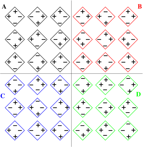
Figure 14: (Color online) Domain walls in CMO for $T_{3}>T>{\tilde{T}}_{2}$. Here one has low energy 90^o walls between phases A and B, B and D, and C and D. Antiphase regions A and D are separated by two such walls. If the distance between regions A and D is not too large, it may be possible to establish the existence of phase domains using the technique of Ref. BODE, .

Upon cooling through $T_{3}$ it seems likely that one would have different nucleation sites from which ordering would develop. As a result, one would have randomly chosen signs of the OP $Q_{3}({\bf q})$ in different regions of the sample. The question then arises, would these domains coarsen and the sample then become a single domain sample? To answer this question we need to study the energetics of domain walls. This involves understanding structural defects, as were studied in Refs. DAVIES, and ARIAS, . For this discussion, I first consider the simpler case of an $n=1$ RP system for which the tilt is around a [100] direction. In Fig. 13 a domain wall is shown separating two phases to the left and right of the wall which differ only in their phase. One sees that if the domain wall is a perfect plane, then there will be no intraoctahedral energy involved in the wall. Indeed, the only energy of the domain wall will be that from the potential that keeps the plane in its location. However, as explained in the caption to Fig. 13, kink formation requires a large energy. Notice the difference between domain walls in this system and those in an Ising antiferromagnet. In an Ising antiferromagnet the domain wall energy is proportional to the length of the wall. Having a kink simply increases the energy by one unit of exchange energy. Here a kink either has the nonlocal string-like energy of a kink-antikink or its has the large energy needed to deform the octahedra. Thus, it seems that domain wall motion may be inhibited and therefore it is possible that phase domains, once created will remain in the sample.

From these examples one concludes that a domain wall tends to form in planes of “minimum contact,” i. e. in planes which intersect the least number of shared oxygen ions. This is why $[100]$ walls are preferred over $[110]$ walls for systems, such as CMO, in which tilting occurs about a $[110]$ direction.[DAVIES, ] Of course, $[001]$ walls (stacking faults) probably have the least energy.

VII CONCLUSIONS

In this paper we have explored the rich structure of structural, magnetic, and dielectric ordering in the Ruddlesden-Popper compound Ca₃Mn₂O₇, using Landau theory to analyze symmetry properties. Our approach is similar to that used by Perez-Mato et al. [PEREZ, ] to study the Aurivillius compounds. Most of the symmetry relations we find are explicitly corroborated by the first principles calculations of Benedek and Fennie. An important aspect of our work is to motivate a large number of experiments which can elucidate the relations between the various order parameters. Specifically, we summarize the conclusions from our work as follows

$\bullet\ 1$ The most important aspect of our work is that we introduce order parameters (OP’s) for all the irreducible representations (irreps) for all the wave vectors of the star which is active in the ordering transitions. The OP’s describe distortions from the parent high symmetry tetragonal lattice which exists at high temperature. This enables us to discuss the induced (nonprimary) OP’s such as the spontaneous polarization, the weak ferromagnetism, and the elastic strains.

$\bullet 2$ In conformity with established results[UTAH, ] (but rejecting multicritical points) we treat the group-subgroup structure obtained by the first principles calculations of Benedek and Fennie.[NATURE, ] We give an OP description of the sequence of structural transitions which is predicted for Ca₃Mn₂O₇ and Ca₃Ti₂O₇, namely I4/mmm $\rightarrow$ Cmcm $\rightarrow$ Cmc2₁ the same as that found for a similar perovskite by Perez-Mato et al..[PEREZ, ]

$\bullet\ 3$ The ordering involves two families of domains, one family for each of the two X wave vectors. At the lower structural transition, a ferroelectric polarization appears parallel to the wave vector. Below that there is an independent magnetic ordering transition to an antiferromagnetic state in which the stacking of the magnetic bilayers depends on the wave vector which was selected when the tetragonal symmetry was broken. A weak ferromagnetic moment develops perpendicular to both the staggered magnetization and the polarization.

$\bullet 4$ We show that by application of an applied magnetic field it might be possible to reorient the ferromagnetic moment through successive 90^o rotations, which would then induce similar rotations of the spontaneous polarization. Likewise, application of an external electric field could reorient the spontaneous polarization which in turn would reorient the wave vector and thereby reorient the weak ferromagnetic moment.

$\bullet 5$ Here we analyzed behavior near the phase transitions using mean field theory. However, non mean-field critical exponents can be accessed experimentally, as has been done for Ni₃V₂O₈.[GLNVO1, ]

$\bullet\ 6$ We have given a detailed enumeration (see Fig. 12) of the domains arising from different realization of the OP’s. We distinguish between domains whose bulk structure is macroscopically identifiable and those (similar to antiferromagnetic domains) that arise from a difference in phase that is not macroscopically accessible. We propose the association of domain walls with planes of “minimum contact” between octahedra. The question of the formation and dynamics of domains (especially those of phase domains) is broached.

Acknowledgments I would like to thank C. J. Fennie for introducing me to this subject and for useful advice. I also thank M. V. Lobanov, H. T. Stokes, B. Campbell, J. M. Perez-Mato, and J. Kikkawa for helpful discussions.

Appendix A Crystal Structure for $Q_{2}^{+}({\bf q}_{1})$ and $Q_{3}^{-}({\bf q}_{1})$

Here we verify that the crystal structure when the OP’s for ireps $X_{2}^{+}$ and $X_{3}^{-}$ at wave vector ${\bf q}_{1}$ are simultaneously nonzero is Cmc2₁. (This result also applies when the OP’s are both at wave vector ${\bf q}_{2}$.) From Table 2 we have the characters listed in Table 4.

Now which operators transform like unity under both irreps? We see that we may choose

$$T_{1}T_{2}\ ,\hskip 10.84006ptT_{1}T_{2}^{-1}\ ,\hskip 10.84006ptT_{1}^{-1}T_{3}\ ,\hskip 10.84006ptm_{z}\ ,\hskip 10.84006ptm_{d}T_{1}\ .$$

These indicate that we new primitive lattice vectors are

$${\bf a}_{1} = (1,1,0)\ ,\hskip 10.84006pt{\bf a}_{2}=(1,\overline{1},0)\ ,\hskip 10.84006pt{\bf a}_{3}=(-1/2,1/2,1/2)\ .$$

Also

$$m_{d} = (x,y,z,)\rightarrow(x,y,\overline{z})\ ,$$

$$m_{d}T_{1} = (x,y,z)\rightarrow(y,x+1,z)$$

Table 4: Characters of generators of the little group for irreps $X_{2}^{+}$ and $X_{3}^{-}$ at wave vector ${\bf q}_{1}$.

${\cal O}=$	${\cal I}$	$m_{d}$	$m_{z}$	$T_{1}$	$T_{2}$	$T_{3}$
$X_{2}^{+}$	1	$-1$	1	$-1$	$-1$	$-1$
$X_{3}^{-}$	$-1$	$-1$	1	$-1$	$-1$	$-1$

To make contact with Ref. ITC, we transform to orthorhombic coordinates:

$$x^{\prime} = z\ ,\hskip 10.84006pty^{\prime}=\frac{x-y}{2}+\frac{1}{4}\ ,\hskip 10.84006ptz^{\prime}=\frac{x+y}{2}\ .$$

In this coordinate system

$${\bf a}_{1}^{\prime} = (0,0,1)\ ,\hskip 10.84006pt{\bf a}_{2}^{\prime}=(0,1,0)\ ,\hskip 10.84006pt{\bf a}_{3}^{\prime}=(1/2,-1/2,0)\ ,$$

and the mirror operations are

$$m_{x}^{\prime} = (x^{\prime},y^{\prime},z^{\prime})\rightarrow(\overline{x}^{\prime},y^{\prime},z^{\prime})$$

$$\ [m_{d}T_{1}]^{\prime} = (x^{\prime},y^{\prime},z^{\prime})\rightarrow(x^{\prime},\overline{y}^{\prime},z^{\prime}+1/2)$$

which coincides with the specification of space group Cmc2₁ in Ref. ITC, . One might object that we have not taken into account the fact that Eq. (27) indicates the presence of irrep $\Gamma_{5}^{-}$. What that means is that this irrep is always allowed in Cmc2₁.

Appendix B CRITICAL BEHAVIOR OF THE DIELECTRIC CONSTANT

The following discussion parallels that given[R2, ] for the dielectric anomaly in Ni₃V₂O₈. We take the free energy (in the ${\bf q}_{1}$ channel) for $T$ near the lower transition [where $Q_{3}({\bf q}_{1})$ is already nonzero] to be

$${\cal F} = \frac{a^{\prime}}{2}(T-T_{2})Q_{2}({\bf q}_{1})^{2}+\frac{a^{\prime\prime}}{2}(T-T_{5})[Q_{5,1}+Q_{5,2}]^{2}$$ (37)

$$\ +w^{\prime}Q_{2}({\bf q}_{1})[Q_{5,1}+Q_{5,2}]-\sqrt{2}\lambda[P_{x}Q_{5,1}+P_{y}Q_{5,2}]$$

$$\ +\frac{1}{2}\chi_{E}^{-1}{\bf P}^{2}-\lambda^{\prime}\langle Q_{3}({\bf q}_{1})\rangle Q_{2}({\bf q}_{1})[P_{x}+P_{y}]$$

$$\ -[P_{x}E_{x}+P_{y}E_{y}]\ .$$

The coupling terms proportional to $\lambda$ and $\lambda^{\prime}$ suggest that the dielectric susceptibility will be singular at the lower transition where $Q_{2}$ and $Q_{5}$ appear. In this appendix we show this explicitly. We write

$$P_{x}Q_{5,1}+P_{y}Q_{5,2} = \frac{1}{2}[P_{x}+P_{y}][Q_{5,1}+Q_{5,2}]$$

$$\ +\frac{1}{2}[P_{x}-P_{y}][Q_{5,1}-Q_{5,2}]$$

and

$$P_{x}E_{x}+P_{y}E_{y} = \frac{1}{2}[P_{x}+P_{y}][E_{x}+E_{y}]$$

$$\ +\frac{1}{2}[P_{x}-P_{y}][E_{x}-E_{y}]\ .$$

Note that in the ${\bf q}_{1}$ channel $Q_{5,1}-Q_{5,2}=0$ and can be dropped. Also, since $E_{x}-E_{y}$ and $P_{x}-P_{y}$ do not couple to a critical variable we drop them too. Now set

$$P \equiv [P_{x}+P_{y}]/\sqrt{2}\ ,\hskip 18.06749ptE\equiv[E_{x}+E_{y}]/\sqrt{2}\ ,$$

$$\ Q_{5}=Q_{5,1}+Q_{5,2}\ .$$

Thus the above free energy is

$${\cal F} = \frac{a^{\prime}}{2}(T-T_{2})Q_{2}^{2}+\frac{a^{\prime\prime}}{2}(T-T_{5})Q_{5}^{2}+w^{\prime}Q_{2}Q_{5}$$

$$+\frac{1}{2}\chi_{E}^{-1}P^{2}-\lambda PQ_{5}-\lambda^{\prime\prime}Q_{2}P-PE\ ,$$

where $\lambda^{\prime\prime}=\lambda^{\prime}\langle Q_{3}({\bf q}_{1})\rangle\sqrt{2}$. Now minimize with respect to $Q_{2}$ and $Q_{5}$ to get

$$\frac{\partial{\cal F}}{\partial Q_{2}} = a^{\prime}(T-T_{2})Q_{2}+w^{\prime}Q_{5}-\lambda^{\prime\prime}P=0\ ,$$

$$\frac{\partial{\cal F}}{\partial Q_{5}} = w^{\prime}Q_{2}+a^{\prime\prime}(T-T_{5})Q_{5}-\lambda P=0\ ,$$

so that

$$Q_{2} = [\lambda^{\prime\prime}a^{\prime\prime}(T-T_{5})-w^{\prime}\lambda]P/D$$

$$Q_{5} = [-\lambda^{\prime\prime}w^{\prime}+a^{\prime}(T-T_{2})\lambda]P/D\ ,$$

where

$$D = a^{\prime}(T-T_{2})a^{\prime\prime}(T-T_{5})-{w^{\prime}}^{2}\ .$$

Then the equation for $P$ is $\partial{\cal F}/\partial P=0$, or

$$-\lambda^{\prime\prime}Q_{2}-\lambda Q_{5}+\chi_{E}^{-1}P=E\ ,$$

so that the dielectric susceptibility is

$${\tilde{\chi}}_{E} \equiv \frac{P}{E}=$$

$$= D\left[a^{\prime}a^{\prime\prime}\chi_{E}^{-1}(T-T_{2})(T-T_{5})-{w^{\prime}}^{2}\chi_{E}^{-1}\right.$$

$$\ \left.-\lambda^{2}a^{\prime}(T-T_{2})-{\lambda^{\prime\prime}}^{2}a^{\prime\prime}(T-T_{5})+2w^{\prime}\lambda\lambda^{\prime\prime}\right]^{-1}\ .$$

Note that ${\tilde{\chi}}_{E}$ has poles at $T={\tilde{T}}_{2}$ (which is close to $T_{2}$) and at ${\tilde{T}}_{5}$ (which is close to $T_{5}$). When the effects of $w^{\prime}$, $\lambda$, and $\lambda^{\prime\prime}$ can be treated perturbatively with respect to $T_{2}$ and $\chi_{E}^{-1}$, we find that

$${\tilde{T}}_{2} = T_{2}+\frac{{w^{\prime}}^{2}}{a^{\prime}a^{\prime\prime}T_{2}}+\frac{{\lambda^{\prime\prime}}^{2}\chi_{E}}{a^{\prime}}\equiv T_{2}+\delta T_{2}$$

a result which is reasonable considering the couplings proportional to $w^{\prime}$ and $\lambda^{\prime}$ in Eq. (B1). For $T$ near ${\tilde{T}}_{2}$ we can therefore write

$${\tilde{\chi}}_{E} = \frac{D\chi_{E}}{a^{\prime}a^{\prime\prime}(T-{\tilde{T}}_{2})(T-{\tilde{T}}_{5})}=\frac{A\chi_{E}}{T-{\tilde{T}}_{2}}\ ,$$

where, in terms of $D(T)$, we have

$$A\approx\frac{D(T={\tilde{T}}_{2})}{a^{\prime}a^{\prime\prime}T_{2}}=\frac{a^{\prime}a^{\prime\prime}T_{2}(\delta T_{2})-{w^{\prime}}^{2}}{a^{\prime}a^{\prime\prime}T_{2}}=\frac{{\lambda^{\prime\prime}}^{2}\chi_{E}}{a^{\prime}}\ ,$$

which is a small amplitude attributable to the existence of the mixing term proportional to $\lambda^{\prime}$ in Eq. (37). But this result does confirm the expected divergence in the dielectric constant at the lower transition where the polarization first appears.

References

- (1) S. N. Ruddlesden and P. Popper, Acta Cryst. 11, 54 (1958).
- (2) D. A. Freedman and T. A. Arias, arXiv:0901.0157.
- (3) K. R. Poepplemeier, M. E Leonowicz, J. C. Scanlon, J. M. Longo, and W. B. Yelon, J. Solid State Chem. 45, 71 (1982).
- (4) M. E Leonowicz, K. R. Poepplemeier, and J. M. Longo, J. Solid State Chem. 71, 59 (1985).
- (5) P. D. Battle, M. A Green, N. S. Laskey, J. E. Millburn, L. Murphy, M. J. Rosseinsky, S. P. Sullivan, and J. F. Vente, Chem. Mater. 9, 552 (1997).
- (6) P. D. Battle, M. A Green, J. Lago, J. E. Millburn, M. J. Rosseinsky, and J. F. Vente, Chem. Mater. 10, 658 (1998).
- (7) I. D. Fawcett, J. E. Sunstrom IV, M. Greenblatt, M. Croft, and K. V. Ramanujachary, Chem. Mater. 10, 3643 (1998).
- (8) D. M. Hatch, H. T. Stokes, K. Aleksandrov, and S. V. Misyul, Phys. Rev. B 39, 9282 (1989).
- (9) K. S. Aleksandrov and J. Bartolomé, Phase Transitions 74, 255 (2001).
- (10) A. B. Harris, arXiv:1012.5127 (2010).
- (11) J. D. Bednorz and K. A. Müller, Z. Phys. B64, 189 (1986).
- (12) Y. Tokura (Ed.), Colossal Magnetoresistance Oxides, Monograph in Condensed Matter Science, Gordon and Breach, London, 2000.
- (13) J. F. Mitchell, D. N. Argyriou, A. Burger, K. E. Grey, R. Osborn, and U. Welp, J. Phys. Chem. B 105, 10732 (2001).
- (14) M. V. Lobanov, M. Greenblatt, El’ad N. Caspi, J. D. Jorgensen, D. V. Sheptyakov, B. H. Toby, C. E. Botez, and P. W. Stephens, J. Phys.: Condens. Matter 16, 5339 (2004).
- (15) L. A. Bendersky, M. Greenblatt, and R. Chen, J. Solid State Chem. 174, 418 (2003).
- (16) A. J. C. Wilson, International Tables for Crystallography (Kluwer Academic, Dordrecht, 1995), Vol. A.
- (17) N. Guiblin, D. Grebille, H. Liligny, and C. Martin, Acta Cryst. C 58, i3 (2001).
- (18) Isotropy Subgroups of the 230 Crystallographic Space Groups, H. T. Stokes and D. M. Hatch, (World Scientific, Singapore, 1988).
- (19) N. A. Benedek and C. J. Fennie, arXiv:1007.1003v2.
- (20) J. M. Perez-Mato, M. Aroyo, A. Garcia, P. Blaha. K. Schwarz, J. Schwiefer, and K. Parlinski, Phys. Rev. B 70, 214111 (2004).
- (21) G. Lawes, private communication.
- (22) M. A. Green and D. A Neumann, Chem. Mater. 12, 90 (2000).
- (23) Y. L. Qin, J. L. García, H. W. Zandbergen, and J. A. Alonso, Phys. Rev. B 63, 144108 (2001).
- (24) W.-H. Jung, J. Mater. Sci. Lett. 19, 2037 (2000).
- (25) S. F. Matar, V. Eyert, A. Villesuzanne, and M.-H. Whangbo, Phys. Rev. B 76, 054403 (2007).
- (26) C. Cardoso, R. P. Borges, T. Gasche, and M. Godinho, J. Phys. Condens. Matter 20, 035202 (2008).
- (27) I. D. Fawcett, E. Kim, M. Greenblatt, M. Croft, and L. A. Bendersky, Phys. Rev. B 62, 6485 (2000).
- (28) Probably BF find that when the spin-orbit interaction is included the spins point along the tetragonal [001] direction as they state. However, there is some confusion, possibly notational, when they state (in the previous sentence) that the polarization is along [010], which would be true if this were in orthorhombic coordinates and were appropriately chosen.
- (29) These irreps are irreps of the full space group for the star of the wave vector. For this irrep is the same as that for the group of the wave vector. For and the matrices for the operators of the group of the wave vector are block diagonal, i. e. they form a reducible representation. However, matrices for operators which are in the full space group but which are not in the group of the wave vector are not diagonal. Therefore this irrep contains information on how the basis functions transform under the operator which is not a member of the group of the wave vector. The first row and column of the matrices refer to and the second ones to .
- (30) See page 2-18 of Ref. UTAH, .
- (31) We put a superscript or on the OP to indicate its parity under inversion when that information needs emphasis.
- (32) See “Hooke’s Law” in Wikipedia (online).
- (33) J. D. Axe, A. H. Moudden, D. Hohlwein, D. E. Cox, K. M. Mohanty, A. R. Moodenbaugh, and Y. Yu, Phys Rev. Lett. 62, 2751 (1989).
- (34) I. Cabrera, M. Kenzelmann, G. Lawes, Y. Chen, W. C. Chen, R. Erwin, T. R. Gentile,J. B. Leão, J. W. Lynn, N. Rogado, R. J. Cava, and C. Broholm, Phys. Rev. Lett. 103, 087201 (2009).
- (35) In BF the number of nonmagnetic domains is quoted as being four. Apparently they did not count the two choices of wave vector.
- (36) The first term in Eq. (23) may not accurately follow a power law for near , but the point we make is that there is an anomaly due to the second term.
- (37) C. R. dela Cruz, B. Lorenz, Y. Y. Sun, Y. Wang, S. Park, S.-W. Cheong, M. M. Gospodinov, and C. W. Chu, Phys. Rev. B 76, 174106 (2007).
- (38) A. B. Harris, Phys. Rev. B 76, 054447 (2007). Erratum, Phys. Rev. B 77, 019901 (2008)
- (39) M. Mostovoy, Phys. Rev. Lett. 96, 067601 (2006).
- (40) M. Kenzelmann, G. Lawes, A. B. Harris, G. Gasparovic, C. Broholm, A. P. Ramirez, G. A. Jorge, M. Jaime, S. Park, Q. Huang, A. Ya. Shapiro, and L. A. Demianets, Phys. Rev. Lett. 98, 267205 (2007)
- (41) T. A. Kaplan and S. D. Mahanti, arXiv:0808.0336v3.
- (42) E. O. Wollan and W. C. Koehler, Phys. Rev. 100, 545 (1955).
- (43) M. Bode, E. Y. Vedmedenko, K. von Bergmann, A. Kubetzka, P. Ferriani, S. Heinze, and R. Wiesendanger, Nat. Mater. 5, 477 (2006).
- (44) B. S. Guiton and P. K. Davies, Nat. Mater. 6, 586 (2007).
- (45) P. Kharel, C. Sudakar, A. Dixit, A. B. Harris, R. Naik, and G. Lawes, Euro. Phys. Lett., 86, 17007 (2009).