Dusty Tori of Luminous Type 1 Quasars at $z\sim 2$

Abstract

We present Spitzer infrared spectra and ultra-violet to mid-infrared spectral energy distributions (SEDs) of 25 luminous type 1 quasars at z $\sim$ 2. In general, the spectra show a bump peaking around 3 ${\rm{\mu}m}$, and the 10 ${\rm{\mu}m}$ silicate emission feature. The 3 ${\rm{\mu}m}$ emission is identified with hot dust emission at its sublimation temperature. We explore two approaches to modeling the SED: (i) using the Clumpy model SED from Nenkova et al. (2008a), and (ii) the Clumpy model SED, and an additional blackbody component to represent the 3 ${\rm{\mu}m}$ emission. In the first case, a parameter search of $\sim 1.25$ million Clumpy models shows: (i) if we ignore the UV-to-near-IR SED, models fit the 2–8 ${\rm{\mu}m}$ region well, but not the 10 ${\rm{\mu}m}$ feature; (ii) if we include the UV-to-near-IR SED in the fit, models do not fit the 2–8 ${\rm{\mu}m}$ region. The observed 10 ${\rm{\mu}m}$ features are broader and shallower than those in the best-fit models in the first approach. In the second case, the shape of the 10 ${\rm{\mu}m}$ feature is better reproduced by the Clumpy models. The additional blackbody contribution in the 2–8 ${\rm{\mu}m}$ range allows Clumpy models dominated by cooler temperatures ($T<800{\rm K}$) to better fit the 8–12${\rm{\mu}m}$ SED. A centrally concentrated distribution of a small number of torus clouds is required in the first case, while in the second case the clouds are more spread out radially. The temperature of the blackbody component is $\sim 1200{\rm\ K}$ as expected for graphite grains.

1. Introduction

In the unified model of active galactic nuclei (AGN) (Antonucci 1993; Urry & Padovani 1995), the dust torus is a region immediately outside the accretion disk where dusty clouds are no longer sublimated by the radiation from the central engine. The dust torus reprocesses the incident ultra-violet/optical radiation from the accretion disk and this energy emerges in the near- and mid-infrared bands. Richards et al. (2006) presented panchromatic spectral energy distributions (SEDs) for 259 type 1 quasars selected from the Sloan Digital Sky Survey (SDSS, York et al. 2000). These quasar SEDs constructed from broad-band photometry are remarkably similar over a large range in both luminosity and redshift. However, Richards et al. (2006) noted small differences in the 1.3–8 ${\rm{\mu}m}$ range between optically luminous and optically dim quasars. Gallagher et al. (2007) investigated this further, and found that the 1–8 ${\rm{\mu}m}$ spectral index ($\alpha_{\nu}$) is strongly anti-correlated with infrared luminosity in type 1 quasars. More luminous quasars have bluer 1–8 ${\rm{\mu}m}$ slopes. Further, they noted a tight linear correlation between the ultra-violet (UV) continuum luminosity and the infrared luminosity for these quasars. This suggested that the observed near-IR emission at $3\ {\rm{\mu}m}$ in the SED of many type 1 objects is driven by the dust reprocessing of the intrinsic optical/ultra-violet continuum from the accretion disk, as had been noted previously (Rees et al. 1969; Neugebauer et al. 1979; Edelson & Malkan 1986; Barvainis 1987; Sanders et al. 1989). As a recent example, the near-IR emission is clearly visible in the spectrum of Mrk 1239 (Rodríguez-Ardila & Mazzalay 2006).

Theoretical work on the response of accretion disks to radiation and hydromagnetic pressure suggests that outflow of matter is associated with all accretion disks in the form of a wind coming off the surface of the disk (Konigl & Kartje 1994; Murray & Chiang 1995; Proga et al. 2000). The dusty torus itself may be the outermost part of this accretion disk wind close to the equator of the system (Konigl & Kartje 1994; Elitzur & Shlosman 2006). Disk-winds have a natural dependence on luminosity through radiation pressure, and this begs the question: “is the structure of the dusty torus related to the physics of the accretion disk?”. The need for proper radiation transfer treatment of clumps in dusty tori was recognized in the pioneering early studies (Krolik & Begelman 1988; Pier & Krolik 1992; Rowan-Robinson 1995), and was fully developed by Nenkova et al. (2002). More recently, Nenkova et al. (2008a) presented their model in detail (denoted by Clumpy hereafter).

Significant effort has been invested in understanding the torus dust distributions with various groups favoring both clumpy and smooth dust density distributions (Nenkova et al. 2002; Dullemond & van Bemmel 2005; Schartmann et al. 2005; Fritz et al. 2006; Hönig et al. 2006; Schartmann et al. 2008; Nenkova et al. 2008a). The primary difference between clumpy and smooth models is that of the dust temperature distributions (see Fig. 3 of Schartmann et al. 2008). While in smooth density models, the temperature steadily declines with radius from the inner wall, clumpy models can show a range of temperatures at different distances from the central source. This effect occurs primarily due to the shadowing effect from the finite size of clouds. The inner faces of clouds are directly exposed to radiation from the central source, and are hence hotter, while their outer faces are much cooler. And because of clumpiness, clouds farther out in radius can still have their inner faces exposed directly to radiation from the central source.

The effective optical depth in a clumpy torus is a function of the number density of clouds in the central regions of the torus. This important model construction has resulted in better fits to both low-resolution Spitzer spectra (Mor et al. 2009; Nikutta et al. 2009), and high-resolution interferometric observations of dust tori in NGC 1068 (Jaffe et al. 2004) and Circinus (Tristram et al. 2007).

Clumpy models appear to be the most promising set of models with a wide range of applications to both active galactic nuclei (AGN) (e.g., Mason et al. 2006) and merger-driven ultra-luminous infrared galaxies (ULIRG) (Levenson et al. 2007). Other notable models that employ clumps arranged in a disk-like geometry include Schartmann et al. (2008) and Hönig et al. (2006). For example, Polletta et al. (2008) employed clumpy torus models from Hönig et al. (2006) to fit their optically obscured but infrared-bright sources at high-redshift.

Clumpy models show changes in their near-IR continua based on the average number of clouds ($N_{0}$) encountered along a radial equatorial ray (see Fig. 6 in Nenkova et al. 2008b). Using Spitzer mid-IR spectroscopy of high redshift quasars it is then possible to constrain the parameters of their dusty tori. While Spitzer archives are rich in observations of low-redshift Seyfert galaxies, they are deficient in high-redshift observations of radio-quiet quasars at the peak of the quasar activity in the Universe. In this paper, we present such observations as obtained with the Infrared Spectrograph (IRS) on board Spitzer. Our goals include: (1) presenting high-quality mid-IR quasar spectra covering rest-frame 2–12${\rm{\mu}m}$ for comparison to the low-redshift templates already available (e.g., Hao et al. 2005; Weedman et al. 2005; Buchanan et al. 2006; Glikman et al. 2006; Shi et al. 2006; Schweitzer et al. 2006); (2) testing the validity of Clumpy torus models by fitting the observed spectra with model SEDs. Using good-quality IRS spectra we hope to model the 10 ${\rm{\mu}m}$ region properly and constrain Clumpy torus parameters for these luminous quasars.

The properties of the sample and reduction process of the IRS spectra are presented in Section 2. The IRS spectra and SEDs of the sample are discussed in Section 3. Clumpy torus models are summarized in Section 4, and Section 5 presents results of model fits to ultra-violet to mid-IR SEDs. Results are summarized in Section 7. In all calculations, we assume a standard cosmology with $H_{0}=71{\rm\ km\ s^{-1}\ Mpc^{-1}}$, $\Omega_{\rm{M}}=0.27$, and $\Omega_{\rm{Vac}}=0.730$.

2. Data

2.1. The Sample

Our primary sample includes those quasars from Richards et al. (2006) that are 1) in the 1.6–2.2 redshift range, 2) not BAL quasars, and 3) require IRS exposure times less than 2 hours to achieve S/N $\sim 15$ in each of the four IRS low resolution bandpasses. There are 25 such objects in the Richards et al. (2006) sample. Four of these have already been targeted by IRS (Program 3046, PI: I. Perez-Fournon). Most objects from this sample also have Spitzer InfraRed Array Camera (IRAC, Fazio et al. 2004) observations from the Spitzer Wide-area InfraRed Extragalactic (SWIRE) survey (Lonsdale et al. 2003).

The redshift range 1.6–2.2 was chosen to provide rich diagnostics in both the optical and ultra-violet via SDSS spectroscopy and photometry, and in the mid-IR range via Spitzer observations. At these redshifts, the SDSS spectroscopy samples the crucial 1000–3500Å range giving a direct measurement of the strength and shape of the ultra-violet (UV) continuum. The 1.6–2.2 redshift range allows the rest-frame 2–14 ${\rm{\mu}m}$ range to be redshifted into the IRS low-resolution bandpass of 5.2 to 38 ${\rm{\mu}m}$. The IRAC bandpasses (at 3.6, 4.5, 5.8, and 8.0${\rm{\mu}m}$) provide coverage of the rest-frame 1–3 ${\rm{\mu}m}$, thus sampling rest frame 1–14${\rm{\mu}m}$. The model torus SED changes significantly in this region depending on the average number of clouds along the line of sight, their average temperatures and radial distributions (see Fig. 6 in Nenkova et al. 2008b).

The objects chosen are listed in Table 1, along with a summary of the low-resolution spectroscopic observations. The Spitzer IRS low-resolution data comes mainly from programs 50087 (PI: G.T. Richards, 16 objects), 50328 (PI: S.C. Gallagher, 5 objects) and 4 archival datasets from program 3046 (PI: I. Perez-Fournon) as mention above. Out of the 16 objects for which observations were requested in program 50087, we were able to obtain observations of 15 objects and 1 observation (SDSSJ163021) failed to a peak-up lock on a nearby bright star-forming galaxy instead of the quasar. Only this source does not have an IRS spectrum, but we use its SED for analysis. Model fits for this source are unreliable due to lack of IRS spectrum. All 5 objects from program 50328 were observed. Table 2 provides the photometric measurements as obtained from the SDSS DR7 catalogue along with absolute $i$-band magnitude and $\Delta(g-i)$ values (see figure 5 of Richards et al. 2003). The redshifts in Table 2 are taken from updated SDSS redshift catalog provided by Hewett & Wild (2010). Table 3 provides the 2MASS, IRAC and MIPS measurements from the 2MASS and SWIRE databases. Table 4 provides continuum measurements from the reduced IRS spectra at 3, 5, 8 and 10 ${\rm{\mu}m}$ in the rest-frame.

2.2. Data Reduction

We obtained the basic calibrated data (BCD) products processed with the standard Spitzer IRS pipeline (version S18.7.0) from the Spitzer Science Center (SSC) archive. We cleaned the BCD images using the IRSCLEAN software package to fix rogue pixels using SSC supplied masks, and a weak thresholding of the pixel histogram. We co-added the multiple data collection event (DCE) image files into one image for each module, spectral order and the “nod” position (e.g., SL, 1st order, 1st nod-position) using the fair-coadd option in SMART. We differenced the co-added images from the opposite “nod” positions to remove the sky background. The spectra were extracted using the optimal extraction option within the SMART package. All the image combining and spectrum extraction operations were carried out using SMART (Higdon et al. 2004). We also checked our extractions using the SPICE program. We obtained average S/N of $\sim$6–10 for 4 archival spectra from program 3046, $\sim$ 10–13 for spectra from program 50087, and $\sim$ 25–35 for the spectra from proposal 50328. These S/N estimates were commensurate with the pre-determined configuration of each observation. Figure 1 displays the observed spectra plotted along with SEDs.

3. Spectra and SEDs

In general, the spectra show two features peaking at $\sim 3$ and $\sim 10\ {\rm{\mu}m}$ (see Figure 1, features are marked by vertical dashed lines) in $\nu L_{\nu}$ units. The infrared spectral index ($\alpha_{\nu}$) from 3–8 ${\rm{\mu}m}$ ranges from -0.49 to -1.82, with a median of -0.86. The 10 ${\rm{\mu}m}$ emission feature is the well-known 10 ${\rm{\mu}m}$ silicate emission feature due to the Si-O stretching mode of the silicate molecule. This emission feature was well-known in stellar spectra for a long time (e.g.,  Little-Marenin & Little 1988), but has only recently been detected in quasar spectra (Siebenmorgen et al. 2005; Hao et al. 2005; Sturm et al. 2005) due to the sensitive spectroscopy and broad wavelength coverage possible with Spitzer.

The weakness of the 10 ${\rm{\mu}m}$ emission feature in IR spectra of local type 1 AGN had motivated suggestions of presence of different chemical compositions and/or size distributions of dust grains (Laor & Draine 1993; Maiolino et al. 2001). Instead Clumpy models of (Nenkova et al. 2002) make use of the clumpy nature of the dusty medium to improve model fits to the 10 ${\rm{\mu}m}$ region. However, as we will see ahead, different sublimation temperatures and radii for graphite and silicate grains remain an important issue to be resolved in torus models.

The emission peaking between 2 and 4 ${\rm{\mu}m}$ can be attributed to the blackbody emission from dust close to its sublimation temperature (Rees et al. 1969; Davidson & Netzer 1979; Barvainis 1987), which is typically expected to be $T\gtrsim 1500{\rm\ K}$ for graphite dust. This hot dust emission has long been expected based on broad-band IR data (Sanders et al. 1989). Measurement of the strength of this feature relative to longer wavelength mid-IR emission is important because it can give constraints on the inclination of the torus assuming a disk-like configuration (Pier & Krolik 1993; Murayama et al. 2000). Recent advances in near-IR ground-based spectroscopy has lead to observations of the near-IR bump in Mrk 1239 (Rodríguez-Ardila & Mazzalay 2006) and NGC 4151 (Riffel et al. 2009).

Figure 1 shows the SEDs constructed using the photometric data points from Tables 2, 3, and 4. Also over-plotted for each object is the IRS spectrum along with the mean quasar SED template from Richards et al. (2006) scaled to the SDSS $i$-band luminosity for each object. While the mean SED captures the overall trend quite well, individual spectra reveal significant differences from the mean SED. Objects with similar UV luminosities can have different relative IR power ($\sim$ 0.3 dex). Obscured sources (for e.g., SDSSJ142730, program 50087) are significantly more IR luminous than sources with similar observed UV luminosities (for e.g., SDSSJ172522, program 50087) that are probably not as strongly obscured based on their optical SDSS spectra. This trend is reflected in the mean SEDs constructed by Richards et al. (2006).

4. CLUMPY Torus Models

We use the Clumpy torus models from Nenkova et al. (2008a) to fit the complete SEDs. The models are constructed by assuming an intrinsic AGN SED that heats the dust clouds (see Figure 4 of Nenkova et al. 2008a). We do not considered the effects of a different intrinsic AGN SED. This effect was partially studied by Nenkova et al. (2008a) (see their Fig. 12), and it is expected that the SED longward of 1 micron should not change significantly. Clumpy models contain a standard Galactic mix of silicates (53%) and graphite (47%) dust grains. We have not explored changes in composition, and size distribution of dust grains (see e.g.,  Laor & Draine 1993), and contributions from species other than silicates (e.g.,  Markwick-Kemper et al. 2007). These areas should be addressed by future work on torus models.

The Clumpy torus model is realized as a collection of individual molecular clumps/clouds arranged in a toroidal structure around the central accretion disk. In reality, this region is likely to be a continuous extension of the outer accretion disk (Elitzur & Shlosman 2006). The primary parameters of the Clumpy torus model are described below.

1. $N_{0}$: It is the average number of clouds along a radial equatorial ray in a given model. It represents the normalization of a Gaussian distribution of clouds around the equatorial plane. The total number of clouds intersecting a given equatorial ray is different for different lines of sight. The intrinsic AGN continuum can escape along many different lines of sight, and the observed mid-infrared 10 ${\rm{\mu}m}$ silicate features can be seen in emission even for lines of sight close to the equator. The total effective optical depth to the continuum source is thus a function of the number of clouds along the line of sight and optical depth of each cloud.

2. $\tau_{V}$: Each of the clouds/clumps are assumed to have the same optical depth $\tau_{V}$ in the V-band. Assuming standard Milky Way dust extinction with $R_{V}=3.1$, $A_{V}/\tau_{9.7{\rm{\mu}m}}=18.0\pm 1.0$ (Roche & Aitken 1984; Whittet 2003), and $A_{V}=1.086\,\tau_{V}$; only when $\tau_{9.7{\rm{\mu}m}}\geq 1$ or $\tau_{V}\gtrsim 16.5$, we will notice the effects of self-absorption on the 10 ${\rm{\mu}m}$ feature.

3. $Y$: The radial extent of the torus $Y$, which is the ratio of the outer ($R_{o}$) to the inner radius ($R_{d}$) of the torus. The inner radius depends on the onset of dust sublimation due to the incident UV radiation from the accretion disk (Barvainis 1987). See also Eq. 1 in Nenkova et al. (2008b). The radial extent $Y$ of the torus decides the infrared turn-over at long wavelengths ($\lambda\gtrsim 30\ {\rm{\mu}m}$).

4. $q$: The clouds are distributed along the radius with a power-law distribution ($r^{-q}$) parametrized with the exponent “$q$”. For $q>1$, the clumps are concentrated closer to $R_{d}$. When the clumps are packed closer to $R_{d}$, the resultant infrared SED is dominated by the emission from dust close to its sublimation temperature, and there is little long-wavelength mid-IR emission. The corresponding width of the SED (Pier & Krolik 1993) in this case is also small.

5. $\sigma$: The torus angular width $\sigma$, is the width of the Gaussian distribution of clumps around the equatorial plane. Thick tori (large $\sigma$) generate redder 3–8 ${\rm{\mu}m}$ continua (in $\lambda F_{\lambda}$ units).

6. $i$: The models produce the infrared SED longward of $\sim 1~{}{\rm{\mu}m}$ for each inclination $i$ from $0^{\circ}$ (face-on) to $90^{\circ}$ (edge-on) in steps of $10^{\circ}$.

The torus models are constructed using the radiative transfer code, Clumpy (Nenkova et al. 2002). The tabulated SEDs for different parameters are accessible from the Clumpy project website.

Clumpy dust density distributions differ from smooth distributions in one important aspect: in smooth dust distributions the temperature is uniquely determined by the distance from the source of radiation. While this is also roughly true for clumpy distributions, the presence of lines of sight with different dust columns allows both hot and cold temperature regions to co-exist at similar radial distances. This leads to a greater dependence of the output SED on $N_{0}$, $\tau_{V}$ and $q$. The primary motivating factor for considering clumpy models for the torus is interferometric observations of local AGN (Jaffe et al. 2004) which constrain the tori to be physically small ($R_{o}\lesssim\rm{a\ few}{\rm\ pc}$).

5. Model Fits

To fit our data with the Clumpy torus models, we adopt the procedure developed by Nikutta et al. (2009). We analyze the distributions of best fitting Clumpy torus parameters for each quasar in our sample. We consider the following grid of parameters,

• $q$ = 0.0–3.0, in steps of 0.5

• $N_{0}$ = 1–15, in steps of 1

• $\tau_{V}$ = 5, 10, 20, 30, 40, 60, 80, 100, 150

• $Y$ = 5, 10, 20, 30, 40, 50, 60, 70, 80, 90, 100

• $\sigma$ = 15–70, in steps of 5

• $i$ = 0–90, in steps of 10

in all, $\sim 1.25$ million possible combinations of model parameters. Very large values of $Y$ and $\tau_{V}$, present in the original model grid in Nikutta et al. (2009), are excluded here as the objects under study are type 1 quasars; with, in most cases silicate 10${\rm{\mu}m}$ feature in emission.

Each model is scaled and fitted such that the overall fitting error $E$ is minimized. We adopt Eq. 1 from Nikutta et al. (2009) shown below.

$$E=\frac{1}{N}\sqrt{\sum^{N}_{i=1}\left(\frac{F_{AGN}\cdot f_{i}^{m}-f_{i}^{\rm{obs}}}{\sigma_{i}}\right)}$$ (1)

Here, $f_{i}^{\rm{obs}}=\lambda_{i}F_{i}$, are the observed SED data points that are interpolated at model grid points denoted by $\lambda_{i}$ (see ahead for why we take this approach); $f_{i}^{m}$ are the corresponding model SED points; $\sigma_{i}$ are the 1-$\sigma$ errors on $\lambda_{i}F_{i}$. The scaling of the model, $F_{AGN}$, provides a measure of the infrared luminosity of the Clumpy torus, which can be converted into an estimate of the bolometric luminosity of the system.

For each parameter, we construct a discrete distribution of values by selecting a sample of well-fit models. For each model, the fitting error $E$ is computed from Eq 1. The model with minimum value of fitting error, $E_{\rm Min}$, is considered to be the best-fit model. Further, a relative error, $E_{r}=100\times\left|E-E_{\rm Min}\right|/E_{\rm Min}$, for each model is constructed. Models that differ by 10% from the minimum value $E_{\rm Min}$ are considered to represent the distribution of parameter values that best represents the data for a given quasar. For each parameter, we consider the mode of the distribution of parameter values as the most probable value of the parameter for a given quasar. Note that the best-fitting value may not be the most probable one. The 90% confidence intervals for a parameter are also computed.

The model SEDs are scaled, and fitted to the data SEDs constructed from the photometric data, and the IRS spectrum. We attempt the fitting procedure for all 1.25 million model SEDs, and record their respective relative error $E_{r}$. Parameter distributions are then constructed where the acceptance criteria to form the samples are $E_{r}\sim$ 10%, 20% and 30%. We find that the distributions gradually become flatter or uniform as the relative error criterion is relaxed. Thus, a narrower distribution suggests a better constrained parameter value.

To measure how well a parameter is constrained we use the discrete Kullback-Leibler divergence. The KL divergence measures the similarity of two histograms (or discrete distributions) of identical sampling $k$. The KL divergence is written as,

$$D_{KL}=\sum_{k}Po_{k}*\log_{2}(Po_{k}/Pr_{k})/\log_{2}(N)$$

with $N$ the number of sampled bins, $Pr$ the prior distribution of parameter values (uniform in this analysis), and $Po$ the posterior distribution of parameter values (histogram of “accepted” parameter values). The normalization $\log_{2}(N)$ ensures that $D_{KL}=1.0$ when all accepted models happen to have a parameter value within a single bin. A $D_{KL}$ value close to 1 indicates a better constrained parameter.

Figure 2 shows the parameter distributions corresponding to three sources from our sample for brevity. For each parameter there are three figures from left to right corresponding to the three sources: SDSSJ100401.27+423123.0, SDSSJ160950.72+532909.5, and SDSSJ142730.19+324106.4. SDSS100401 shows strong near-IR emission, and has high UV luminosity (Figure 1). SDSSJ160950 is weak in the UV and also has weak 3 and 10 ${\rm{\mu}m}$ features; SDSS142730 has a deep 10 ${\rm{\mu}m}$ absorption feature. This source shows a power-law optical/UV continuum in its SDSS spectrum, but its emission lines are absorbed (and may be a BALQSO), which is consistent with its mid-IR nature. For each source, we show the distribution of Clumpy parameter values that forms by accepting models that fall within 10% of the best-fit model.

It should be noted that we are fitting the entire SED from UV to MIR, and the IRS range is more densely sampled than the photometry. To avoid problems due to uneven spectral sampling, the data SED was resampled to the wavelength grid of the models. This is not a significant issue since we are interested in fits to the broad-band features of the SED such as the optical AGN power-law, the near-IR bump and the 10 ${\rm{\mu}m}$ feature. The Clumpy model SED is better sampled near 9.7 ${\rm{\mu}m}$ than elsewhere, thus, this improves the fit to the 10 ${\rm{\mu}m}$ region without biasing the fit to be weighted more by the 2–8 ${\rm{\mu}m}$ continuum. Another important point to be noted is that the selection of the model (AGN+TORUS) SED is also constrained by the optical/UV portion of the data SED. While we do not investigate changes in the intrinsic AGN SED, by including fits to the optical SDSS photometry, we are preferentially selecting model SEDs that satisfy consistent flux density scaling in both UV and mid-IR regime at the same time.

5.1. Model fits using the Clumpy SED

Initially, we used only the Clumpy model SED to fit the data SED. The best-fit values of the parameters for each model are given in Table 5. Example model fits are shown in the left-hand panels of Figure 3. The best-fitting models of the entire sample have $N_{0}\sim 1$, $\tau_{V}\sim$ 20–100, $q\gtrsim 2$, $\sigma\sim 15$, and $i\sim$ 60–80 (see Table 5 and dark bars in Figure 2). The radial extent $Y$ of the torus is unconstrained with parameter distributions nearly flat over the sampling grid.

We find that models with $N_{0}\sim 1$, $q\sim 3$, $\tau_{V}\lesssim 10$, $Y\sim 5$, and $\sigma\sim 15$ show peaked 10 ${\rm{\mu}m}$ silicate emission features for all values of the inclination of the line of sight. For $\tau_{V}\lesssim 15$, all wavelengths longer than $\sim 1.5\,{\rm{\mu}m}$ have $\tau<1$, and the dust emission is optically thin (Nenkova et al. 2008b). In this case, the SED simply follows the shape of the dust absorption co-efficients, which decreases rapidly at longer wavelengths in the mid-IR. The observed spectra should then have blue 3–8 ${\rm{\mu}m}$ continua, which is indeed the case for luminous objects like SDSS100401 and SDSSJ151307 (both from program 50328), as can be seen in Figure 1, bottom row of panels.

Further, $q$ is well-constrained in the case of single-component models to a high value of 2–3 in the case of most objects. This suggests a steep radial distribution of clumps, with most clumps concentrated close to $R_{d}$. Nenkova et al. (2008a) show that whenever $q\gtrsim 2$, $Y$ is fundamentally unconstrained. As most clumps are closer to $R_{d}$ in this case, the absolute size of the torus does not matter; the output SEDs from tori of all sizes look the same. On the other hand, for sources with $q\sim 0$, the clump distribution is flatter/spatially extended, and $Y$ can be constrained much better for such sources as cooler temperatures contribute at longer wavelengths.

Increasing $N_{0}$, $\tau_{V}$, and/or $Y$ causes the SED to become redder in the 2–8 ${\rm{\mu}m}$ wavelength range, and the overall flux density peak shifts to longer mid-infrared wavelengths (due to the Wien displacement law). The increasing $N_{0}$ and $\tau_{V}$ essentially increases the obscuration due to the torus, and leads to increased contribution from the cooler parts of the clouds. This effect can be seen by comparing best-fit values of $N_{0}$ for SDSS142730 (Table 5) with the rest of the sample. Larger $N_{0}$ at smaller $\tau_{V}$ and small $Y$ apparently still produce deep absorption features. Larger $Y$ has similar effect if $q\lesssim 1$, as clouds are more spread out radially, and hence cooler. Thus, detecting a blue SED in the 2–8 ${\rm{\mu}m}$ range suggests small $N_{0}$, $\tau_{V}$, and $Y$, along with a radially steep distribution ($q\gtrsim 1$) of clouds. This conclusion however comes with a caveat: while it is clear that the near-IR emission is generated by the dust close to its sublimation point, the strong silicate emission features predicted by the Clumpy models with these parameter configurations are not observed.

The near-IR emission is fitted well by Clumpy models with $N_{0}\sim 1$, $\tau_{V}\sim 5$ and $q>1$, the 10 ${\rm{\mu}m}$ feature profiles are not well-fit by the same models. The model 10 ${\rm{\mu}m}$ profiles are more peaked than observed profiles, which are broad and shallow. We note that this uncertainty about the origin of the near-IR emission in torus models was also encountered previously in the study by Pier & Krolik (1993), where they also had to employ an additive blackbody component to represent the near-IR contribution separate from their mid-IR torus component. Even in smooth density models, where dust temperatures are functions of radial distance from the source, use of a common sublimation temperature for graphite and silicate dust leads to this effect. Using different sublimation radii for different grain populations is computationally expensive, which could explain some of these discrepancies.

Fitting UV/optical continuum and mid-IR together highlights the need for an additional blackbody component (see left panels of Figure 3). Polletta et al. (2008, see their Figure 1) also came to similar conclusions in their effort to fit high-z extremely obscured sources with clumpy torus models from Hönig et al. (2006). This appears to be a common problem to all clumpy models constructed so far.

5.2. Additive Near-IR Blackbody Emission

To improve fits to the 10 ${\rm{\mu}m}$ features, we considered a linear combination of a blackbody and a Clumpy SED (hereafter Clumpy+Blackbody model) as explored also by Mor et al. (2009) for PG quasars. The best-fit values of the parameters for this model are given in Table 6. The model fits are shown in the middle panels of Figure 3.

The additive blackbody component represents emission from the very hot dust at the inner edge of the torus. Clumpy models use standard Galactic dust composition consisting of both silicates (53%) and graphite (47%). The blackbody emission around $3\ {\rm{\mu}m}$ is expected to be a result of emission from graphite grains. As we saw in the last section, this emission can be matched using Clumpy models with $N_{0}=1$, $q>1$, $\tau_{V}\sim$ 5–10. The problem is not matching the near-IR blackbody emission, but matching the 10 micron emission using the same model parameters. The silicate emission in these models is stronger than observed in the spectra. This is likely to be an artifact of constructing a single dust grain type that is a linear combination of individual grain emission efficiencies. This approach is taken in DUSTY (Ivezić et al. 1999), the underlying radiation transfer code for Clumpy . Requiring a fit to only the 10 micron region selects models with weak emission at 3 microns. Additional blackbody contribution above that obtained from the Clumpy models possibly indicates the presence of an extended graphite zone, where silicates are depleted, something that is not accounted for by Clumpy models assuming a single composite grain type at all radii. This extended graphite zone may have a smooth density profile.

The Clumpy+Blackbody models provide better fits to the 10 ${\rm{\mu}m}$ feature (see panels on the right in Figure 3). A much larger range of model parameters becomes accessible (see Table 7) due to the addition of the hot blackbody component. However, this process also weakens any constraints that could be placed on $N_{0}$, $\tau_{V}$ and $q$ as a larger number of models are now accepted by the relative error criterion. Thus, an additive blackbody is but a temporary stop-gap, until the models are expanded. Since the additive blackbody is ad-hoc, the resulting total model SED is phenomenological in nature.

Overall, the Clumpy+Blackbody models prefer more extended tori ($q\sim 1$, $Y\sim$ 50–100) with a somewhat larger number of clouds ($N_{0}\sim$ 5–15) of large optical depths ($\tau_{V}\sim$ 40–150) and high inclinations $i\sim 80$^o. Our sources are selected to be type 1 objects, and we expect the inclination of our line of sight to be smaller than $\sim 60^{\circ}$. In the case of Clumpy+Blackbody model, $q$ appears to be constrained only for source SDSSJ142730, which has a deep 10 ${\rm{\mu}m}$ absorption feature. The torus angular width $\sigma$ is relatively better constrained in the Clumpy+Blackbody models than in the single-component model (See Table 7).

The median ratio of integrated flux ($\lambda F_{\lambda}$ longward of 1 micron) between the blackbody and the Clumpy model is $0.19\pm 0.11$ for our objects. In most luminous objects, this ratio is about $0.15$, which suggests that the very hot dust emits a small portion of the $L_{\rm IR}$ (see also Pier & Krolik 1993), and the bulk of the emission occurs in the “warm” 8–25 ${\rm{\mu}m}$ part of the torus, and this part also likely contains most of the dust mass because the dust emissivity decreases at longer wavelengths.

It is interesting to note that in the case of the Clumpy+Blackbody model the $D_{KL}$ values are not close to 1 for all parameters, which suggests that multi-component fits weaken the constraints the near-IR data put on torus model parameters. Adding a blackbody component makes constraining Clumpy torus parameters difficult without additional far-IR data. Observations using the Herschel space observatory will likely provide a measure of the contribution of the torus against that contributed by circum-nuclear star formation (Netzer et al. 2007, see their Figure 6), and allow better constraints to be put on the torus models in the long-wavelength regime.

6. Observed Silicate Features

The 10 ${\rm{\mu}m}$ silicate emission feature gets broader and weaker with increasing $\tau_{V}$, $N_{0}$, $\sigma$, and $Y$. None of our objects show peaked 10 ${\rm{\mu}m}$ silicate emission profiles in the spectra, indicating that hot dust generating the near-IR emission is depleted in silicate dust, and that the 10${\rm{\mu}m}$ region receives contribution from multiple “colder than sublimation temperature” sources which likely make the feature broader and weaker. Right-hand panels in Figure 3 show the fits of silicate features in the presence of an extra blackbody component.

In most objects, the feature either peaks around 9.7 ${\rm{\mu}m}$ (SDSS100401) or is mostly flat (SDSS160950). In some cases, there is a well-defined plateau from 9.7 to 11.4 ${\rm{\mu}m}$ (SDSS151307, last right-most panel in Figure 3). We find that with the Clumpy+Blackbody fits, the models mostly reproduce the observed shapes within the errors of the observations, with the exception of emission around 11.3 ${\rm{\mu}m}$. This suggests presence of dust species other than silicates in these quasar spectra (see also Hao et al. 2005; Sturm et al. 2005; Markwick-Kemper et al. 2007). We find that with the exception of excess flux around 11 ${\rm{\mu}m}$, the silicate features in 14 out of 25 sources are fitted well.

Another issue in fits to the 10 ${\rm{\mu}m}$ features is the observed shift of the feature peak in quasar spectra (see e.g., Fig 3 of Hao et al. 2005). If this shift is a real effect is still uncertain, however we note that radiation transfer in clumpy media as demonstrated by the fits in this paper may explain the varied shapes and apparent shift of the feature peak.

7. Summary

We present Spitzer/Infrared Spectrograph (IRS) observations of a sample of optically luminous type 1 quasars at z$\sim$2. Their rest-frame 2–12 ${\rm{\mu}m}$ infrared spectra show two prominent features peaking at $\sim$ 3 and 10 ${\rm{\mu}m}$. The 10 ${\rm{\mu}m}$ feature is the 10 ${\rm{\mu}m}$ silicate emission feature, commonly observed in Spitzer observations of other type 1 AGN (Hao et al. 2005; Siebenmorgen et al. 2005; Sturm et al. 2005). The 3 ${\rm{\mu}m}$ bump is the expected signature of the hottest thermal dust emission from the inner region of the dust torus. There is a strong correlation between the optical/UV and infrared luminosities (Gallagher et al. 2007), and the detection of this near-IR bump in a sample of optically luminous high redshift quasars, shows that the optical/UV continuum heats the dust in the inner torus, which then radiates in the thermal near- to mid-infrared.

We fit the spectra and the UV-to-MIR SED with Clumpy torus models (Nenkova et al. 2008a). This is the first time such fits have been attempted to spectroscopically confirmed high-z quasars with near-IR data. We considered two different approaches. In the first case, we use the Clumpy model SED. These Clumpy torus models provide good fits to the 2–8 ${\rm{\mu}m}$ part of the spectrum, if we only fit data longward of 1 ${\rm{\mu}m}$. Models with average number clouds along a radial equatorial ray ($N_{0}$) $\sim 1$, optical depth through each cloud ($\tau_{V}$) $\lesssim 10$, and a radial distribution of clouds ($r^{-q}$) described by a power-law exponent ($q$) $\sim 3$ fit IRS spectra (not complete SEDs) with a strong hot-dust bump very well. The $q\sim 3$ values suggests that the hot dust component is more centrally concentrated as expected. However, the 10 ${\rm{\mu}m}$ silicate emission features of these models show strongly peaked profiles, and the 10 ${\rm{\mu}m}$ feature in the observed spectra are more broad and flat. This problem can be partially removed by fitting the entire SED from UV-to-MIR; using this long lever-arm, the Clumpy model SED is consistently weaker than the observed SED in the 1–7 ${\rm{\mu}m}$ range (see left panels of Figure 3), highlighting the lack of additional near-IR contribution in the models, if both UV and IR data is fitted together.

To accurately model the 10 ${\rm{\mu}m}$ silicate emission features, and remove the above inconsistency, we considered the Clumpy+Blackbody model where we fit the spectra and the SED with a linear combination of a hot dust blackbody and a Clumpy model. In these fits, the clumpy models provide good fits to the 10 ${\rm{\mu}m}$ region, while the blackbody contributes more strongly to the region between 2–8 ${\rm{\mu}m}$. Use of the additional blackbody leads to a stronger contribution of the Clumpy model to the far-IR emission. Whether this is a real effect may be tested using far-IR facilities like Herschel.

We compared the infrared properties of this sample to the low-redshift PG quasar sample ($z\sim 0.1$) from the Spitzer archives, and find that the primary difference in the 2–8 ${\rm{\mu}m}$ range between low- and high redshift samples is the absolute luminosity. There are however significant object-to-object differences in the 10 ${\rm{\mu}m}$ silicate emission features, which point to real differences in the dust structure of their tori. In few cases, such as SDSSJ142945, the 9.7${\rm{\mu}m}$ peak of the silicate feature appears shifted to longer wavelengths. Just as other observations have noted the presence of different dust species (Hao et al. 2005; Sturm et al. 2005; Markwick-Kemper et al. 2007), we note a feature around  11.3 $\micron$ in some sources that may be due to crystalline silicates (Markwick-Kemper et al. 2007).

The 10 ${\rm{\mu}m}$ feature shapes in 14 out of 25 objects are well-reproduced by Clumpy models, the agreement is weak in other cases mostly due to lack of a clear emission feature. Presence of additional dust species also seems to contribute to this issue. More work is necessary to connect the near-IR emission with the rest of the torus structure. The lack of near-IR contribution in the torus models with clumpy media (in general) appears to be rooted in not considering the balance of amounts of silicate and graphite grains as a function of distance from the source.

However, we find that the near-to-mid IR SED analysis is a powerful tool to distinguish between different distributions of $q$, $N_{0}$ and $\tau_{V}$ in Clumpy models. Observing a blue 3–8 ${\rm{\mu}m}$ continuum indicates that the source is compact ($q>1$) with $N_{0}\sim 1$. A redder continuum may require a more extended ($q<1$) distribution of clumps with $N_{0}\sim 10$ and $\tau_{V}\sim 30$. Further, improvements in fits using the complete UV-to-MIR SED suggests the importance of using UV/optical data if available. Further FIR data where the contribution from cold dust associated with star formation in the host galaxy of the quasar may be dominant (Netzer et al. 2007), is also important. The radial extent of the torus ($Y$) is constrained by the location of the FIR turn-over in the infrared SED; however contribution from cold dust in the host galaxy is also dominant in the same region, disentangling these contributions will be interesting (see for example Hatziminaoglou et al. 2010).

In a Clumpy torus, the probability of viewing the AGN as a type 1 object depends more strongly on $N_{0}$ and $\tau_{V}$, than on the inclination to the line of sight $i$. Using multi-component models decreases this sensitivity of the model SED to parameters like $N_{0}$. This is observed in the number of accepted models in Table 7; even for objects with S/N $\sim 25$ (SDSS100401, SDSS151307), the number of accepted models is $\lesssim 1000$. The argument in favor of Clumpy+Blackbody models is that they represent the complete data range better, and adding a blackbody component improves the fits to the 10 ${\rm{\mu}m}$ region (right panels in Figure 3), even in case of objects like SDSS142730 that should be dominated by the Clumpy model alone.

Addition of the blackbody component to represent the near-IR emission does not by itself represent a failure of Clumpy models, but suggests that more detailed treatment of the origin of the near-IR emission is required. The composite grain approximation assumed in radiative transfer calculations (DUSTY Ivezić et al. 1999) may lead to stronger 10 ${\rm{\mu}m}$ features than would be generated in the actual dust sublimation transition region. This effect is also seen in models of Schartmann et al. (2005) that use the standard MRN dust grain mixture, and obtain strong 10 ${\rm{\mu}m}$ emission features in their SEDs. As the models fits in this paper show, Clumpy models can reproduce the 10 ${\rm{\mu}m}$ shapes adequately. Differences in number density of dust grains of different sizes and compositions with distance from the continuum source likely contribute to the nature of near-IR emission. This dust sublimation region may also be spread out over an extended region rather than in a thin AGN-facing layer of the cloud as assumed in Clumpy models. Future clumpy torus models should consider both these effects to properly model the near- to mid-IR SEDs of active galaxies.

Table 1Spitzer/IRS Low Resolution Observation Summary

SDSS	Spitzer	Spitzer	Exposure Timea (sec.)								Pipeline
ID	PID	AORKEY	#	SL2	#	SL1	#	LL2	#	LL1	version
(1)	(2)	(3)	(4)		(5)		(6)		(7)		(8)
095047.47+480047.3	50328	2597 7600	3	60.95	5	14.68	2	121.9	4	31.46	S18.7.0
100401.27+423123.0	50328	2597 6832	3	60.95	5	14.68	2	121.9	2	121.90	S18.7.0
103931.14+581709.4	50087	2538 8544	1	241.83	2	60.95	3	121.9	10	121.90	S18.7.0
104114.48+575023.9	50087	2538 9056	1	241.83	2	60.95	4	121.9	10	121.90	S18.7.0
104155.16+571603.0	50087	2538 8800	3	60.95	1	60.95	1	121.9	4	121.90	S18.7.0
104355.49+562757.1	50087	2538 9312	1	241.83	1	60.95	1	121.9	4	121.90	S18.7.0
105001.04+591111.9	50087	2538 9568	1	241.83	2	60.95	2	121.9	9	121.90	S18.7.0
105153.77+565005.7	50087	2538 8032	1	241.83	2	60.95	2	121.9	9	121.90	S18.7.0
105447.28+581909.5	50087	2538 7264	1	241.83	1	60.95	1	121.9	4	121.90	S18.7.0
105951.05+090905.7	50328	2597 7856	8	14.68	3	14.68	2	121.9	4	31.46	S18.7.0
132120.48+574259.4	50328	2597 7344	3	60.95	5	14.68	2	121.9	2	121.90	S18.7.0
142730.19+324106.4	50087	2538 9824	1	241.83	2	60.95	2	121.9	8	121.90	S18.7.0
142954.70+330134.7	50087	2539 0080	3	60.95	1	60.95	1	121.9	4	121.90	S18.7.0
143102.94+323927.8	50087	2539 0336	1	241.83	1	60.95	2	121.9	7	121.90	S18.7.0
143605.07+334242.6	50087	2539 0592	1	241.83	1	60.95	2	121.9	7	121.90	S18.7.0
151307.75+605956.9	50328	2597 7088	2	60.95	5	14.68	2	121.9	2	121.90	S18.7.0
160004.33+550429.9	50087	2538 8288	2	241.83	2	60.95	2	121.9	9	121.90	S18.7.0
160950.72+532909.5	50087	2539 0848	1	241.83	1	60.95	1	121.9	4	121.90	S18.7.0
161007.11+535814.0	3640	1134 6688	2	60.95	2	60.95	2	121.9	2	121.90	S18.7.0
161238.27+532255.0	50087	2538 7776	1	241.83	1	60.95	1	121.9	6	121.90	S18.7.0
163021.65+411147.1	50087	2538 7520	3	60.95	1	60.95	1	121.9	6	121.90	S18.7.0
163425.11+404152.4	3640	1134 3104	2	60.95	2	60.95	2	121.9	2	121.90	S18.7.0
163952.85+410344.8	3640	1134 5408	2	60.95	2	60.95	2	121.9	2	121.90	S18.7.0
164016.08+412101.2	3640	1134 5920	2	60.95	2	60.95	2	121.9	2	121.90	S18.7.0
172522.06+595251.0	50087	2539 1104	2	241.83	2	60.95	2	121.9	9	121.90	S18.7.0

Note. — $a$: The numbers in columns titled “#” give the number of spectral images contributing to each observation of a given order and nod-position. The exposure times for individual exposures of a nod position are given.

Table 2SDSS Photometric Measurements.

SDSS ID	Redshift	SDSS										$M_{i}$	$\Delta(g-i)$
		$u$		$g$		$r$		$i$		$z$
		Mag.	Error	Mag.	Error	Mag.	Error	Mag.	Error	Mag.	Error
095047.47+480047.3	1.743280	17.247	0.019	17.183	0.021	17.118	0.016	16.837	0.016	16.764	0.014	-28.222	0.117
100401.27+423123.0	1.653350	17.06	0.021	16.857	0.023	16.883	0.017	16.764	0.014	16.772	0.027	-28.187	-0.161
103931.14+581709.4	1.829790	18.439	0.033	18.452	0.048	18.442	0.023	18.19	0.014	18.228	0.025	-26.98	0.028
104114.48+575023.9	1.902640	19.012	0.026	18.875	0.016	18.919	0.027	18.737	0.018	18.759	0.037	-26.522	-0.072
104155.16+571603.0	1.720740	17.944	0.025	17.893	0.01	17.921	0.014	17.735	0.017	17.721	0.02	-27.288	-0.08
104355.49+562757.1	1.947830	17.767	0.022	17.667	0.017	17.479	0.023	17.188	0.01	17.075	0.024	-28.124	0.296
105001.04+591111.9	2.167560	19.798	0.045	19.432	0.029	19.209	0.02	19.087	0.024	18.868	0.038	-26.474	0.229
105153.77+565005.7	1.975930	18.721	0.019	18.78	0.015	18.706	0.015	18.549	0.019	18.371	0.027	-26.803	0.056
105447.28+581909.5	1.653240	18.28	0.017	18.058	0.03	18.008	0.014	17.763	0.011	17.82	0.036	-27.168	0.058
105951.05+090905.7	1.688240	17.214	0.022	17.243	0.032	17.052	0.017	16.771	0.017	16.8	0.036	-28.25	0.19
132120.48+574259.4	1.773950	17.205	0.036	17.139	0.022	17.069	0.013	16.842	0.012	16.85	0.026	-28.271	0.06
142730.19+324106.4	1.775950	19.425	0.036	19.186	0.024	19.015	0.016	18.886	0.015	18.835	0.041	-26.225	0.061
142954.70+330134.7	2.075990	18.467	0.02	18.352	0.024	18.247	0.013	18.098	0.015	17.916	0.032	-27.362	0.115
143102.94+323927.8	1.643710	18.603	0.018	18.436	0.015	18.298	0.019	18.111	0.014	18.119	0.027	-26.812	0.067
143605.07+334242.6	1.986070	18.609	0.035	18.595	0.023	18.511	0.012	18.334	0.021	18.19	0.029	-27.028	0.089
151307.75+605956.9	1.822110	17.022	0.016	16.945	0.021	16.892	0.015	16.705	0.015	16.69	0.023	-28.47	-0.02
160004.33+550429.9	1.982860	18.962	0.03	18.858	0.016	18.823	0.019	18.792	0.019	18.703	0.033	-26.568	-0.107
160950.72+532909.5	1.716120	18.161	0.026	18.046	0.021	18.043	0.024	17.869	0.022	17.796	0.024	-27.158	-0.07
161007.11+535814.0	2.030270	19.009	0.033	18.938	0.018	18.858	0.019	18.785	0.022	18.563	0.034	-26.631	-0.018
161238.27+532255.0	2.139160	17.95	0.031	17.839	0.022	17.826	0.017	17.728	0.018	17.478	0.023	-27.811	-0.01
163021.65+411147.1	1.646520	18.435	0.018	18.262	0.011	18.259	0.017	18.072	0.014	18.149	0.029	-26.861	-0.069
163425.11+404152.4	1.692170	18.531	0.023	18.409	0.018	18.372	0.015	18.136	0.013	18.169	0.033	-26.853	0.04
163952.85+410344.8	1.602630	18.8	0.027	18.638	0.022	18.589	0.018	18.35	0.013	18.452	0.031	-26.512	0.018
164016.08+412101.2	1.761550	18.878	0.022	18.596	0.012	18.438	0.016	18.06	0.016	17.98	0.022	-27.025	0.305
172522.06+595251.0	1.872150	19.347	0.035	19.164	0.028	18.902	0.017	18.774	0.025	18.744	0.046	-26.497	0.093

Note. — SDSS measurements are taken from the SDSS DR7 database. The photometry is corrected for Galactic extinction. The redshifts are taken from the work of Hewett & Wild (2010)

Table 32MASS, IRAC and MIPS Photometric Measurements.

SDSS ID	2MASS						IRAC ($\mu Jy$)								MIPS ($\mu Jy$)
	$J$		$H$		$K_{s}$		3.6${\rm{\mu}m}$		4.5${\rm{\mu}m}$		5.8${\rm{\mu}m}$		8.0${\rm{\mu}m}$		24${\rm{\mu}m}$
	Mag	Err	Mag	Err	Mag	Err	Flux	Err	Flux	Err	Flux	Err	Flux	Err	Flux	Err
095047.47+480047.3	15.870	0.084	15.127	0.095	14.847	0.117	$\ldots$	$\ldots$	$\ldots$	$\ldots$	$\ldots$	$\ldots$	$\ldots$	$\ldots$	$\ldots$	$\ldots$
100401.27+423123.0	15.795	0.065	15.376	0.082	15.080	0.114	$\ldots$	$\ldots$	$\ldots$	$\ldots$	$\ldots$	$\ldots$	$\ldots$	$\ldots$	$\ldots$	$\ldots$
103931.14+581709.4	17.380	0.090	17.254	0.212	16.794	0.258	259.19	2.21	387.72	2.95	699.91	9.58	1067.13	8.27	2723.00	23.18
104114.48+575023.9	17.836	0.159	17.439	0.218	$\ldots$	$\ldots$	186.88	1.69	331.45	2.29	585.95	8.16	1029.81	6.67	2118.87	21.61
104155.16+571603.0	16.846	0.073	16.511	0.153	15.963	0.144	430.66	2.76	674.89	3.18	1163.16	11.43	1802.76	8.51	4895.25	24.09
104355.49+562757.1	16.373	0.114	16.092	0.188	15.407	0.164	580.68	3.16	780.90	5.27	1422.47	12.41	2506.98	14.06	6799.12	21.44
105001.04+591111.9	$\ldots$	$\ldots$	$\ldots$	$\ldots$	$\ldots$	$\ldots$	199.25	1.85	336.71	2.65	694.99	9.04	1226.55	8.09	3128.45	24.09
105153.77+565005.7	17.588	0.123	17.078	0.222	16.334	0.192	262.89	1.93	427.21	2.88	782.47	8.62	1314.91	7.60	3131.75	17.76
105447.28+581909.5	16.906	0.089	16.222	0.136	15.986	0.161	561.02	2.48	982.87	4.65	1718.43	10.07	2973.93	12.12	8461.48	18.10
105951.05+090905.7	15.620	0.103	15.094	0.096	14.411	0.106	$\ldots$	$\ldots$	$\ldots$	$\ldots$	$\ldots$	$\ldots$	$\ldots$	$\ldots$	$\ldots$	$\ldots$
132120.48+574259.4	16.201	0.077	15.523	0.092	15.058	0.098	$\ldots$	$\ldots$	$\ldots$	$\ldots$	$\ldots$	$\ldots$	$\ldots$	$\ldots$	$\ldots$	$\ldots$
142730.19+324106.4	17.798	0.340	$\ldots$	$\ldots$	$\ldots$	$\ldots$	$\ldots$	$\ldots$	$\ldots$	$\ldots$	$\ldots$	$\ldots$	$\ldots$	$\ldots$	$\ldots$	$\ldots$
142954.70+330134.7	17.355	0.302	16.586	0.289	15.783	0.229	$\ldots$	$\ldots$	$\ldots$	$\ldots$	$\ldots$	$\ldots$	$\ldots$	$\ldots$	$\ldots$	$\ldots$
143102.94+323927.8	17.205	0.273	17.127	0.348	$\ldots$	$\ldots$	$\ldots$	$\ldots$	$\ldots$	$\ldots$	$\ldots$	$\ldots$	$\ldots$	$\ldots$	$\ldots$	$\ldots$
143605.07+334242.6	17.455	0.321	$\ldots$	$\ldots$	$\ldots$	$\ldots$	$\ldots$	$\ldots$	$\ldots$	$\ldots$	$\ldots$	$\ldots$	$\ldots$	$\ldots$	$\ldots$	$\ldots$
151307.75+605956.9	15.952	0.081	15.681	0.134	14.949	0.141	$\ldots$	$\ldots$	$\ldots$	$\ldots$	$\ldots$	$\ldots$	$\ldots$	$\ldots$	$\ldots$	$\ldots$
160004.33+550429.9	$\ldots$	$\ldots$	$\ldots$	$\ldots$	$\ldots$	$\ldots$	195.87	1.06	313.01	1.74	579.79	5.44	1059.13	5.50	3407.93	21.49
160950.72+532909.5	16.924	0.247	$\ldots$	$\ldots$	$\ldots$	$\ldots$	572.26	2.14	965.53	3.09	1588.99	8.58	3014.96	8.33	5991.64	21.93
161007.11+535814.0	17.036	0.281	$\ldots$	$\ldots$	$\ldots$	$\ldots$	182.13	1.87	261.76	2.19	525.77	8.52	958.75	6.19	3564.07	20.16
161238.27+532255.0	16.698	0.151	16.146	0.225	15.542	0.228	375.80	1.73	476.13	2.27	811.68	6.76	1334.74	6.56	3705.08	20.51
163021.65+411147.1	17.179	0.275	16.159	0.229	15.955	0.248	285.71	1.69	526.08	3.12	897.45	7.52	1568.20	8.17	3594.86	20.58
163425.11+404152.4	17.032	0.240	16.119	0.215	$\ldots$	$\ldots$	352.76	2.05	637.06	3.12	1075.56	8.87	1915.82	7.48	4370.81	20.44
163952.85+410344.8	$\ldots$	$\ldots$	$\ldots$	$\ldots$	$\ldots$	$\ldots$	253.40	1.81	406.55	2.34	617.09	8.52	983.45	5.77	2126.06	21.26
164016.08+412101.2	16.767	0.231	$\ldots$	$\ldots$	$\ldots$	$\ldots$	329.74	2.05	452.99	3.02	754.74	8.64	1281.08	7.70	3223.61	19.91
172522.06+595251.0	$\ldots$	$\ldots$	$\ldots$	$\ldots$	$\ldots$	$\ldots$	195.2	20.3	356.4	36.7	597.8	63.3	1058.4	108.1	2240.00	60.00

Note. — The 2MASS measurements are from the 2MASS database. The IRAC and MIPS fluxes are from the SWIRE catalogs.

Table 4IRS Photometric Measurements.

SDSS ID	$3.0\,{\rm{\mu}m}$		$5.0\,{\rm{\mu}m}$		$8.0\,{\rm{\mu}m}$		$10.0\,{\rm{\mu}m}$
	Flux	Error	Flux	Error	Flux	Error	Flux	Error
095047.47+480047.3	2328.64	272.65	3441.50	602.14	4776.98	365.58	6611.23	499.03
100401.27+423123.0	5470.28	643.56	8439.88	398.89	12556.96	787.38	17481.36	1061.88
103931.14+581709.4	1003.13	206.63	1612.28	166.41	2477.67	231.32	3363.35	250.54
104114.48+575023.9	972.94	126.76	1429.34	114.42	1967.45	107.94	3175.65	210.57
104155.16+571603.0	1793.85	272.61	2905.40	329.94	4176.98	330.18	6193.95	560.67
104355.49+562757.1	2437.01	460.34	4582.81	357.18	6344.89	359.40	9850.30	604.97
105001.04+591111.9	1386.64	247.97	2355.79	276.77	3361.15	329.66	3622.24	309.14
105153.77+565005.7	1374.48	224.88	2178.74	166.25	3137.47	227.87	4452.11	178.69
105447.28+581909.5	2556.06	381.77	4411.63	354.33	7146.42	355.39	10866.61	579.99
105951.05+090905.7	2532.34	478.23	4875.93	370.53	7338.59	743.63	11297.45	795.49
132120.48+574259.4	2918.96	288.83	4256.87	339.46	4719.35	236.63	6354.48	322.14
142730.19+324106.4	1298.06	255.39	3156.97	475.51	7706.25	393.72	5371.36	263.97
142954.70+330134.7	1642.35	316.31	2815.09	409.52	4487.82	317.82	6364.06	555.97
143102.94+323927.8	1115.51	241.66	1956.42	374.22	2814.35	329.59	4008.50	287.88
143605.07+334242.6	1286.07	285.40	2106.83	214.65	2927.30	385.56	4542.41	455.34
151307.75+605956.9	4504.23	511.16	6181.79	287.52	8024.15	434.28	12082.52	356.26
160004.33+550429.9	1074.17	194.95	1668.38	206.21	3398.58	218.03	3882.49	227.51
160950.72+532909.5	2589.88	410.45	4199.97	420.71	5746.11	403.21	6461.92	375.45
161007.11+535814.0	1102.34	227.58	2112.49	356.99	3713.69	433.79	6720.09	677.66
161238.27+532255.0	1566.17	254.13	2806.43	314.43	3971.20	253.56	5494.72	454.38
163021.65+411147.1	$\ldots$	$\ldots$	$\ldots$	$\ldots$	$\ldots$	$\ldots$	$\ldots$	$\ldots$
163425.11+404152.4	1663.63	291.83	2804.37	414.97	3818.12	470.48	5016.83	634.67
163952.85+410344.8	878.12	206.47	1346.60	260.96	1898.77	381.28	2714.11	420.19
164016.08+412101.2	1159.42	222.58	1782.03	272.68	2857.22	455.87	3856.00	596.21
172522.06+595251.0	999.62	181.64	1532.41	132.03	2232.69	282.91	2253.27	178.34

Note. — Each continuum measurement is the error-weighted average of the flux densities within a window of 1 ${\rm{\mu}m}$ centered on the respective wavelength. The continuum measurements are obtained with deredshifted spectra and are in units of $\mu$Jy

Table 5Best-fit Clumpy Torus Parameters without an additional blackbody component.

SDSS ID	$q$	$N_{0}$	$\tau_{V}$	$Y$	$\sigma$	$i$	$\chi_{\nu}^{2}$	$E_{Min}$
095047.47+480047.3	3.0	1	60.0	5	15	90	2.3023	0.2086
100401.27+423123.0	3.0	1	80.0	5	30	60	7.5916	0.3655
103931.14+581709.4	2.0	2	40.0	5	15	80	1.0076	0.1420
104114.48+575023.9	3.0	1	30.0	5	30	80	1.7045	0.1829
104155.16+571603.0	1.0	1	60.0	5	25	80	4.4097	0.2914
104355.49+562757.1	1.0	3	20.0	5	15	90	7.0194	0.3577
105001.04+591111.9	3.0	2	150.0	5	35	40	7.2815	0.3710
105153.77+565005.7	2.5	1	40.0	5	35	70	4.6752	0.3029
105447.28+581909.5	2.5	2	80.0	10	30	60	2.4313	0.2124
105951.05+090905.7	3.0	1	100.0	5	25	90	0.7722	0.1220
132120.48+574259.4	3.0	1	40.0	5	15	90	8.0009	0.3889
142730.19+324106.4	0.5	15	10.0	5	35	80	2.3793	0.2161
142954.70+330134.7	3.0	1	60.0	5	35	70	0.8621	0.1301
143102.94+323927.8	2.0	4	30.0	60	15	80	0.8203	0.1245
143605.07+334242.6	3.0	1	80.0	10	30	60	1.8428	0.1866
151307.75+605956.9	3.0	1	100.0	5	20	70	8.4899	0.3899
160004.33+550429.9	3.0	4	20.0	60	20	80	3.3760	0.2574
160950.72+532909.5	3.0	1	100.0	5	30	40	4.8608	0.3089
161007.11+535814.0	0.0	1	40.0	5	60	40	2.5430	0.2234
161238.27+532255.0	2.5	2	10.0	40	15	0	38.6937	0.8475
163021.65+411147.1	1.5	2	10.0	10	15	0	90.6623	1.9043
163425.11+404152.4	3.0	1	40.0	5	30	70	1.0808	0.1429
163952.85+410344.8	2.0	1	150.0	5	20	20	1.0997	0.1455
164016.08+412101.2	3.0	2	60.0	5	15	70	5.2334	0.3205
172522.06+595251.0	3.0	3	20.0	5	15	80	1.4518	0.1688

Note. — Descriptions of Clumpy torus parameters: $q$: index of the radial distribution ($r^{-q}$) of clouds; $N_{0}$: average number of clouds along radial equatorial rays; $\tau_{V}$: optical depth through a single cloud at optical wavelengths; $Y$: the ratio of outer to inner (sublimation) radius of the torus.; $\sigma$: the angular width of the torus in degrees; $i$: inclination of line-of-sight of the observer in degrees; The $\chi_{\nu}^{2}$ and the $E_{Min}$ provide measures of how well the best-fit model fits the observed data. Typically $\chi_{\nu}^{2}$ close to 1 and smaller values of $E_{Min}$ indicate a better fit.

Table 6Best-fit Clumpy Torus Parameters for a model with an additional blackbody component.

SDSS ID	$q$	$N_{0}$	$\tau_{V}$	$Y$	$\sigma$	$i$	$T_{BB}$	$\chi_{\nu}^{2}$	$E_{Min}$
095047.47+480047.3	3.0	1	100.0	100	15	90	1361.7	1.5393	0.1684
100401.27+423123.0	0.0	2	30.0	5	15	80	1165.3	5.3058	0.3021
103931.14+581709.4	1.0	3	60.0	40	15	80	1160.5	0.5226	0.1009
104114.48+575023.9	1.0	2	80.0	10	15	70	1192.6	1.5244	0.1707
104155.16+571603.0	0.5	3	20.0	80	15	90	1203.6	2.5872	0.2203
104355.49+562757.1	0.0	2	30.0	70	15	90	923.8	5.1286	0.3021
105001.04+591111.9	3.0	6	80.0	5	25	90	1320.2	1.6741	0.1757
105153.77+565005.7	0.5	11	60.0	90	20	60	1262.6	4.0436	0.2780
105447.28+581909.5	1.0	2	30.0	90	35	90	1370.8	0.8325	0.1228
105951.05+090905.7	0.5	2	150.0	5	15	90	821.7	0.2711	0.0713
132120.48+574259.4	1.5	10	150.0	90	15	80	1035.6	3.6275	0.2586
142730.19+324106.4	2.5	14	30.0	90	35	80	884.4	0.3900	0.0863
142954.70+330134.7	1.5	4	60.0	40	15	70	1155.8	0.7038	0.1160
143102.94+323927.8	0.5	4	30.0	50	15	80	1156.6	0.1212	0.0473
143605.07+334242.6	0.0	2	40.0	100	25	80	1104.4	1.0538	0.1394
151307.75+605956.9	0.5	1	40.0	10	15	90	1273.5	4.8365	0.2909
160004.33+550429.9	0.0	9	100.0	90	65	0	1093.7	2.7757	0.2303
160950.72+532909.5	2.0	3	40.0	100	20	90	1357.5	0.7781	0.1219
161007.11+535814.0	0.0	2	60.0	80	70	40	1165.8	2.1844	0.2043
161238.27+532255.0	2.0	14	150.0	100	60	90	1168.2	35.3965	0.8006
163021.65+411147.1	2.0	15	150.0	90	65	60	1192.2	80.4726	1.5538
163425.11+404152.4	2.0	3	80.0	100	20	80	1218.1	0.5393	0.0997
163952.85+410344.8	0.0	2	40.0	20	15	90	1348.2	0.8820	0.1286
164016.08+412101.2	0.0	15	40.0	30	15	70	1394.1	5.0215	0.3098
172522.06+595251.0	3.0	4	60.0	20	15	90	1265.7	0.3355	0.0801

Note. — This table presents best fit Clumpy parameters with an additional blackbody component. For descriptions of Clumpy torus parameters, please see notes to Table 5. $T_{BB}$ is the temperature of the blackbody component in Kelvins.

Table 7Statistics on the parameter distributions for Clumpy$+$Blackbody model.

SDSS ID	Number	$q$			$N_{0}$			$\tau_{V}$			$\sigma$
	of models	Mode	90%	$D_{KL}$	Mode	90%	$D_{KL}$	Mode	90%	$D_{KL}$	Mode	90%	$D_{KL}$
095047.47+480047.3	668	0.0	0.0 2.5	0.26	7	1 13	0.06	150.0	100.0 150.0	0.62	15	15 35	0.32
100401.27+423123.0	883	3.0	1.5 3.0	0.24	1	1 2	0.69	80.0	30.0 150.0	0.19	25	15 30	0.50
103931.14+581709.4	1857	0.0	0.0 2.5	0.05	4	2 13	0.04	100.0	40.0 150.0	0.27	15	15 40	0.29
104114.48+575023.9	7911	1.5	0.0 2.5	0.04	1	1 10	0.18	150.0	30.0 150.0	0.20	20	15 40	0.24
104155.16+571603.0	1392	0.0	0.0 2.5	0.10	3	2 12	0.09	150.0	30.0 150.0	0.16	15	15 25	0.51
104355.49+562757.1	3888	0.0	0.0 2.0	0.18	5	2 14	0.02	150.0	60.0 150.0	0.40	20	15 50	0.14
105001.04+591111.9	27260	3.0	0.0 3.0	0.01	4	1 13	0.02	80.0	20.0 100.0	0.16	15	15 55	0.08
105153.77+565005.7	24033	2.0	0.0 2.5	0.01	2	1 13	0.05	150.0	30.0 150.0	0.16	15	15 55	0.12
105447.28+581909.5	63	1.0	0.5 1.5	0.36	2	2 7	0.39	30.0	20.0 60.0	0.36	15	15 35	0.40
105951.05+090905.7	28	3.0	0.5 3.0	0.21	3	2 3	0.76	150.0	150.0 150.0	0.88	15	15 15	0.90
132120.48+574259.4	6113	0.0	0.0 1.0	0.32	9	6 15	0.10	150.0	80.0 150.0	0.45	15	15 50	0.12
142730.19+324106.4	281	2.5	2.0 2.5	0.52	15	8 15	0.21	30.0	20.0 30.0	0.68	35	35 40	0.68
142954.70+330134.7	3537	3.0	0.0 3.0	0.00	2	1 11	0.13	150.0	40.0 150.0	0.25	15	15 35	0.32
143102.94+323927.8	21	0.5	0.0 1.0	0.56	4	3 4	0.69	30.0	20.0 40.0	0.48	15	15 15	0.92
143605.07+334242.6	3765	0.0	0.0 2.0	0.12	5	2 13	0.05	150.0	60.0 150.0	0.35	25	15 55	0.08
151307.75+605956.9	727	2.5	1.0 3.0	0.22	1	1 1	0.97	80.0	40.0 150.0	0.25	15	15 20	0.74
160004.33+550429.9	21285	0.0	0.0 2.5	0.02	4	3 14	0.04	100.0	30.0 150.0	0.15	20	15 60	0.08
160950.72+532909.5	372	3.0	1.0 3.0	0.08	4	3 8	0.30	80.0	10.0 80.0	0.21	15	15 20	0.76
161007.11+535814.0	27052	0.0	0.0 2.0	0.24	1	1 13	0.07	150.0	30.0 150.0	0.13	20	20 70	0.02
161238.27+532255.0	122721	0.0	0.0 2.0	0.07	1	1 14	0.02	150.0	30.0 150.0	0.11	15	15 60	0.06
163021.65+411147.1	17398	0.0	0.0 2.0	0.14	1	1 14	0.01	150.0	30.0 150.0	0.13	20	15 65	0.03
163425.11+404152.4	2607	3.0	0.5 3.0	0.10	2	1 10	0.14	80.0	30.0 150.0	0.18	15	15 25	0.52
163952.85+410344.8	11272	0.0	0.0 3.0	0.01	1	1 12	0.11	100.0	40.0 150.0	0.20	15	15 40	0.34
164016.08+412101.2	34911	0.0	0.0 2.5	0.02	1	1 14	0.00	100.0	30.0 150.0	0.15	15	15 60	0.09
172522.06+595251.0	1054	3.0	0.5 3.0	0.08	5	3 12	0.14	60.0	20.0 80.0	0.25	15	15 20	0.81

Note. — For descriptions of Clumpy torus parameters, please see notes to Table 5. Larger $D_{KL}$ value implies that the parameter distribution is more peaked, and the respective parameter is better constrained. Smaller number of accepted models also imply better fits. These statistics are generated by selecting models that differ from the best-fit model SED by 10%, relaxing this criterion flattens the parameter distributions.

Table 7Statistics on the parameter distributions – Continued.

SDSS ID	Number	$Y$			$i$			$T_{BB}({\rm K})$
	of models	Mode	90%	$D_{KL}$	Mode	90%	$D_{KL}$	Mode	90%	$D_{KL}$
095047.47+480047.3	668	70	40 100	0.09	90	70 90	0.55	800 900	800 1300	0.57
100401.27+423123.0	883	5	5 90	0.02	70	30 90	0.20	900 1000	900 1500	0.35
103931.14+581709.4	1857	100	10 100	0.01	90	60 90	0.34	1100 1200	1000 1200	0.77
104114.48+575023.9	7911	100	10 100	0.00	70	30 90	0.16	1200 1300	800 1300	0.52
104155.16+571603.0	1392	100	10 100	0.01	80	70 90	0.48	1100 1200	1000 1300	0.65
104355.49+562757.1	3888	100	20 100	0.02	90	60 90	0.37	800 900	800 1000	0.69
105001.04+591111.9	27260	5	5 90	0.00	70	40 90	0.17	1300 1400	1200 1400	0.78
105153.77+565005.7	24033	100	10 100	0.00	70	30 90	0.16	1200 1300	900 1400	0.50
105447.28+581909.5	63	40 50	20 100	0.07	60	50 90	0.31	1300 1400	1200 1500	0.70
105951.05+090905.7	28	5	5 80	0.12	90	90 90	1.00	900 1000	800 1100	0.66
132120.48+574259.4	6113	60	40 100	0.11	80	70 90	0.45	900 1000	900 1200	0.59
142730.19+324106.4	281	70	20 100	0.04	90	70 90	0.59	800 900	800 1100	0.59
142954.70+330134.7	3537	70	10 100	0.00	70	40 90	0.24	900 1000	800 1400	0.35
143102.94+323927.8	21	40 80 90	10 90	0.06	80	80 90	0.79	1000 1100	900 1300	0.52
143605.07+334242.6	3765	100	20 100	0.02	70	60 90	0.29	1100 1200	900 1400	0.41
151307.75+605956.9	727	5	5 90	0.02	90	20 90	0.12	1100 1200	1000 1700	0.36
160004.33+550429.9	21285	70	10 100	0.00	80	40 90	0.21	1100 1200	800 1200	0.51
160950.72+532909.5	372	5	5 90	0.01	80	80 90	0.72	1300 1400	1200 1400	0.72
161007.11+535814.0	27052	90	10 100	0.02	50	10 90	0.02	1100 1200	1000 1200	0.71
161238.27+532255.0	122721	100	20 100	0.02	90	40 90	0.19	1100 1200	1100 1300	0.68
163021.65+411147.1	17398	100	20 100	0.03	90	30 90	0.15	1100 1200	1100 1300	0.74
163425.11+404152.4	2607	5	5 90	0.00	80	70 90	0.42	1200 1300	1000 1400	0.52
163952.85+410344.8	11272	80	10 100	0.00	80	30 90	0.18	1300 1400	1100 1400	0.71
164016.08+412101.2	34911	20	10 100	0.01	90	40 90	0.22	1200 1300	1100 1600	0.42
172522.06+595251.0	1054	5	5 90	0.01	90	80 90	0.65	1200 1300	1200 1400	0.73

Note. — Description of parameters: $Y$: the ratio of outer to inner (sublimation) radius of the torus.; $i$: inclination of line-of-sight of the observer; $T_{BB}$: Temperature of the blackbody component in Kelvin. Larger $D_{KL}$ value implies that the parameter distribution is more peaked, and the corresponding parameter is better constrained. Smaller number of accepted models also imply better fits.

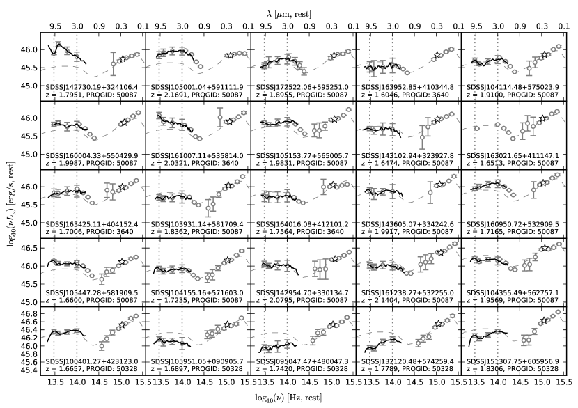
Figure 1.— Spectral energy distributions from ultra-violet to mid-infrared for the $z\sim 2$ quasars in our sample. The continuum in the optical/UV region is sampled by the SDSS photometry; near-IR/optical is sampled by the 2MASS photometry; Spitzer/IRAC photometry samples the downturn of the near-IR bump around $\sim 1.6{\rm{\mu}m}$; Photometric measurements on Spitzer/IRS spectra provides continuum points at 3, 5, 8 and 10 ${\rm{\mu}m}$. Spitzer/IRS mid-infrared spectra smoothed by a 35-point polynomial are shown by the thick dark line. The S/N ratio of the IRS spectrum varies from 10–13 for objects from program 50087, and it is 25–35 for objects from program 50328. The S/N for archival objects from program 3640 is between 6–10. The 3 and 10 ${\rm{\mu}m}$ regions where the graphite dust blackbody, and the silicate features peak, respectively, are indicated with vertical dotted lines. For comparison, we have over-plotted the mean quasar SED from Richards et al. (2006) as a gray dashed line. The mean SED is normalized to the SDSS $i$ band luminosity density. The $i$-band is indicated by an open star symbol. Objects are sorted by their $i$-band luminosities, beginning with least-luminous in top-left corner to most luminous in bottom-right corner.

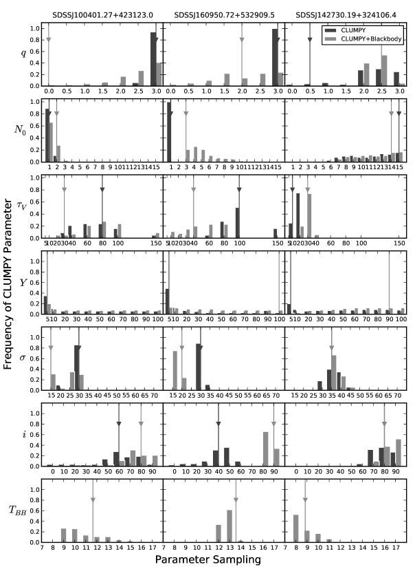
Figure 2.— Distributions of model parameters for three representative sources, SDSSJ100401.27+423123.0, SDSSJ160950.72+532909.5, and SDSSJ142730.19+324106.4, are shown. The distributions are formed from models whose relative error is within 10% of the minimum fitting error of the best fit model. The vertical lines with arrow-heads show the parameter value for the best-fitting model, which is often close to the mode of the parameter distribution for well constrained parameters. Note that radial extent of the torus $Y$, is unconstrained (almost flat distributions), while most other parameters are well constrained. It is interesting that the IR SED of these type 1 quasars (by sample choice) requires high inclination tori, which we think is an artifact of the two-component fitting. The temperature sampling as shown ($T_{BB}$) is in units of 100 K.

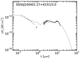
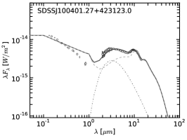
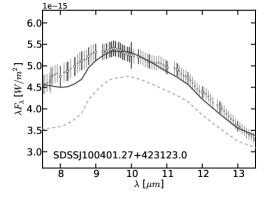
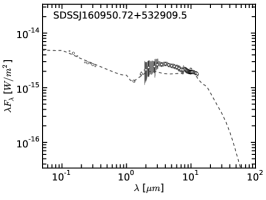
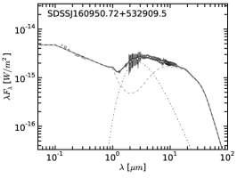
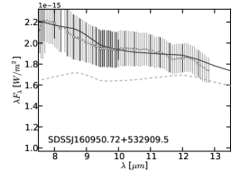
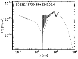
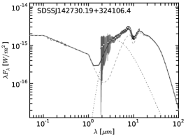
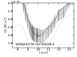
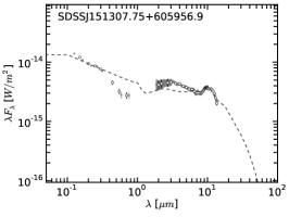
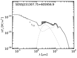
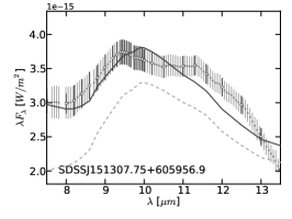
Figure 3.— Best-fitting Clumpy torus models (dashed lines) overlaid on the resampled (open circles with error bars), and original data SEDs (filled gray circles with error bars) and the IRS spectra (clustered gray dots with error bars). Model fits for four sources are shown, SDSSJ100401.27+423123.0, SDSSJ160950.72+532909.5, and SDSSJ142730.19+324106.4, SDSSJ151307.75+605956.9. Panels on the left show fits using only the Clumpy model (dashed line). Note the excess 3 ${\rm{\mu}m}$ emission. Middle panels show fits using a Clumpy model (light gray dashed line), and a hot blackbody component (dash-dotted line) to represent the excess 3 ${\rm{\mu}m}$ emission. The overall fit (dark solid line) improves by incorporating the blackbody component. The panels on the right show a blow up of the 10 ${\rm{\mu}m}$ region from the middle panel. The 10 ${\rm{\mu}m}$ region of SDSSJ151307.75+605956.9 (bottom row, right panel) shows two peaks, one around 9.7 and one around 11.3 ${\rm{\mu}m}$ possibly indicative of crystalline dust species. See Table 6 for values of best fitting parameters.

References

- Antonucci (1993) Antonucci, R. 1993, ARA&A, 31, 473
- Barvainis (1987) Barvainis, R. 1987, ApJ, 320, 537
- Buchanan et al. (2006) Buchanan, C. L., et al. 2006, AJ, 132, 401
- Davidson & Netzer (1979) Davidson, K., & Netzer, H. 1979, Reviews of Modern Physics, 51, 715
- Dullemond & van Bemmel (2005) Dullemond, C. P., & van Bemmel, I. M. 2005, A&A, 436, 47
- Edelson & Malkan (1986) Edelson, R. A., & Malkan, M. A. 1986, ApJ, 308, 59
- Elitzur & Shlosman (2006) Elitzur, M., & Shlosman, I. 2006, ApJ, 648, L101
- Fazio et al. (2004) Fazio, G. G., et al. 2004, ApJS, 154, 10
- Fritz et al. (2006) Fritz, J., Franceschini, A., & Hatziminaoglou, E. 2006, MNRAS, 366, 767
- Gallagher et al. (2007) Gallagher, S. C., et al. 2007, ApJ, 661, 30
- Glikman et al. (2006) Glikman, E., Helfand, D. J., & White, R. L. 2006, ApJ, 640, 579
- Hao et al. (2005) Hao, L., et al. 2005, ApJ, 625, L75
- Hatziminaoglou et al. (2010) Hatziminaoglou, E., et al. 2010, A&A, 518, L33+
- Hewett & Wild (2010) Hewett, P. C., & Wild, V. 2010, MNRAS, 405, 2302
- Higdon et al. (2004) Higdon, S. J. U., et al. 2004, PASP, 116, 975
- Hönig et al. (2006) Hönig, S. F., et al. 2006, A&A, 452, 459
- Ivezić et al. (1999) Ivezić, Ž., Nenkova, M., & Elitzur, M. 1999, ArXiv Astrophysics e-prints
- Jaffe et al. (2004) Jaffe, W., et al. 2004, Nature, 429, 47
- Konigl & Kartje (1994) Konigl, A., & Kartje, J. F. 1994, ApJ, 434, 446
- Krolik & Begelman (1988) Krolik, J. H., & Begelman, M. C. 1988, ApJ, 329, 702
- Laor & Draine (1993) Laor, A., & Draine, B. T. 1993, ApJ, 402, 441
- Levenson et al. (2007) Levenson, N. A., et al. 2007, ApJ, 654, L45
- Little-Marenin & Little (1988) Little-Marenin, I. R., & Little, S. J. 1988, ApJ, 333, 305
- Lonsdale et al. (2003) Lonsdale, C. J., et al. 2003, PASP, 115, 897
- Maiolino et al. (2001) Maiolino, R., Marconi, A., & Oliva, E. 2001, A&A, 365, 37
- Markwick-Kemper et al. (2007) Markwick-Kemper, F., et al. 2007, ApJ, 668, L107
- Mason et al. (2006) Mason, R. E., et al. 2006, ApJ, 640, 612
- Mor et al. (2009) Mor, R., Netzer, H., & Elitzur, M. 2009, ApJ, 705, 298
- Murayama et al. (2000) Murayama, T., Mouri, H., & Taniguchi, Y. 2000, ApJ, 528, 179
- Murray & Chiang (1995) Murray, N., & Chiang, J. 1995, ApJ, 454, L105+
- Nenkova et al. (2002) Nenkova, M., Ivezić, Ž., & Elitzur, M. 2002, ApJ, 570, L9
- Nenkova et al. (2008a) Nenkova, M., et al. 2008a, ApJ, 685, 147
- Nenkova et al. (2008b) Nenkova, M., et al. 2008b, ApJ, 685, 160
- Netzer et al. (2007) Netzer, H., et al. 2007, ApJ, 666, 806
- Neugebauer et al. (1979) Neugebauer, G., et al. 1979, ApJ, 230, 79
- Nikutta et al. (2009) Nikutta, R., Elitzur, M., & Lacy, M. 2009, ApJ, 707, 1550
- Pier & Krolik (1992) Pier, E. A., & Krolik, J. H. 1992, ApJ, 401, 99
- Pier & Krolik (1993) —. 1993, ApJ, 418, 673
- Polletta et al. (2008) Polletta, M., et al. 2008, ApJ, 675, 960
- Proga et al. (2000) Proga, D., Stone, J. M., & Kallman, T. R. 2000, ApJ, 543, 686
- Rees et al. (1969) Rees, M. J., et al. 1969, Nature, 223, 788
- Richards et al. (2003) Richards, G. T., et al. 2003, AJ, 126, 1131
- Richards et al. (2006) Richards, G. T., et al. 2006, ApJS, 166, 470
- Riffel et al. (2009) Riffel, R. A., Storchi-Bergmann, T., & McGregor, P. J. 2009, ApJ, 698, 1767
- Roche & Aitken (1984) Roche, P. F., & Aitken, D. K. 1984, MNRAS, 208, 481
- Rodríguez-Ardila & Mazzalay (2006) Rodríguez-Ardila, A., & Mazzalay, X. 2006, MNRAS, 367, L57
- Rowan-Robinson (1995) Rowan-Robinson, M. 1995, MNRAS, 272, 737
- Sanders et al. (1989) Sanders, D. B., et al. 1989, ApJ, 347, 29
- Schartmann et al. (2005) Schartmann, M., et al. 2005, A&A, 437, 861
- Schartmann et al. (2008) Schartmann, M., et al. 2008, A&A, 482, 67
- Schweitzer et al. (2006) Schweitzer, M., et al. 2006, ApJ, 649, 79
- Shi et al. (2006) Shi, Y., et al. 2006, ApJ, 653, 127
- Siebenmorgen et al. (2005) Siebenmorgen, R., et al. 2005, Astronomische Nachrichten, 326, 556
- Sturm et al. (2005) Sturm, E., et al. 2005, ApJ, 629, L21
- Tristram et al. (2007) Tristram, K. R. W., et al. 2007, A&A, 474, 837
- Urry & Padovani (1995) Urry, C. M., & Padovani, P. 1995, PASP, 107, 803
- Weedman et al. (2005) Weedman, D. W., et al. 2005, ApJ, 633, 706
- Whittet (2003) Whittet, D. C. B., ed. 2003, Dust in the galactic environment
- York et al. (2000) York, D. G., et al. 2000, AJ, 120, 1579