Analytical and Numerical Results on the Positivity of Steady State Solutions of a Thin Film Equation

Abstract.

We consider an equation for a thin-film of fluid on a rotating cylinder and present several new analytical and numerical results on steady state solutions. First, we provide an elementary proof that both weak and classical steady states must be strictly positive so long as the speed of rotation is nonzero. Next, we formulate an iterative spectral algorithm for computing these steady states. Finally, we explore a non-existence inequality for steady state solutions from the recent work of Chugunova, Pugh, & Taranets.

1. Introduction

Thin liquid films appear in a wide range of natural and industrial applications, such as coating processes, and are generically characterized by a small ratio between the thickness of the fluid and the characteristic length scale in the transverse direction. The physics of such processes are reviewed in Oron, Davis & Bankoff,[16] and more recently in Craster & Matar, [13]. If one includes surface tension in the model, the fluid is governed by a degenerate fourth order parabolic equation. Such equations, studied by Bernis & Friedman, [8], Bertozzi & Pugh, [9], and Beretta, Bertsch & dal Passo [7] still hold many challenges. See, for example, [23, 24, 12] for progress on models which include convection, and Becker & Grün,[5], for a thorough review of analytical progress.

There has been recent interest in equations governing the evolution of a thin, viscous film on the outer (or inner) surface of a cylinder of radius $R$ rotating with constant angular velocity $\omega$, as in Figure 1. Subject to non-dimensionalization, this can be modeled by

(1) $$u_{t}+(u^{n}(u_{\theta\theta\theta}+u_{\theta}-\sin\theta)+\omega u)_{\theta}=0,$$

Of particular interest is the case $n=3$, in which one assumes there is no slip at the fluid-cylinder interface. The solution, $u$, measures the (dimensionless) thickness of the fluid, parameterized by the angular variable, $\theta\in\Omega\equiv[-\pi,\pi)$. To derive (1), one begins with the Navier-Stokes equations, together with a kinematic boundary condition for the free surface surface tension. Subject to appropriate physical scalings and geometric symmetries, we are left with a dimensionless equation with just the $\omega$ parameter. We refer the reader to, for instance, [20] and [19] for a full derivation.

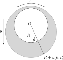
Figure 1. The grey region represents the thin film of liquid on the surface of the cylinder, which is rotating with constant angular velocity $\omega$. We assume symmetry in the $z$ coordinate, so that $u$ is a function of $t$ and $\theta$ only.

Though Buchard, Chugunova, & Stephens,[10], gave a detailed examination of (1) when $\omega=0$, our understanding of the case $\omega\neq 0$ remains incomplete. Some partial results on this case have made assumptions that solutions of (1) are strictly positive, such as in [22], where Pukhnachov proved, under a smallness assumption, positive solutions of (1) exist and are unique.

In this work, we further study steady state solutions – non-negative, time independent solutions $u(\theta)$ of (1), satisfying

(2) $$(u^{n}(u_{\theta\theta\theta}+u_{\theta}-\sin\theta)+\omega u)_{\theta}=0$$

This can be integrated once, to

(3) $$u^{n}(u_{\theta\theta\theta}+u_{\theta}-\sin\theta)+\omega u=q,$$

where $q$, the constant of integration, is the dimensionless flux of the fluid. In particular, we give an elementary proof that when $\omega\neq 0$, both weak and classical solutions must be strictly positive; see Section 2.

For a more extended study of the steady states, it is helpful to explore the problem numerically. This can provide information on how, and if, $u$ and its derivatives develop singularities as the rotation parameter, $\omega$, goes to zero. For such a task, one needs a robust algorithm for computing solutions of (3). In Section 3, we formulate and benchmark an iterative spectral algorithm that is easy to implement and rapidly converges.

Our last result, appearing in Section 4, is motivated by Chugunova, Pugh, & Taranets, [12], who proved that for $n=3$ there can be no positive steady state solutions when the rotation and flux parameters satisfy the inequality

(4) $$q>\left(\tfrac{2}{3}\right)^{3/2}\omega^{3/2}.$$

This was refinement of an earlier bound due to Pukhnachov, [21]. We explore the $(\omega,q)$ phase space and find evidence that this bound may be sharp. Furthermore, it appears that this curve is related to a transition between two different regimes of steady state solutions.

1.1. Notation

In what follows, we shall use the following notational conventions. $C^{k}_{\mathrm{per}}(\Omega)$ is the set of continuous $2\pi$-periodic functions on $\Omega=[-\pi,\pi)$ with $k$ continuous derivatives. $H^{k}_{\mathrm{per}}(\Omega)$ is the set of square integrable $2\pi$-periodic functions on $\Omega=[-\pi,\pi)$ with $k$ square integrable weak derivatives. For a function $\phi$ in one of these spaces, we shall denote its mean by $\bar{\phi}$. For brevity, we will also sometimes write

$$a\lesssim b$$

to indicate that there exists a constant $C>0$ such that

$$a\leq Cb.$$

2. Positivity of Steady States

Here, we prove that both classical and weak steady state solutions of (1) are strictly positive provided $\omega\neq 0$. Buchard, Chugunova, & Stephens, [11], demonstrated that for $\omega=0$, such solutions need not be positive.

2.1. Classical Steady State Solutions

As noted, the case $n=3$ corresponds to a no-slip condition at the surface of the cylinder. With this in mind, it is physically obvious that, as long as $\omega\neq 0$, any steady state solution of (1) with $n=3$ will coat the entire cylinder – that is, there will be no “dry patches” on the surface of the cylinder. The following elementary argument shows that this physical intuition is correct, and is in fact valid for a broad range of exponents $n$.

Proposition 1 (Positivity of Classical Steady State Solutions).

Let $u\in C^{4}_{\mathrm{per}}(\Omega)$ be a classical steady-state solution of (1) with $n>1$. If $\mathrm{supp}\>(u)$ $\neq\Omega$, then $\omega=0$.

Proof.

Assume that $u$ vanishes at $\theta_{0}$. Evaluating (3) at $\theta_{0}$, we have $q=0$. Consequently,

(5) $$u^{n}(u_{\theta\theta\theta}+u_{\theta}-\sin\theta)+\omega u=0.$$

On the support of $u$,

(6) $$u^{n-1}(u_{\theta\theta\theta}+u_{\theta}-\sin\theta)+\omega=0.$$

Since $u_{\theta\theta\theta}$ is bounded as we send $\theta$ towards the root, $\omega=0$. ∎

Though a classical solution of (1) needs to be $C^{4}$, the above proof succeeds without change if $u$ is merely $C^{2}$ with bounded third derivative.

2.2. Weak Steady State Solutions

Positivity can also be proven under weaker assumptions on $u$. We call a non-negative function $u\in H^{2}_{\mathrm{per}}(\Omega)$ a weak solution of(2), if for all $\phi\in C_{\mathrm{per}}^{\infty}(\Omega)$,

(7) $$\int_{-\pi}^{\pi}\!(u^{n}\phi_{\theta})_{\theta}(u_{\theta\theta}+u-\sin(\theta))-\omega u\phi_{\theta}\,d\theta=0.$$

We first establish some pointwise properties of a solution $u$, in the neighborhood of a hypothetical touchdown point, $\theta_{0}$.

Lemma 1.

Let $u\in H^{2}_{\mathrm{per}}(\Omega)$ be non-negative. If there exists $\theta_{0}$ such that $u(\theta_{0})=0$, then

(8a) $$u^{\prime}(\theta_{0})=0$$

(8b) $$u(\theta)=\lvert u(\theta)-u(\theta_{0})\rvert \lesssim\lvert\theta-\theta_{0}\rvert^{3/2},$$

(8c) $$\lvert u^{\prime}(\theta)\rvert=\lvert u^{\prime}(\theta)-u^{\prime}(\theta_{0})\rvert \lesssim\lvert\theta-\theta_{0}\rvert^{1/2}.$$

Proof.

By virtue of a Sobolev embedding theorem in dimension one, $H^{2}\hookrightarrow C^{1,1/2}$, [2, 15]. Therefore, both $u$ and $u^{\prime}$ are Hölder continuous with exponent $1/2$;

(9a) $$\lvert u(\theta)-u(\theta_{0})\rvert \lesssim\lvert\theta-\theta_{0}\rvert^{1/2}$$

(9b) $$\lvert u^{\prime}(\theta)-u^{\prime}(\theta_{0})\rvert \lesssim\lvert\theta-\theta_{0}\rvert^{1/2}.$$

Because $u$ is $C^{1}$ and non-negative, we must have that $u^{\prime}(\theta_{0})=0$ too, otherwise there would be a zero crossing.

Refining (9), we can apply the mean value theorem and the Hölder continuity of $u^{\prime}$ to get

$$\lvert u(\theta)-u(\theta_{0})\rvert=\lvert u^{\prime}(\theta_{\star})\rvert\lvert\theta-\theta_{0}\rvert=\lvert u^{\prime}(\theta_{\star})-u^{\prime}(\theta_{0})\rvert\lvert\theta-\theta_{0}\rvert\lesssim\lvert\theta-\theta_{0}\rvert^{3/2},$$

where $\theta_{\star}$ lies between $\theta$ and $\theta$. ∎

To prove the weak form of Proposition 1, we begin by deriving a weak analog of (3):

Lemma 2.

If $u$ is a weak solution in the sense of (7), then there is a constant $q$, depending only on $u$, such that

(10) $$\int_{-\pi}^{\pi}\!(u^{n}\phi)_{\theta}(u_{\theta\theta}+u-\sin(\theta))-\omega u\phi\,d\theta=q\int_{-\pi}^{\pi}\!\phi\,d\theta$$

for all $\phi\in C_{\mathrm{per}}^{\infty}(\Omega)$.

Proof.

First, observe that for any $\phi\in C_{\mathrm{per}}^{\infty}(\Omega)$, $\phi-\bar{\phi}$ has mean zero and therefore has an antiderivative in $C_{\mathrm{per}}^{\infty}(\Omega)$. Given a test function $\phi$, let $\varphi$ solve $\varphi_{\theta}=\phi-\bar{\phi}$. Plugging in $\varphi$ in (7) in place of $\phi$, we have

(11) $$\int_{-\pi}^{\pi}\!(u^{n}\phi)_{\theta}(u_{\theta\theta}+u-\sin(\theta))-\omega u\phi\,d\theta=\bar{\phi}\int_{-\pi}^{\pi}\!(u^{n})_{\theta}(u_{\theta\theta}+u-\sin(\theta))-\omega u\,d\theta.$$

We may now take

$$q=2\pi\int_{-\pi}^{\pi}\!(u^{n})_{\theta}(u_{\theta\theta}+u-\sin(\theta))-\omega u\,d\theta.$$

∎

We next derive a weak analog of equation (5) in the event that $u$ has a root.

Lemma 3.

For $n>1$, let $u$ be a weak solution satisfying (10) for all $\phi\in C_{\mathrm{per}}^{\infty}(\Omega)$. If $u(\theta_{0})=0$ for some $\theta_{0}\in\Omega$, then $q=0$.

Proof.

Given $\varepsilon>0$, let $\phi\in C_{\mathrm{per}}^{\infty}(\Omega)$ be a compactly supported test function satisfying:

(12) $$0\leq\phi\leq 1,\quad\mathrm{supp}\>\phi\subseteq(-1,+1),\quad\int_{-\pi}^{\pi}\!\phi\,d\theta=1.$$

Let

(13) $$\phi^{\varepsilon}(\theta)\equiv\varepsilon^{-1}\phi((\theta-\theta_{0})/\varepsilon)$$

Then $\mathrm{supp}\>\phi^{\varepsilon}\subseteq I_{\varepsilon}\equiv[\theta_{0}-\varepsilon,\theta_{0}+\varepsilon]$. Substituting $\phi^{\varepsilon}$ into (10), we compute

(14) $$\begin{split}\lvert q\rvert&\leq\lvert\omega\rvert\int_{I_{\varepsilon}}u\phi^{\varepsilon}d\theta+\int_{I_{\varepsilon}}\lvert nu^{n-1}u_{\theta}\phi^{\varepsilon}+u^{n}\phi_{\theta}\rvert\lvert u_{\theta\theta}+u-\sin\theta\rvert d\theta\\ &\leq\lvert\omega\rvert\lVert u\rVert_{L^{\infty}(I_{\varepsilon})}+\lVert nu^{n-1}u_{\theta}\phi^{\varepsilon}+u^{n}\phi^{\varepsilon}_{\theta}\rVert_{L^{2}(I_{\varepsilon})}\lVert u_{\theta\theta}+u-\sin\theta\rVert_{L^{2}(I_{\varepsilon})}\\ &\leq\lvert\omega\rvert\lVert u\rVert_{L^{\infty}(I_{\varepsilon})}+C\sqrt{2\varepsilon}\left(\lVert nu^{n-1}u_{\theta}\phi^{\varepsilon}\rVert_{L^{\infty}(I_{\varepsilon})}+\lVert u^{n}\phi^{\varepsilon}_{\theta}\rVert_{L^{\infty}(I_{\varepsilon})}\right)\end{split}$$

The constant $C$ depends on the $L^{2}$ norms of $u$ and its second derivative, which are both finite by assumption.

Using estimates (8), we have that within $I_{\varepsilon}$,

(15a) $$u^{n}\phi_{\theta}^{\varepsilon} \lesssim\varepsilon^{\frac{3n}{2}-2}$$

(15b) $$nu^{n-1}u_{\theta}\phi^{\varepsilon} \lesssim\varepsilon^{\frac{3n}{2}-2}$$

Substituting this pointwise analysis into (14),

(16) $$\lvert q\rvert\lesssim\varepsilon^{\frac{3}{2}}+\varepsilon^{(3n-3)/2}.$$

Since this holds for all $\varepsilon>0$, we conclude that $q=0$ for $n>1$.

∎

Using Lemmas 2 and 3, we now know that a weak solution with a touchdown satisfies

(17) $$\int_{-\pi}^{\pi}\!(\phi u^{n})_{\theta}(u_{\theta\theta}+u-\sin(\theta))-\omega u\phi\,d\theta=0.$$

Contrast this with its classical counterpart, equation (5).

We now proceed to our main result in the weak case, under the additional restriction that $n\geq 2$:

Proposition 2 (Positivity of Weak Solutions).

Let $u$ be a weak solution satisfying (7) with $n\geq 2$ for all $\varphi\in C_{\mathrm{per}}^{\infty}(\Omega)$. If $S=\{\theta:u(\theta)>0\}\neq\Omega$, then $\omega=0$.

Proof.

The proof is by contradiction. Assuming that $S\neq\Omega$, let $\theta_{0}$ be a point on the boundary of $S$. Given $\varepsilon>0$ sufficiently small, take $y\in\Omega$ such that the interval $I_{\varepsilon/2}\equiv[y-\tfrac{\varepsilon}{2},y+\tfrac{\varepsilon}{2}]$ is contained in $S$ and $|\theta_{0}-y|=\varepsilon$. Now, let $\psi$ be a compactly supported test function as in (12), and let

$$\psi^{\varepsilon}(\theta)=2\varepsilon^{-1}\psi(2(\theta-y)/\varepsilon).$$

This function then has support in $I_{\varepsilon/2}$ as in Figure 2. Finally, define $\phi^{\varepsilon}=\psi^{\varepsilon}/u^{n}$, which is as smooth as $u$, by the conditions on $\varepsilon$ and $y$.

Plugging $\phi^{\varepsilon}$ into (17), we see:

(18) $$\begin{split}\lvert\omega\rvert\int_{I_{\varepsilon/2}}{u}^{1-n}{\psi^{\varepsilon}}d\theta&\leq\int_{I_{\varepsilon/2}}\lvert\psi_{\theta}^{\varepsilon}\rvert\lvert u_{\theta\theta}+u-\cos\theta\rvert d\theta\\ &\leq\lVert\psi_{\theta}^{\varepsilon}\rVert_{L^{2}(I_{\varepsilon/2})}\lVert u_{\theta\theta}+u-\cos\theta\rVert_{L^{2}(I_{\varepsilon/2})}.\end{split}$$

Since ${u}\lesssim\varepsilon^{\frac{3}{2}}$ on the interval and $n>1$, we can bound the integral on the left from below:

(19) $$\int_{I_{\varepsilon/2}}{u}^{1-n}{\psi^{\varepsilon}}d\theta\gtrsim\varepsilon^{\frac{3}{2}(1-n)}.$$

By the construction of $\psi^{\varepsilon}$, $\lVert\psi_{\theta}^{\varepsilon}\rVert_{L^{2}(I_{\varepsilon/2})}\lesssim\varepsilon^{-3/2}$. Therefore,

(20) $$\lvert\omega\rvert\lesssim\varepsilon^{\frac{3}{2}(n-2)}\lVert u_{\theta\theta}+u-\cos\theta\rVert_{L^{2}(I_{\varepsilon/2})}$$

For $n>2$, we immediately observe that since $\varepsilon>0$ is arbitrary, $\omega=0$. For $n=2$, we know that since $(u_{\theta\theta})^{2}$ and $u^{2}$ are measurable,

$$\lVert u_{\theta\theta}+u-\sin\theta\rVert_{L^{2}(I_{\varepsilon/2})}\to 0$$

as $\varepsilon\to 0$, which implies $\omega=0$ in this case.

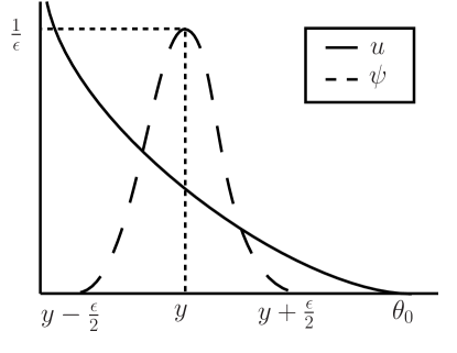
Figure 2. In the proof of proposition 2, we choose a smooth, compactly supported function $\psi$ with support contained in the support of $u$, but close to a zero of $u$.

∎

3. A Computational Method for Steady State Solutions

While we have given a simple proof that when $\omega\neq 0$,steady state solutions must be positive, we have not established their existence. For that, we rely on [22], where it was shown that in the case $n=3$ “small solutions” existed and were unique. Let us motivate this with some heuristic asymptotics. First, assume that $0<q\ll\omega$, i.e.

(21) $$q=\epsilon\omega,\quad 0<\epsilon\ll 1.$$

Subject to this assumption, we may then perform a series expansion in $\epsilon$,

(22) $$u=u^{(0)}+\epsilon u^{(1)}+\epsilon^{2}u^{(2)}+\epsilon^{3}u^{(3)}+\ldots$$

Substituting into

(23) $$u^{3}(u_{\theta\theta\theta}+u_{\theta}-\sin\theta)+\omega u=\epsilon\omega,$$

we then match orders of $\epsilon$. At order $\epsilon^{0}$,

(24) $$(u^{(0)})^{3}(\partial_{\theta}^{n}u^{(0)}+\partial_{\theta}u^{(0)}-\sin\theta)+\omega u^{(0)}=0.$$

As we have no way to solve this, we shall assume the order $\mathrm{O}(\epsilon^{0})$ term is trivial, $u^{(0)}=0$; consequently, $u$ is $\mathrm{O}(\epsilon^{1})$. Proceeding with this assumption, the next few orders are:

(25a) $$\mathrm{O}\left(\epsilon^{1}\right): \quad\omega u^{(1)}=\omega,$$

(25b) $$\mathrm{O}\left(\epsilon^{2}\right): \quad\omega u^{(2)}=0,$$

(25c) $$\mathrm{O}\left(\epsilon^{3}\right): \quad-(u^{(1)})^{3}\sin\theta+\omega u^{(3)}=0.$$

The leading order approximation of the steady state is thus

(26) $$u\approx\frac{q}{\omega}+\frac{1}{\omega}\left(\frac{q}{\omega}\right)^{3}\sin\theta.$$

This corresponds to the “strongly supercritical regime” discussed by Benilov et al.,[3, 6]. A similar analysis applies to the case $n=2$, for which an approximate steady state solution is

(27) $$u\approx\frac{q}{\omega}+\frac{1}{\omega}\left(\frac{q}{\omega}\right)^{2}\sin\theta.$$

This regime was studied in [22], where the expansion was justified by a contraction mapping argument. This motivates the numerical implementation of this approach as a tool for computing such steady states.

3.1. Description of the Algorithm

In what follows, we focus on the case $n=3$, although it can be easily adapted to other cases. We seek to rewrite (3) in the form

$$u=L^{-1}f(u)+g(\theta)$$

where $L$ is a linear operator, $f$ contains the nonlinear terms and $g$ is a a driving term. This will motivate the iteration scheme

$$u^{(j+1)}=L^{-1}f(u^{(j)})+g(\theta)$$

To begin, we divide (3) by $u^{3}$, to obtain

$$(\partial_{\theta}^{3}+\partial_{\theta})u=\sin\theta+qu^{-3}-\omega u^{-2}.$$

As $\partial_{\theta}^{3}+\partial_{\theta}$ has a non trivial kernel, the lefthand side cannot be inverted without careful projection. Pukhnachov resolved this problem by adding and subtracting appropriate terms to the equation. First, we introduce the variable $v$,

$$v\equiv u-\frac{q}{\omega}.$$

Then

(28) $$\begin{split}Lv\equiv(\partial_{\theta}^{3}+\partial_{\theta}+\frac{\omega^{4}}{q^{3}})v&=\sin\theta-\frac{\omega v}{(v+\frac{q}{\omega})^{3}}+\frac{\omega^{4}}{q^{3}}v\\ &=\sin\theta+\frac{\omega^{5}}{q^{3}}v^{2}\frac{3q^{2}+3q\omega v+\omega^{2}v^{2}}{(q+v\omega)^{3}}\equiv\sin\theta+F(v)\end{split}$$

The right hand side of (28) contains a driving term, $\sin\theta$, and an essentially nonlinear term of order $\mathrm{O}(v^{2})$. Rearranging (28),

(29) $$v=\frac{q^{3}}{\omega^{4}}\sin\theta+L^{-1}{F}(v)$$

We now have our iteration scheme

(30) $$v^{(j+1)}=\frac{q^{3}}{\omega^{4}}\sin\theta+L^{-1}{F}(v^{(j)}).$$

In Fourier space, this is

(31) $$\widehat{v}^{(j+1)}_{k}=\frac{q^{3}}{\omega^{4}}\frac{\delta_{k,1}-\delta_{k,-1}}{2i}+\frac{\widehat{F}_{k}^{(j)}}{-ik^{3}+ik+\frac{\omega^{4}}{q^{3}}},\quad F^{(j)}=F(v^{(j)})$$

Plots of solutions computed using this algorithm appear in Figures 3 and 4.

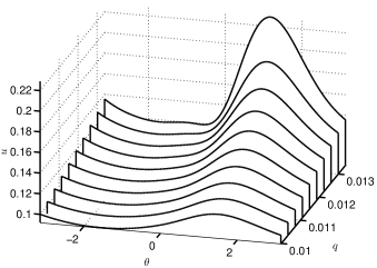
(a) Solutions with fixed $\omega=0.1$

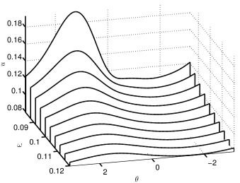
(b) Solutions with fixed $q=0.01$

Figure 3. Steady state solutions with various $\omega$ and $q$ values. Computed by the iterated spectral algorithm at 512 grid points to a tolerance of $10^{-15}$.

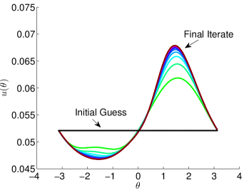
Figure 4. Convergence to a steady state, with $v^{(0)}=0$, $\omega=0.0192$ and $q=0.01$.

3.2. Performance of the Spectral Iterative Method

When our algorithm successfully converges, it does so quite rapidly, as shown in Figure 5, where we plot the error between iterates $v^{(j)}$ and the final iterate. We see that the error is proportional to $e^{-\alpha N}$, although it is clear that the rate, $\alpha$, varies with $q$ and $\omega$. Indeed, as shown in Figure 6, there are choices of these parameters for which our algoirthm diverges; this is consistent with the threshold (4). While this will be further discussed in Section 4, we belive this is closely related to the transition between the “small amplitude regime”, and an essentially nonlinear regime.

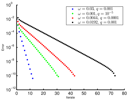
Figure 5. $L^{\infty}$ error between approximate solutions and the final iterate, at 512 grid points, computed to a tolerance of $10^{-10}$.

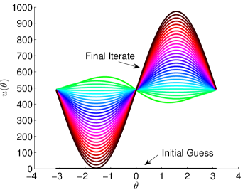
Figure 6. A typical divergent sequence of iterates, caused by the selection of $\omega=0.1$ and $q=0.1$. The iterative spectral method was run to only 30 iterations – after 50 iterations, the solution had a maximum of $4\times 10^{5}$.

However, when we do observe convergence, there is a very high degree of precision, even using a modest number of grid points. Figure 7, shows how quickly the maximum and minimum of the numerical solution converge to one with $10^{5}$ grid points as the number of grid points increases. Again, solutions with values of $q$ and $\omega$ closer to (4) converge less rapidly; the solution in black is much closer to this threshold than the other three.

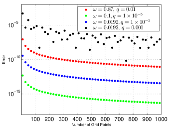
(a) The error in the maximum of the solution.

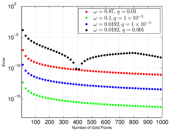
(b) The error in the minimum of the solution.

Figure 7. Convergence of the iterative spectral method, as measured by an error in the minimum and maximum, as the grid size is increased.

3.3. Relation to Other Numerical Methods

Steady state solutions of (1) have been computed in several ways. Some groups, such as Ashmore, Hosoi, & Stone, [3], have run the time dependent equation to steady state. More recently, Benilov, Benilov, & Kopteva computed the solutions directly by a finite difference discretization with a Newton algorithm, [6].

An advantage of our approach is that it converges quickly and is extremely easy to program. An implementation of the algorithm in Matlab is available at http://hdl.handle.net/1807/30015.

Our approach bears some resemblance to Petviashvilli’s algorithm and the related spectral renormalization procedure, which have become quite popular within the nonlinear dispersive wave community for computing solitons, [1, 17, 18]. For such equations, including Korteweg - de Vries and nonlinear Schrödinger/Gross-Pitaevskii, solitary wave solutions solve semilinear elliptic equations of the form

(32) $$-\nabla^{2}Q+\lambda Q=f(Q),\quad\lambda>0,\quad Q:\mathbb{R}^{d}\to\mathbb{R}.$$

For power nonlinearities, $f(Q)=Q^{p}$, Petviashvilli’s algorithm finds a solution by seeking a fixed point of an iteratively renormalized nonlinear equation in the Fourier domain,

(33) $$\widehat{Q}^{(j+1)}=\Lambda_{j}\frac{\widehat{f}(Q^{(j)})}{\lambda+\lvert{\boldsymbol{k}}\rvert^{2}},\quad\Lambda_{j}=\frac{\int(\lambda+\lvert{\boldsymbol{k}}\rvert^{2})\lvert\widehat{Q}^{(j)}\rvert^{2}d{\bf k}}{\int\widehat{f}(Q^{(j)})\overline{\widehat{Q}}^{(j)}d{\bf k}}$$

$Q^{(j)}$ is the $j$-th approximation, and $\Lambda_{j}$ is a renormalization constant at this iterate.

Our scheme, (31) lacked any such renormalization constant, $\Lambda_{j}$. This raises the question of whether or not such a constant could improve our approach. Our results show this is not the case. Introducing the constant

(34) $$\Lambda_{j}\equiv\frac{\sum\left[-ik^{3}+ik+\tfrac{\omega^{4}}{q^{3}}\right]\lvert\widehat{v}_{k}^{(j)}\rvert^{2}}{\sum\widehat{F}_{k}^{(j)}\overline{\widehat{v}}_{k}^{(j)}},$$

we can alter our iteration scheme to be

(35) $$\widehat{v}_{k}^{(j+1)}=\Lambda_{j}^{\gamma}\left(\frac{q^{3}}{\omega^{4}}\frac{\delta_{k,1}-\delta_{k,-1}}{2i}+\frac{\widehat{F}_{k}^{(j)}}{-ik^{3}+ik+\tfrac{\omega^{4}}{q^{3}}}\right).$$

where $\gamma$ is a constant which we may alter to stabilize or accelerate the scheme.

An outcome of our experiments is that not only does our method converge with $\gamma=0$, there does not appear to be appreciable benefit with any other value; see Table 1. For this reason, we do not employ $\Lambda_{j}$, and only deem our algorithm an iterative spectral method.

Table 1. Number of iterations required for $\lVert u_{n+1}-u_{n}\rVert\leq 10^{-10}$i for a variety of initial guesses $u_{0}$. Computed on $2^{12}$ grid points with different values of $\gamma$. $q=0.001153$ and $\omega=0.2$ in all cases.

		$\gamma$
		-0.75	-0.50	-0.25	0	0.25	0.50	0.75
$u_{0}$	$2\frac{q}{\omega}$	42	23	16	12	20	31	69
	$\frac{q}{\omega}+\frac{q^{3}}{\omega^{4}}\cos(\theta)$	2	2	2	2	2	2	2
	$\frac{q}{\omega}+\frac{q^{3}}{\omega^{4}}{\rm sech}(\theta)$	38	18	10	3	9	17	39

3.4. Mass Constraints and Non-Uniqueness

Given values of $q$ and $\omega$, our algorithm successfully converges to non-trivial solutions. However, for a given value of $q$ and $\omega$, there may be more than one solution of (3). To study this phenomenon, it is helpful to introduce the mass of a solution

(36) $$M\equiv\int_{-\pi}^{\pi}u(\theta)d\theta.$$

Benilov, Benilov & Kopteva, [6] tried fixing $\omega$, and numerically explored the relationship between the flux and the mass as they varied. They found non-uniqueness of the solutions, in the sense that for a certain range of $M$, there were multiple solutions with different values of $q$. Alternatively, for a certain range of $q$, there were multiple solutions with different values of $M$. See Figure 14 of their work for a phase diagram, and see our Figure 10 for a similar diagram.

This non-uniqueness affects our algorithm. For a given $(\omega,q)$, the solution that the method converges to may not be the solution we desire, as the following example shows. Using, AUTO, [14], if we seek a solution with $M=1$ and $\omega=.09$, we will obtain the solution pictured in Figure 8 (a). This solution has flux parameter $q=0.0114039$.

Suppose we now fix $\omega=.09$, and continue the solution by lowering the mass. As seen Figure 8 (b), there will be a second solution, with the same $q$, but slightly smaller mass. For $q=0.01140392$, the second solution is at $M=0.912782$ Thus, for a given $(\omega,q)$, there may be multiple solutions, each with a different mass– which solution does the iterative spectral algorithm converge to? As Figure 8 (a) shows, it converges to the solution with the smaller mass. The agreement between the AUTO solution and our method’s solution is quite good; after the AUTO solution is splined onto the regular grid of the spectral solution, the pointwise error is $\mathrm{O}(10^{-7})$.

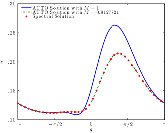
(a) Two different solutions with $\omega=.09$ and $q=0.0114039$

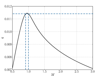
(b) $(M,q)$ pairs of solutions with $\omega=.09$

Figure 8. AUTO finds two solutions by continuation methods the same $\omega$ and $q$, but with different mass. The Spectral Iterative Method converges to the solution with the smaller mass.

The inability of our algorithm to recover the $M=1$ solution can be traced to the development of a linear instability in the iteration scheme. Let $v^{(j)}=v+p^{(j)}$, where $v$ is a solution, and $p^{(j)}$ is a perturbation at iterate $j$. If we linearize (30) about $v$, we have

(37) $$\begin{split}p^{(j+1)}&=L^{-1}\left[\frac{\omega^{5}}{q^{3}}\frac{6q^{3}+6q^{2}\omega v+4q\omega^{2}v^{2}+\omega^{3}v^{3}}{(q+\omega v)^{4}}vp^{(j)}\right]\\ &=L^{-1}\left(F^{\prime}(v)p^{(j)}\right)\equiv\tilde{L}_{v}p^{(j)}.\end{split}$$

If the spectrum of $\tilde{L}_{v}$ lies strictly inside the unit circle, the perturbation will vanish, and the solution $v$ will be stable with respect to the iteration. However, if there are points in the spectrum of this operator which lie outside the unit circle, the solution will be unstable to the iteration, and we would expect our algorithm to diverge.

Though we shall not attempt to prove properties of the spectrum of $\tilde{L}$, we can discretize our problem and compute eigenvalues of the induced matrix. Computing the eigenvalues of a discrete approximation of $\tilde{L}_{v}$ at the two AUTO solutions, we find that the matrix corresponding to the $M=1$ solution does, in fact, have an eigenvalue outside the unit circle, $\lambda_{\rm unstable}=1.017059$; see Figure 9. The discretized operator is defined as

(38) $${\bf\tilde{L}}_{\bf v}\left(D^{3}+D+\tfrac{\omega^{4}}{q^{3}}I\right)^{-1}\mathrm{diag}\left\{F^{\prime}({\bf v})\right\}$$

with the differentiation matrix $D$, a dense Toeplitz matrix for band limited interpolants, as in [25]. The value of the unstable eigenvalue converges quite quickly as we increase the number of grid points, as shown in Table 2.

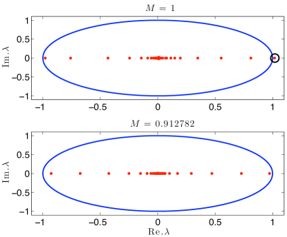
Figure 9. The eigenvalues of the discretized $\tilde{L}_{v}$ for the two solutions computed using AUTO with $\omega=.09$ and $q=.0114039$. Note that for the $M=1$ solution, there is an eigenvalue outside the unit circle at $\lambda=1.017059$. Computed with 2048 grid points.

Table 2. Values of the unstable eigenvalue of ${\bf\tilde{L}}_{\bf v}$ for the $\omega=.09$, $q=.0114039$ and $M=1$ solution as a function of the number of grid points.

No. of Grid Points	$\lambda_{\rm unstable}$
16	1.01711308844
64	1.01705921834
256	1.01705919446
2048	1.01705919124

The $(M,q)$ phase space of solutions with fixed $\omega$ can be more tortuous than that shown in Figure 8 (b). Indeed, as we send $\omega\to 0$, a singular limit, there may not just be multiple solutions of different mass and the same flux, but also multiple solutions of different flux and the same mass. Such an example appears in Figure 10. These cases are more extensively explored in [6] and in Badali et al, [4].

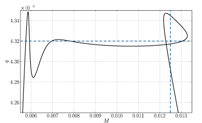
Figure 10. The $(M,q)$ phase space of solutions with rotation parameter $\omega=5\times 10^{-6}$. Note that there can be as many as six solutions of different mass and the same flux, and as many as three solutions of different flux and the same mass. Computed using AUTO.

4. Non-Existence Results

As mentioned in the introduction, in [12], the authors prove that solutions to (3) do not exist for all $(\omega,q)$ pairs. Indeed, they show there are no solutions when (4) holds. Interestingly, this relation is stated entirely in terms of $q$ and $\omega$, and makes no consideration of the mass, $M$.

We now explore, numerically, (4). For fixed mass, we compute the associated solution at a variety of $\omega$ values, determining $q$. The results are appear in Figure 11. As $(\omega,q)$ cannot uniquely determine $u$, we rely on AUTO and its continuation algorithms, rather than our own iterative scheme.

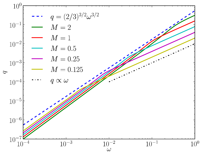
Figure 11. The $(\omega,q)$ phase space of solutions to (3) at prescribed mass values. As the figure shows, even two parameters are insufficient to uniquely determine a steady state solution; where the curves of constant mass cross, there will be two or more solutions with the same $\omega$ and $q$ values. All curves of solutions are constrained by (4), as expected. Also note that at fixed $q$, for sufficiently large $\omega$, the relationship is nearly linear. Computed using AUTO.

Examining the figure, we remark on the two features found in each fixed mass curve. Far to the right of the non-existence line, the $\omega$-$q$ relationship appears to be linear. Indeed, for moderate mass values, the relationship appears to be of the form (21). It is in this “small amplitude” regime that our iterative spectral algorithm succeeds.

As $\omega$ continues to decrease, the scaling changes to accomodate (4), and appears to follow a curve like $q\propto\omega^{\beta}$, for a value of $\beta>3/2$. For all masses, the deviation from (4) is less than an order of magnitude. Thus, there is not an obvious small parameter from which to formulate a series expansion. We also remark that there are many intersections between the curves of constant mass; the lack of uniqueness of a solution for a given $(\omega,q)$ is quite common. As $\omega$ and $q$ approach this essentially nonlinear regime, our algorithm becomes limited. As discussed in the preceding, section unstable eigenvalues can appear, precluding convergence to solutions with a desired mass, and the rate of convergence slows.

Turning to Figure 12, we see the tendency of the solutions to form singularities, vertical asymptotes, as $\omega$ tends towards zero for fixed $q$. These were computed using our spectral iterative algorithm; the asymptotes occurred where the algorithm failed to converge in a reasonable number of iterations. As these figures show, it is possible to get quite close to the theoretical threshold of (4). This suggests that the constraint may be sharp, and this warrants further investigation. Even if the constant is not correct, the scaling appears to be sharp, and the inequality plays an important role in separating two physical regimes.

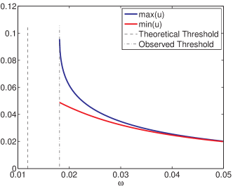
(a) $q=1\times 10^{-3}$. The mass of the final solution was 0.3951

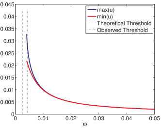
(b) $q=1\times 10^{-4}$. The mass of the final solution was 0.1612

Figure 12. Thickness of solutions with a grid size of $2^{10}$ as $\omega$ is varied. The dashed lines denote the observed threshold at which our spectral iterative algorithm fails and the theoretical threshold, (4) beyond which no solutions should exist. Computed using the spectral iterative method.

5. Discussion

In this work, we have given a simple proof of the positivity of steady state solutions of a thin film equation with rotation, subject to modest assumptions, provided $n\geq 2$. It may be possible to employ additional regularity properties of the steady state solution to lower this threshold; we only relied on Sobolev embeddings in our result.

We have also formulated a very easy to implement algorithm for computing the steady state solutions for a given $(\omega,q$) pair. However, in cases where multiple solutions are known to exist, an instability can develop about one of the solutions, precluding convergence to this solution. We conjecture that the preference is related to the proximity to the non-existence curve, where the parameters have left the small amplitude regime. Finding a way to stabilize the spectral algorithm in this regime remains an open problem.

Finally, our computations suggest further exploration of the non-existence curve is warranted. Figures 11 and 12 suggest that the nonexistence relationship may be sharp. Furthermore, the phase diagram indicates that this inequality separates two physical regimes. In the first, where $\omega$ and $q$ are nearly linearly related, the solution is nearly constant, and can be approximated by (26). In order to accomodate the nonexistence constraint, the phase diagram bends, and we enter a regime where the parameters are nonlinearly related, and the steady state solutions cease to be well described by unimodal bumps.

Acknowledgements: The authors wish to thank A. Buchard and M. Chugunova for suggesting this problem and for many helpful discussions throughout this project’s development. This work was supported in part by NSERC Discovery Grant # 311685-10 and an NSERC Undergraduate Student Research Award.

References

- [1] M. J. Ablowitz and Z. H. Musslimani. Spectral renormalization method for computing self-localized solutions to nonlinear systems. Optics letters, 30(16):2140–2142, 2005.
- [2] R. Adams and J. Fournier. Sobolev Spaces. Academic Press, 2003.
- [3] J. Ashmore, A. Hosoi, and H. Stone. The effect of surface tension on rimming flows in a partially filled rotating cylinder. Journal of Fluid mechanics, 479:65–98, Jan 2003.
- [4] D. Badali, M. Chugunova, and D. Pelinovsky…. Regularized shock solutions in coating flows with small surface tension. Physics of Fluids, 23(9):093103, Jan 2011.
- [5] J. Becker and G. Grün. The thin-film equation: recent advances and some new perspectives. Journal of Physics: Condensed Matter, 17(9):S291–S307, Mar. 2005.
- [6] E. Benilov, M. Benilov, and N. Kopteva. Steady rimming flows with surface tension. Journal of Fluid mechanics, 597:91–118, Jan 2008.
- [7] E. Beretta, M. Bertsch, and R. D. Passo. Nonnegative solutions of a fourth-order nonlinear degenerate parabolic equation. Arch. Rational Mech. Anal., 129(2):175–200, 1995.
- [8] F. Bernis and a. Friedman. Higher order nonlinear degenerate parabolic equations. Journal of Differential Equations, 83(1):179–206, Jan. 1990.
- [9] A. L. Bertozzi and M. C. Pugh. The lubrication approximation for thin viscous films: the moving contact line with a “porous media” cut-off of van der waals interactions. Nonlinearity, 7(6):1535–1564, 1994.
- [10] A. Burchard, M. Chugunova, and B. K. Stephens. Lyapunov’s method proves convergence to equilibrium for a thin film equation. arXiv, math.AP, Nov 2010.
- [11] A. Burchard, M. Chugunova, and B. K. Stephens. On the energy-minimizing steady states of a thin film equation. arXiv, math.AP, Sep 2010. 14 pages, 5 figures.
- [12] M. Chugunova, M. Pugh, and R. Taranets. Nonnegative solutions for a long-wave unstable thin film equation with convection. SIAM Journal on Mathematical Analysis, 42(4):1826–1853, Jan 2010.
- [13] R. Craster and O. Matar. Dynamics and stability of thin liquid films. Reviews of Modern Physics, 81(3):1131–1198, Jan 2009.
- [14] E. Doedel, B. Oldeman, and et al. AUTO-07P.
- [15] L. Evans. Partial Differential Equations, volume 19 of Graduate Studies in Mathematics. American Mathematical Society, 1998.
- [16] A. Oron and S. G. Bankoff. Long-scale evolution of thin liquid films. Reviews of Modern Physics, 69(3):931–980, July 1997.
- [17] D. E. Pelinovsky and Y. Stepanyants. Convergence of petviashvili’s iteration method for numerical approximation of stationary solutions of nonlinear wave equations. SIAM Journal on Numerical Analysis, 42(3):1110–1127, 2005.
- [18] V. Petviashvili. Equation of an extraordinary soliton. Soviet Journal of Plasma Physics, Jan 1976.
- [19] K. Pougatch and I. Frigaard. Thin film flow on the inside surface of a horizontally rotating cylinder: Steady state solutions and their stability. Physics of Fluids, 23(2):022102, Jan 2011.
- [20] V. Pukhnachev. Motion of a liquid film on the surface of a rotating cylinder in a gravitational field. Journal of Applied Mechanics and Technical Physics, 18(3):344–351, 1977.
- [21] V. Pukhnachov. Asymptotic solution of the rotating film problem. Izv. Vyssh. Uchebn. Zaved. Severo-Kavkaz. Reg. Estestv. Nauk, “Mathematics and Continuum Mechanics”(a special issue), pages 191–199, 2004.
- [22] V. Pukhnachov. On the equation of a rotating film. Siberian Mathematical Journal, 46(5):913–924, 2005.
- [23] A. E. Shishkov and R. M. Taranets. On the equation of the flow of thin films with nonlinear convection in multidimensional domains. Ukr. Mat. Visn., 1(3):402–444, 447, 2004.
- [24] R. M. Taranets and A. E. Shishkov. A singular cauchy problem for the equation of the flow of thin viscous films with nonlinear convection. Ukraïn. Mat. Zh., 58(2):250–271, 2006.
- [25] L. Trefethen. Spectral methods in MATLAB, volume 10. SIAM, 2000.