Estimation of means in graphical Gaussian models with symmetries

Abstract

We study the problem of estimability of means in undirected graphical Gaussian models with symmetry restrictions represented by a colored graph. Following on from previous studies, we partition the variables into sets of vertices whose corresponding means are restricted to being identical. We find a necessary and sufficient condition on the partition to ensure equality between the maximum likelihood and least-squares estimators of the mean.

and

1 Introduction

The elegant principles of symmetry and invariance appear in many areas of statistical research [e.g., Dawid (1988), Diaconis (1988), Eaton (1989), Viana (2008)]. Symmetry restrictions in the multivariate Gaussian distribution have a long history [Andersson (1975), Andersson, Brøns and Jensen (1983), Jensen (1988), Olkin (1972), Olkin and Press (1969), Votaw (1948), Wilks (1946)] and have recently been combined with conditional independence relations [Andersen et al. (1995), Højsgaard and Lauritzen (2008), Hylleberg, Jensen and Ørnbøl (1993), Madsen (2000)].

This article is concerned with graphical Gaussian models with symmetry constraints introduced by Højsgaard and Lauritzen (2008). The types of restrictions are: equality between specified elements of the concentration matrix (RCON), equality between specified partial correlations (RCOR) and restrictions generated by permutation symmetry (RCOP), a special instance of the former two. The models can be represented by vertex and edge colored graphs, where parameters associated with equally colored vertices or edges are restricted to being identical.

We consider maximum likelihood estimation of a nonzero mean $\mu$ subject to specific equality constraints, assuming the covariance matrix $\Sigma$ satisfies the restrictions of one of the above models. This could be relevant, for example, if treatment effects are to be estimated in an experiment where the basic error structure in the units exhibits conditional independencies in a symmetric pattern.

For the Gaussian distribution, maximum likelihood estimation of $\mu$ under an unknown covariance structure is generally nontrivial, as the maximizer of the likelihood function in $\mu$ for fixed $\Sigma$ may depend on $\Sigma$. The least-squares estimator $\mu^{*}$, however, is defined by minimizing the sum of squares so that in case of equality of $\hat{\mu}$ and $\mu^{*}$, the former is independent of $\Sigma$. Kruskal (1968) showed that for for fixed $\Sigma$, and $\mu$ in an affine space $\Omega$, $\hat{\mu}$ and $\mu^{*}$ agree if and only if $\Omega$ is stable under $\Sigma$, or equivalently under $K=\Sigma^{-1}$; see also Haberman (1975) and Eaton (1983). Here we derive a necessary and sufficient condition on the graph coloring representing a model and the symmetry constraints on the mean vector $\mu$ which ensures this stability and hence equality of estimators.

We let $G=(V,E)$ denote the dependence graph of the model and let its colored version be denoted by $\mathcal{G}=(\mathcal{V},\mathcal{E})$, where $\mathcal{V}$ denotes a partition of $V$ into vertex color classes and $\mathcal{E}$ a partition of $E$ into edge color classes. The symbol $\mathcal{M}$ is to denote a partition of $V$ such that whenever two vertices are in the same set of $\mathcal{M}$, the corresponding means are restricted to being equal. The necessary and sufficient condition for equality of $\hat{\mu}$ and $\mu^{*}$ in the symmetry model represented by $(\mathcal{V},\mathcal{E})$ is twofold: (i) the partition $\mathcal{M}$ must be finer than $\mathcal{V}$; and (ii) the partition must be equitable with respect to every edge color class in $\mathcal{E}$ as defined by Sachs (1966).

For example, the graph in Figure 1 represents a graphical Gaussian symmetry model for data concerning the head dimensions of first and second sons known as Frets’s heads [Frets (1921), Mardia, Kent and Bibby (1979)]; here $L_{1},B_{1}$ denotes the length and breadth of the head of the first son, and similarly for $L_{2},B_{2}$.

Figure 1: Graphical Gaussian symmetry model supported by Frets’s heads.

This model has previously been found to be well supported by the data [Gehrmann (2011), Højsgaard and Lauritzen (2008), Whittaker (1990)] when no constraints were considered on the means. We may, for example, be interested in the hypothesis that the two lengths have the same mean, and the two breadths have the same mean, indicating that head dimensions do not generally change with the parity of the son. We shall demonstrate that this hypothesis is simple in the sense that the maximum likelihood estimator, or MLE for short, of the mean under this hypothesis can be found by a simple average. Also, we shall demonstrate that this is not the case if we consider lengths and breadths separately.

2 Preliminaries and notation

2.1 Graphical Gaussian models

Let $G=(V,E)$ be an undirected graph with vertex set $V$ and edge set $E$ and let $Y=(Y_{\alpha})_{\alpha\in V}$ be a multivariate Gaussian random vector. Then the graphical Gaussian model represented by $G$ is the set of Gaussian distributions for which $Y_{\alpha}$ is conditionally independent of $Y_{\beta}$ given the remaining variables, denoted $Y_{\alpha}\mathchoice{\mathrel{\hbox to0.0pt{$\displaystyle\perp$\hss}\mkern 4.1mu{\displaystyle\perp}}}{\mathrel{\hbox to0.0pt{$\textstyle\perp$\hss}\mkern 4.1mu{\textstyle\perp}}}{\mathrel{\hbox to0.0pt{$\scriptstyle\perp$\hss}\mkern 4.1mu{\scriptstyle\perp}}}{\mathrel{\hbox to0.0pt{$\scriptscriptstyle\perp$\hss}\mkern 4.1mu{\scriptscriptstyle\perp}}}Y_{\beta}\mid Y_{V\setminus\{\alpha,\beta\}}$, whenever there is no edge between $\alpha$ and $\beta$ in $G$.

For a multivariate Gaussian $\mathcal{N}_{|V|}(\mu,\Sigma)$ distribution with concentration matrix $\Sigma^{-1}=K=(k_{\alpha\beta})_{\alpha,\beta\in V}$, it holds that $Y_{\alpha}\mathchoice{\mathrel{\hbox to0.0pt{$\displaystyle\perp$\hss}\mkern 4.1mu{\displaystyle\perp}}}{\mathrel{\hbox to0.0pt{$\textstyle\perp$\hss}\mkern 4.1mu{\textstyle\perp}}}{\mathrel{\hbox to0.0pt{$\scriptstyle\perp$\hss}\mkern 4.1mu{\scriptstyle\perp}}}{\mathrel{\hbox to0.0pt{$\scriptscriptstyle\perp$\hss}\mkern 4.1mu{\scriptscriptstyle\perp}}}Y_{\beta}\mid Y_{V\setminus\{\alpha,\beta\}}$ if and only if $k_{\alpha\beta}=0$. Thus letting $\mathcal{S}^{+}(G)$ denote the set of symmetric positive definite matrices indexed by $V$ whose $\alpha\beta$-entry is zero whenever $\alpha\beta\notin E$, the graphical Gaussian model represented by $G$ assumes

$$Y\sim\mathcal{N}_{|V|}(\mu,\Sigma),\qquad\mu\in\Omega=\mathbb{R}^{V},\Sigma^{-1}=K\in\mathcal{S}^{+}(G).$$

For further details, see, for example, Lauritzen (1996), Chapter 5.

2.2 Graph coloring

For general graph terminology we refer to Bollobás (1998). Following Højsgaard and Lauritzen (2008) we define the following notation for graph colorings. Let $G=(V,E)$ be an undirected graph. Then a vertex coloring of $G$ is a partition $\mathcal{V}=\{V_{1},\ldots,V_{k}\}$ of $V$, where we refer to $V_{1},\ldots,V_{k}$ as the vertex color classes. Similarly, an edge coloring of $G$ is a partition $\mathcal{E}=\{E_{1},\ldots,E_{l}\}$ of $E$ into $l$ edge color classes $E_{1},\ldots,E_{l}$. We call a color class containing one element a singleton and a partition containing only singletons as elements a singleton partition.

Then $\mathcal{G}=(\mathcal{V},\mathcal{E})$ denotes the colored graph with vertex coloring $\mathcal{V}$ and edge coloring $\mathcal{E}$; we also say that $(\mathcal{V},\mathcal{E})$ is a graph coloring. We indicate the color class of a vertex by the number of asterisks we place next to it. Similarly we indicate the color class of an edge by dashes. color classes which are singletons are displayed in black and without asterisks or dashes.

2.3 Further notation

As we shall be considering constraints on the mean vector defined by partitions of the mean vector into groups of equal entries, we introduce the following notation. For $\mathcal{M}$ a partition of $V$ and $\alpha,\beta\in V$, we write $\alpha\equiv\beta(\mathcal{M})$ to denote that $\alpha$ and $\beta$ lie in the same set in $\mathcal{M}$ and let $\Omega(\mathcal{M})$ be the linear space of vectors which are constant on each set of the partition $\mathcal{M}$:

$$\Omega(\mathcal{M})=\{(x_{\alpha})_{\alpha\in V}\in\mathbb{R}^{V}\dvtx x_{\alpha}=x_{\beta}\mbox{ whenever }\alpha\equiv\beta(\mathcal{M})\}.$$ (1)

For two partitions $\mathcal{M}_{1}$ and $\mathcal{M}_{2}$ of the same set, we shall say that $\mathcal{M}_{1}$ is finer than $\mathcal{M}_{2}$, denoted by $\mathcal{M}_{1}\leq\mathcal{M}_{2}$, if every set in $\mathcal{M}_{2}$ can be expressed as a union of sets in $\mathcal{M}_{1}$. We equivalently say that $\mathcal{M}_{2}$ is coarser than $\mathcal{M}_{1}$.

If $A$ is a set of edges in a graph $G$, for $\alpha\in V$ we shall write $\operatorname{ne}_{A}(\alpha)$ to denote the set of vertices which are connected to $\alpha$ by an edge inside $A$.

We further adopt the following notation from Højsgaard and Lauritzen (2008). For a colored graph $\mathcal{G}=(\mathcal{V},\mathcal{E})$ and $u\in\mathcal{V}$ we let $T^{u}$ denote the $|V|\times|V|$ diagonal matrix with $T^{u}_{\alpha\alpha}=1$ if $\alpha\in u$ and 0 otherwise. Similarly, for each edge color class $u\in\mathcal{E}$ we let $T^{u}$ be the $|V|\times|V|$ symmetric matrix with $T^{u}_{\alpha\beta}=1$ if $\{\alpha,\beta\}\in u$ and 0 otherwise.

3 Maximum likelihood and least-squares estimation

Letting $K=\Sigma^{-1}$ as above, the density of $Y\sim\mathcal{N}_{|V|}(\mu,\Sigma)$ is given by

$$f_{\mu,K}(y)=\frac{\det K^{1/2}}{(2\pi)^{{|V|/2}}}\exp\{-(y-\mu)^{T}K(y-\mu)/2\}$$

so that the likelihood function based on a sample $\mathcal{Y}=(Y^{i})_{1\leq i\leq n}$ where $Y^{i}$ are independent, and $Y^{i}\sim\mathcal{N}_{|V|}(\mu,\Sigma)$ becomes

$$L(\mu,K;y)\propto\det K^{n/2}\exp\biggl{\{}-\sum_{1\leq i\leq n}(y^{i}-\mu)^{T}K(y^{i}-\mu)/2\biggr{\}}.$$ (2)

If $\mu$ is unrestricted, so that $\mu\in\Omega=\mathbb{R}^{V}$, the likelihood function $L$ in (2) is maximized over $\mu$ for fixed $K$ by the least squares estimator $\mu^{*}=\bar{y}$, and inference about $K$ can be based on the profile likelihood function

$$L(\hat{\mu},K;y)\propto\det K^{n/2}\exp\{-\operatorname{tr}(KW)/2\},$$ (3)

where $W=\sum_{i=1}^{n}(y^{i}-\mu^{*})(y^{i}-\mu^{*})^{T}$ is the matrix of sums of squares and products of the residuals. However, inference about $\mu$ when $K$ is unknown and needs to be estimated is generally not possible, a classic example being known as the Behrens–Fisher problem [see Scheffé (1944) and Drton (2008)], where $\Sigma$ is bivariate and diagonal whereas the mean vector satisfies the restriction $\mu_{1}=\mu_{2}$.

Kruskal (1968) found the following necessary and sufficient condition for the two estimators to agree for fixed $\Sigma$:

Theorem 1 ((Kruskal))

Let $Y$ be a random vector in an inner product space with unknown mean $\mu$ in a linear space $\Omega$ and known covariance matrix $\Sigma$. Then the estimators $\mu^{*}$ and $\hat{\mu}$ coincide if and only if $\Omega$ is invariant under $K=\Sigma^{-1}$, that is, if and only if

$$K\Omega\subseteq\Omega.$$ (4)

Consequently, if (4) is satisfied by all $K$ in a model, the likelihood function can be maximized for fixed $K$ by $\mu^{*}$, and inference on $K$ can be based on the profile likelihood (3).

4 Model types

4.1 Descriptions

As stated earlier, we consider three model types introduced in Højsgaard and Lauritzen (2008), which can be represented by colored graphs. These are discussed briefly here, and we refer to Højsgaard and Lauritzen (2008) for further details.

RCON models: Restrictions on concentrations

RCON models placeequality constraints on the concentration matrix $K$. They restrict off-diagonal elements of $K$ separately from those on the diagonal, so that the restrictions can be represented by a graph coloring $(\mathcal{V},\mathcal{E})$ of $G$, with $\mathcal{V}$ representing the diagonal and $\mathcal{E}$ the off-diagonal constraints. The corresponding set of positive definite matrices is denoted by $\mathcal{S}^{+}(\mathcal{V},\mathcal{E})$.

RCOR models: Restrictions on partial correlations

RCOR models combine equality restrictions on the diagonal of $K$ with equality constraints on partial correlations, given by

$$\rho_{\alpha\beta|V\setminus\{\alpha,\beta\}}=-\frac{k_{\alpha\beta}}{\sqrt{k_{\alpha\alpha}k_{\beta\beta}}},\qquad\alpha,\beta\in V,\alpha\not=\beta.$$ (5)

Constraints of RCOR models may also be represented by a graph coloring $(\mathcal{V},\mathcal{E})$, and we denote the corresponding set of positive definite matrices by $\mathcal{R}^{+}(\mathcal{V},\mathcal{E})$.

RCOP models: Permutation symmetry

RCOP models are determined by distribution invariance under a group of permutations of the vertices which preserve the edges of the graph, that is, a subgroup of $\operatorname{Aut}(G)$, the group of automorphisms of $G$. For $\sigma\in\operatorname{Aut}(G)$, let $G(\sigma)$ be the permutation matrix representing $\sigma$, with $G(\sigma)_{\alpha\beta}=1$ if and only if $\sigma$ maps $\beta$ to $\alpha$, for $\alpha,\beta\in V$. Then a Gaussian $\mathcal{N}_{|V|}(0,\Sigma)$ distribution is preserved by $\sigma$ if and only if

$$G(\sigma)KG(\sigma)^{-1}=K.$$ (6)

The RCOP model generated by a group $\Gamma\subseteq\operatorname{Aut}(G)$ assumes

$$K\in\mathcal{S}^{+}(G,\Gamma)=\mathcal{S}^{+}(G)\cap\mathcal{S}^{+}(\Gamma),$$

where $\mathcal{S}^{+}(\Gamma)$ denotes the set of positive definite matrices satisfying (6) for all $\sigma\in\Gamma$ [Højsgaard and Lauritzen (2008)].

4.2 Relations between model types

Under certain conditions on the coloring, RCON and RCOR models, which are determined by the same colored graph, coincide in their model restrictions. First we define edge regularity of a graph coloring.

Definition 1.

Let $\mathcal{G}=(\mathcal{V},\mathcal{E})$ be a colored graph. We say that $(\mathcal{V},\mathcal{E})$ is edge regular if any pair of edges in the same color class in $\mathcal{E}$ connects the same vertex color classes.

The relevant result in Højsgaard and Lauritzen (2008) then becomes:

Proposition 1.

The RCON and RCOR models, that are determined by the colored graph $\mathcal{G}=(\mathcal{V},\mathcal{E})$, yield identical restrictions, that is,

$$\mathcal{S}^{+}(\mathcal{V},\mathcal{E})=\mathcal{R}^{+}(\mathcal{V},\mathcal{E})$$

if and only if $(\mathcal{V},\mathcal{E})$ is edge regular.

RCOP models fall into the class of models which satisfy the condition in Proposition 1, as we show below:

Proposition 2.

If a colored graph $\mathcal{G}=(\mathcal{V},\mathcal{E})$ represents an RCOP model, then $(\mathcal{V},\mathcal{E})$ is edge regular.

Let $\mathcal{G}=(\mathcal{V},\mathcal{E})$ represent an RCOP model, generated by permutation group $\Gamma\subseteq\operatorname{Aut}(G)$, say, and let $u\in\mathcal{E}$ and $e,f\in u$. By definition, there exists $\sigma\in\Gamma$ mapping $e$ to $f$ while leaving $(\mathcal{V},\mathcal{E})$ invariant. This implies that the colorings of the end vertices of $e$ and $f$ must be identical.

Thus, if for a graph $G=(V,E)$ we let $\mathcal{V}$ and $\mathcal{E}$ denote the vertex orbits and edge orbits of a group $\Gamma\subseteq\operatorname{Aut}(G)$, then $\mathcal{S}^{+}(G,\Gamma)=\mathcal{S}^{+}(\mathcal{V},\mathcal{E})=\mathcal{R}^{+}(\mathcal{V},\mathcal{E})$ [Højsgaard and Lauritzen (2008)].

For example, since the coloring of the graph in Figure 1 is generated by the group $\Gamma=\{I,\sigma\}$ with $\sigma$ simultaneously permuting $B_{1}$ with $B_{2}$ and $L_{1}$ with $L_{2}$, the corresponding two sets $\mathcal{S}^{+}(\mathcal{V},\mathcal{E})$ and $\mathcal{R}^{+}(\mathcal{V},\mathcal{E})$ coincide.

5 Equality of maximum likelihood and least-squares estimator

By Theorem 1, the maximum likelihood estimator $\hat{\mu}$ and least-squares estimator $\mu^{*}$ agree for $\mu$ in a linear subspace $\Omega\subseteq\mathbb{R}^{V}$ if and only if $\Omega$ is stable under all $K$ in the model. Below we show that for RCON and RCOR models, and thus also for RCOP models, invariance of $\Omega$ under $K$ is equivalent to invariance under $\{T^{u}\}_{u\in\mathcal{V}\cup\mathcal{E}}$.

Proposition 3.

Let $\mathcal{G}=(\mathcal{V},\mathcal{E})$ be a colored graph representing the RCON model with $K\in\mathcal{S}^{+}(\mathcal{V},\mathcal{E})$. Then for $\Omega\subseteq\mathbb{R}^{V}$,

$$K\Omega\subseteq\Omega\qquad\forall K\in\mathcal{S}^{+}(\mathcal{V},\mathcal{E})\quad\Longleftrightarrow\quad T^{u}\Omega\subseteq\Omega\qquad\forall u\in\mathcal{V}\cup\mathcal{E}.$$

By definition of RCON models, all $K\in\mathcal{S}^{+}(\mathcal{V},\mathcal{E})$ can be written as

$$K=\sum_{u\in\mathcal{V}\cup\mathcal{E}}\theta_{u}T^{u},\qquad\theta_{u}\in\mathbb{R}\mbox{ for }u\in\mathcal{V}\cup\mathcal{E}$$ (7)

with $\{\theta_{u}\}_{u\in\mathcal{V}\cup\mathcal{E}}$ such that the expression in (7) is positive definite. Suppose first that we have

$$T^{u}\Omega\subseteq\Omega\qquad\forall u\in\mathcal{V}\cup\mathcal{E}.$$

Since $\Omega$ is a linear space this implies invariance under all $K\in\mathcal{S}^{+}(\mathcal{V},\mathcal{E})$.

Next suppose $K\Omega\subseteq\Omega$ for all $K\in\mathcal{S}^{+}(\mathcal{V},\mathcal{E})$. $\mathcal{S}^{+}(\mathcal{V},\mathcal{E})$ is an open convex cone, so that for all $K\in\mathcal{S}^{+}(\mathcal{V},\mathcal{E})$ and $u\in\mathcal{V}\cup\mathcal{E}$ there exists $\lambda_{u}\in\mathbb{R}\setminus\{0\}$ such that

$$K_{u}=K+\lambda_{u}T^{u}\in\mathcal{S}^{+}(\mathcal{V},\mathcal{E}).$$

By assumption, $K\Omega\subseteq\Omega$ and $K_{u}\Omega\subseteq\Omega$, which gives

$$(K_{u}-K)\Omega=\lambda_{u}T^{u}\Omega\subseteq\Omega$$

and thus the desired result.

Although the cone $\mathcal{R}^{+}(\mathcal{V},\mathcal{E})$ is not in general convex, the same holds for RCOR models, as shown below.

Proposition 4.

Let $\mathcal{G}=(\mathcal{V},\mathcal{E})$ be a colored graph. Then for $\Omega\subseteq\mathbb{R}^{V}$,

$$K\Omega\subseteq\Omega\qquad\forall K\in\mathcal{R}^{+}(\mathcal{V},\mathcal{E})\quad\Longleftrightarrow\quad T^{u}\Omega\subseteq\Omega\qquad\forall u\in\mathcal{V}\cup\mathcal{E}.$$

Let $A=(a_{\alpha\beta})_{\alpha,\beta\in V}$ denote the diagonal matrix with entries equal to the inverse partial standard deviations, that is,

$$a_{\alpha\alpha}=\sqrt{k_{\alpha\alpha}}\qquad\mbox{for }\alpha\in V,$$

and let $C=(c_{\alpha\beta})_{\alpha,\beta\in V}$ have all diagonal entries equal to 1 and all off-diagonal entries be given by the negative partial correlations $-\rho_{\alpha\beta|V\setminus\{\alpha,\beta\}}$. Then, by (5), all $K\in\mathcal{R}^{+}(\mathcal{V},\mathcal{E})$ can be uniquely expressed as

$$K=ACA=\sum_{v,w\in\mathcal{V}}a_{v}a_{w}T^{v}T^{w}+\sum_{v,w\in\mathcal{V},u\in\mathcal{E}}c_{u}a_{v}a_{w}T^{v}T^{u}T^{w},$$ (8)

where for $v\in\mathcal{V}$ and $u\in\mathcal{E}$, we let $a_{v}$ and $c_{u}$ denote $a_{\alpha\alpha}$, $\alpha\in v$ and $c_{\alpha\beta}$, $\alpha\beta\in u$, respectively. As for $v,w\in\mathcal{V}$, $T^{v}T^{w}$ is zero unless $v=w$, when it equals $T^{v}$, and equation (8) simplifies to

$$K=\sum_{v\in\mathcal{V}}a_{v}^{2}T^{v}+\sum_{v,w\in\mathcal{V},u\in\mathcal{E}}c_{u}a_{v}a_{w}T^{v}T^{u}T^{w}.$$ (9)

Suppose first that we have

$$T^{u}\Omega\subseteq\Omega\qquad\forall u\in\mathcal{V}\cup\mathcal{E}.$$

As before, since $\Omega$ is a linear space, (9) implies invariance under all $K\in\mathcal{R}^{+}(\mathcal{V},\mathcal{E})$. So suppose $K\Omega\subseteq\Omega$ for all $K\in\mathcal{R}^{+}(\mathcal{V},\mathcal{E})$. Then, in particular, $\Omega$ is invariant under all $K$ of the form

$$K=ACA\qquad\mbox{with $A=\sigma^{2}I$ and $C$ as specified above},$$

represented by the graph coloring $(\{V\},\mathcal{E})$, which has the same edge coloring as $(\mathcal{V},\mathcal{E})$, but with all vertices of the same color. This graph coloring is clearly edge regular (as all edges connect the only vertex color class back to itself), which gives that the represented model is also of type RCON. We may therefore apply Proposition 3, giving

$$T^{u}\Omega\subseteq\Omega\qquad\forall u\in\mathcal{E}.$$

For the vertex coloring, consider the submodel

$$K=ACA\qquad\mbox{with $A$ as specified above and $C=I$}.$$

This submodel is represented by the independence graph with no edges and vertex coloring $\mathcal{V}$, which is also edge regular, so that by Proposition 3,

$$T^{v}\Omega\subseteq\Omega\qquad\forall v\in\mathcal{V},$$

completing the proof.

5.1 Equality restrictions in the means of RCON and RCOR models

Let $\mathcal{M}$ be a partition of $V$ and consider $\Omega(\mathcal{M})$ as in (1). In the following we derive a necessary and sufficient condition on $\mathcal{M}$ and $(\mathcal{V},\mathcal{E})$ for $\Omega(\mathcal{M})$ to be invariant under all $K\in\mathcal{S}^{+}(\mathcal{V},\mathcal{E})$ or all $K\in\mathcal{R}^{+}(\mathcal{V},\mathcal{E})$. By Propositions 3 and 4 we may consider vertex and edge color classes of the colored graph representing the model separately. We begin with the vertex coloring.

Proposition 5.

Let $\mathcal{M}$ and $\mathcal{V}$ be partitions of $V$. Then $\Omega(\mathcal{M})$ is invariant under $\{T^{v}\}_{v\in\mathcal{V}}$ if and only if $\mathcal{M}\leq\mathcal{V}$.

The action of $T^{v}$ for $v\in\mathcal{V}$ on $\mu\in\mathbb{R}^{V}$ is given as

$$T^{v}\mu=\cases{\mu_{\alpha}&\quad if $\alpha\in v$,\cr 0&\quad otherwise.}$$

Let $\mu\in\Omega(\mathcal{M})$, and suppose that $T^{v}\Omega(\mathcal{M})\subseteq\Omega(\mathcal{M})$ for all $v\in\mathcal{V}$. In order for $T^{v}\mu\in\Omega(\mathcal{M})$ for all $v\in\mathcal{V}$, we must have $\alpha\equiv\beta(\mathcal{V})$ whenever $\alpha\equiv\beta(\mathcal{M})$, or equivalently $\mathcal{M}\leq\mathcal{V}$. Conversely, suppose $\mathcal{M}\leq\mathcal{V}$. Then $\alpha\equiv\beta(\mathcal{V})$ whenever $\alpha\equiv\beta(\mathcal{M})$, which gives $T^{v}\mu\in\Omega(\mathcal{M})$ for all $v\in\mathcal{V}$.

Note that the above result implies that the likelihood cannot be maximized in $\mu$ independently of the value of $K$ in the Behrens–Fisher setting, which is the RCON and RCOR model on two variables specified by $\mathcal{V}=\{\{1\},\{2\}\}$, $\mathcal{E}=\varnothing$ together with the restriction $\mu_{1}=\mu_{2}$ on the means, as the mean partitioning is then coarser than the vertex coloring.

Also, for the model of Frets’s heads in Figure 1, the MLE of the mean is not simple if we, for example, wish to estimate the mean under the hypothesis that the heads tend to be square-shaped, that is, if mean lengths are equal to mean breadths, as this partition would not be finer than the vertex coloring.

For the edge coloring, we require the concept of an equitable partition, first defined by Sachs (1966).

Definition 2 ((Sachs)).

Let $G=(V,E)$ be an undirected graph. Then a partition, or equivalent coloring, $\mathcal{V}$ of $V$ is called equitable with respect to $G$ if for all $v\in\mathcal{V}$, $\alpha,\beta\in v$,

$$|\operatorname{ne}_{E}(\alpha)\cap w|=|\operatorname{ne}_{E}(\beta)\cap w|\qquad\forall w\in\mathcal{V}.$$

Chan and Godsil (1997) proved the following.

Proposition 6 ((Chan and Godsil)).

Let $G=(V,E)$ be an undirected graph with adjacency matrix $T$, and let $\mathcal{M}$ be a partition of $V$. Then $\Omega(\mathcal{M})$ is invariant under $T$ if and only if $\mathcal{M}$ is equitable with respect to $G$.

The notion of an equitable partition for vertex colored graphs can be naturally extended to graphs with colored vertices and edges. We term the corresponding graph colorings vertex regular, defined below.

Definition 3.

Let $\mathcal{G}=(\mathcal{V},\mathcal{E})$ be a colored graph, and let the subgraph induced by the edge color class $u\in\mathcal{E}$ be denoted by $G^{u}=(V,u)$. We say that $(\mathcal{V},\mathcal{E})$ is vertex regular if $\mathcal{V}$ is equitable with respect to $G^{u}$ for all $u\in\mathcal{E}$.

Combining Definition 3 with Proposition 6 yields vertex regularity to be a necessary and sufficient condition for $\Omega(\mathcal{M})$ to be invariant under $\{T^{u}\}_{u\in\mathcal{E}}$:

Proposition 7.

For $\mathcal{G}=(\mathcal{V},\mathcal{E})$ a colored graph and $\mathcal{M}$ a partition of $V$, $\Omega(\mathcal{M})$ is invariant under $\{T^{u}\}_{u\in\mathcal{E}}$ if and only if $(\mathcal{M},\mathcal{E})$ is vertex regular.

For $u\in\mathcal{E}$, $T^{u}$ is the adjacency matrix of $G^{u}$. By Proposition 6, $\Omega(\mathcal{M})$ is stable under $\{T^{u}\}_{u\in\mathcal{E}}$ if and only if $\mathcal{M}$ is equitable with respect to $G^{u}$ for all $u\in\mathcal{E}$, or equivalently if and only if $(\mathcal{M},\mathcal{E})$ is vertex regular.

For the Frets’s heads model in Figure 1, this implies that restricting the mean breadths and mean lengths on their own does not ensure $\hat{\mu}=\mu^{*}$, as the corresponding partitions $\mathcal{M}=\{\{B_{1},B_{2}\},\{L_{1}\},\{L_{2}\}\}$ and $\mathcal{M}=\{\{B_{1}\},\{B_{2}\},\{L_{1},L_{2}\}\}$ do not give rise to vertex regular colorings $(\mathcal{M},\mathcal{E})$.

Combining Proposition 5 and Proposition 7 establishes our main result:

Theorem 2

Let $\mathcal{G}=(\mathcal{V},\mathcal{E})$ be a colored graph, let $\mathcal{M}$ be a partition of $V$ and consider a sample from a multivariate Gaussian $\mathcal{N}_{|V|}(\mu,\Sigma)$ distribution with $\mu\in\Omega(\mathcal{M})$ and $K=\Sigma^{-1}\in\mathcal{S}^{+}(\mathcal{V},\mathcal{E})$, both unknown. It then holds that

$$\hat{\mu}=\mu^{*}\quad\Longleftrightarrow\quad\mathcal{M}\leq\mathcal{V}\quad\mbox{and}\quad(\mathcal{M},\mathcal{E})\mbox{ is vertex regular.}$$ (10)

The same conclusion holds if $\mathcal{S}^{+}(\mathcal{V},\mathcal{E})$ is replaced by $\mathcal{R}^{+}(\mathcal{V},\mathcal{E})$.

In fact, for any colored graph $\mathcal{G}=(\mathcal{V},\mathcal{E})$ there is always a coarsest partition $\mathcal{M}$ satisfying the conditions in (10) [Gehrmann (2011)]. The finest variant of such a coarsest equitable refinement $\mathcal{M}$ of $\mathcal{V}$ is given by the singleton partition. Clearly it is finer than any vertex coloring, and further naturally gives a vertex regular coloring $(\mathcal{M},\mathcal{E})$. Note that in this case $\Omega(\mathcal{M})$ corresponds to the unrestricted case considered in Section 3, conforming with the fact that then $\hat{\mu}=\mu^{*}$.

5.2 Equality restrictions in the means in RCOP models

The coarsest possible $\mathcal{M}$ for RCON and RCOR models, by (10), is $\mathcal{V}$, for which $\hat{\mu}=\mu^{*}$ if and only if $(\mathcal{V},\mathcal{E})$ is vertex regular. This always holds for RCOP models.

Proposition 8.

If a colored graph $\mathcal{G}=(\mathcal{V},\mathcal{E})$ represents an RCOP model, then $(\mathcal{V},\mathcal{E})$ is vertex regular.

Let $\mathcal{G}=(\mathcal{V},\mathcal{E})$ represent an RCOP model, generated by a subgroup $\Gamma\subseteq\operatorname{Aut}(G)$, say. By Proposition 2, $(\mathcal{V},\mathcal{E})$ is edge regular. Thus whenever two edges $e,f\in E$ are of the same color, they connect the same vertex color classes. Let $\alpha,\beta\in V$ be two equally colored vertices in $\mathcal{V}$. Then, by definition of RCOP models, there exists a permutation $\sigma\in\Gamma$ which maps $\alpha$ to $\beta$ leaving $(\mathcal{V},\mathcal{E})$ invariant. This implies that the degree in each edge color class of $\alpha$ and $\beta$ must be identical. The previous two statements imply

$$|\operatorname{ne}_{u}(\alpha)\cap v|=|\operatorname{ne}_{u}(\beta)\cap v|$$

for all $v\in\mathcal{V}$ and all pairs $\alpha,\beta\in V$ with $\alpha\equiv\beta(\mathcal{V})$, which is precisely the criterion of vertex regularity for the graph coloring $(\mathcal{V},\mathcal{E})$.

We mention in passing that Proposition 2 and Proposition 8 combined establish that colorings of graphs which represent RCOP models are regular in the terminology of Siemons (1983). We conclude from Theorem 2 and Proposition 8:

Corollary 1.

Let $G=(V,E)$ be an undirected graph, and let $(\mathcal{V},\mathcal{E})$ represent the constraints of an RCOP model generated by group $\Gamma\subseteq\operatorname{Aut}(G)$. Then for a sample from a multivariate Gaussian $\mathcal{N}_{|V|}(\mu,\Sigma)$ distribution with $\mu\in\Omega(\mathcal{V})$ and $K=\Sigma^{-1}\in\mathcal{S}^{+}(G,\Gamma)$, both unknown, we always have $\hat{\mu}=\mu^{*}$.

6 Examples

We first consider the example in Figure 1 on head dimensions for first and second sons. Representing an RCOP model, by Proposition 8, the graph in Figure 1 has a vertex regular coloring. It follows from Corollary 1 that the maximum likelihood estimate of the mean under the hypothesis that the mean length and mean breadth are equal for the two sons is simply the total average of the head lengths and the head breadths, respectively. Similarly, it follows from Theorem 2 that the only hypotheses about the mean that have a simple solution are this one and the one where the means are completely unrestricted.

The empirical means of the dimensions $(B_{1},B_{2},L_{1},L_{2})$ are equal to $(151.12,\allowbreak 149.24,185.72,183.84)$, so that the MLE of the means under the hypothesis that the mean lengths and breadths are independent of the parity of the son then become $(150.18,150.18,184.78,184.78)$. The likelihood ratio test is obtained by comparing the maximized profile likelihoods (3) calculated with appropriate residual covariance matrices $W$ under the two hypotheses. Using the R-package gRc [Højsgaard and Lauritzen (2011)] this yields $-2\log\mathrm{LR}=3.27$ on 2 degrees of freedom, so there is no evidence for the sizes depending on the parity of the son.

Our second example is concerned with the examination marks of 88 students in five mathematical subjects [Mardia, Kent and Bibby (1979)]. The RCOP model represented by $\mathcal{G}=(\mathcal{V},\mathcal{E})$ in Figure 2 was demonstrated to be an excellent fit in Højsgaard and Lauritzen (2008).

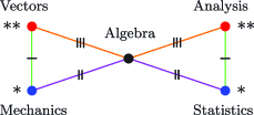
Figure 2: Mathematics marks example.

The model is given by invariance of $K$ under simultaneously permuting Mechanics with Statistics, and Vectors with Analysis. In their fit, Højsgaard and Lauritzen (2008) implicitly assumed an unconstrained mean. The MLE $\hat{\mu}$ is then given by the sample averages $(\hat{\mu}_{\mathrm{al}},\hat{\mu}_{\mathrm{an}},\hat{\mu}_{\mathrm{me}},\hat{\mu}_{\mathrm{st}},\hat{\mu}_{\mathrm{ve}})=(50.60,46.68,\allowbreak 38.96,42.31,50.59)$ in the obvious notation, which corresponds to $\mathcal{M}$ being the singleton partition. However, it could be natural to assume $\mu$ subject to the same invariance as $K$, meaning $\mathcal{M}=\mathcal{V}$, or in this case $\mu_{\mathrm{an}}=\mu_{\mathrm{ve}}$ and $\mu_{\mathrm{me}}=\mu_{\mathrm{st}}$. Then, by Corollary 1, $(\hat{\mu}_{\mathrm{al}},\hat{\mu}_{\mathrm{an}},\hat{\mu}_{\mathrm{me}},\hat{\mu}_{\mathrm{st}},\hat{\mu}_{\mathrm{ve}})=(50.60,48.64,40.63,\allowbreak 40.63,48.64)$. The likelihood ratio statistic for this mean structure relative to the model in Figure 2 with unconstrained mean takes the value of 11.9 on 2 degrees of freedom, and the hypothesis about symmetry in the means is therefore clearly rejected with $p<0.003$.

Note that the sample averages for Vectors and Algebra are almost identical. However, combining the constraints on $K$ represented by the graph in Figure 2 with any hypothesis on the means implying $\mu_{\mathrm{ve}}=\mu_{\mathrm{al}}$ will require joint maximization in $\mu$ and $K$ of the likelihood function in (2) to obtain $\hat{\mu}$.

7 Discussion

The main result of this article is a necessary and sufficient condition on the pattern of equality constraints on the mean vector $\mu$ in a graphical Gaussian symmetry model with colored graph $\mathcal{G}=(\mathcal{V},\mathcal{E})$ which ensures the identity of the least squares estimate $\mu^{*}$ and the maximum likelihood estimate $\hat{\mu}$, given in Theorem 2.

The derived necessary and sufficient condition is formulated in terms of vertex and edge colored graphs and is easily testable, so that any set of equality constraints on $\mu$ together with constraints on either $K$ or the partial correlations can be verified for estimability of $\mu$ by $\mu^{*}$.

The result is, for example, useful if one set of constraints, either on the mean or the independence structure, is assumed to be given and the other may be varied. A setting which falls into this category is the design of experiments seeking to estimate mean treatment effects under the assumption of correlations with inherent symmetries in the error structure at experimental sites. A systematic arrangement of the sites may enforce a symmetry pattern in the concentrations or partial correlations, and thus restrict the concentration matrix as in one of models considered here. Allocation of treatments then effectively restricts the mean response at sites with the same treatment to be identical, and the condition derived can be used to find treatment allocations which ensure estimability of mean treatment effects without knowledge of the value of $\Sigma$.

An interesting question directly emerging from our work is concerned with the exact distributions of likelihood ratio test statistics for hypotheses about the mean in RCON, RCOR and RCOP models. In the examples discussed in this paper we have relied on asymptotic theory to judge the significance of test statistics, but it is likely that their distributions can be derived explicitly, for example when the mean hypothesis is given by the natural symmetry of an RCOP model. Hylleberg, Jensen and Ørnbøl (1993) developed explicit likelihood ratio tests for decomposable mean-zero RCOP models generated by compound symmetry [Votaw (1948)], and it would be interesting to extend these results to models with nonzero means and more general symmetry constraints.

We note that if our condition is not satisfied, we would expect phenomena similar to those in the Behrens–Fisher problem implying the general nonuniqueness of the MLE [Drton (2008)] and the nonexistence of an $\alpha$-similar test of the mean hypothesis [Scheffé (1944)].

References

- Andersen et al. (1995) {bbook}[mr] \bauthor\bsnmAndersen, \bfnmH. H.\binitsH. H., \bauthor\bsnmHøjbjerre, \bfnmM.\binitsM., \bauthor\bsnmSørensen, \bfnmD.\binitsD. and \bauthor\bsnmEriksen, \bfnmP. S.\binitsP. S. (\byear1995). \btitleLinear and Graphical Models for the Multivariate Complex Normal Distribution. \bseriesLecture Notes in Statistics \bvolume101. \bpublisherSpringer, \baddressNew York. \bidmr=1440852 \bptokimsref \endbibitem
- Andersson (1975) {barticle}[mr] \bauthor\bsnmAndersson, \bfnmSteen\binitsS. (\byear1975). \btitleInvariant normal models. \bjournalAnn. Statist. \bvolume3 \bpages132–154. \bidissn=0090-5364, mr=0362703 \bptokimsref \endbibitem
- Andersson, Brøns and Jensen (1983) {barticle}[mr] \bauthor\bsnmAndersson, \bfnmSteen A.\binitsS. A., \bauthor\bsnmBrøns, \bfnmHans K.\binitsH. K. and \bauthor\bsnmJensen, \bfnmSøren Tolver\binitsS. T. (\byear1983). \btitleDistribution of eigenvalues in multivariate statistical analysis. \bjournalAnn. Statist. \bvolume11 \bpages392–415. \biddoi=10.1214/aos/1176346149, issn=0090-5364, mr=0696055 \bptokimsref \endbibitem
- Bollobás (1998) {bbook}[mr] \bauthor\bsnmBollobás, \bfnmBéla\binitsB. (\byear1998). \btitleModern Graph Theory. \bseriesGraduate Texts in Mathematics \bvolume184. \bpublisherSpringer, \baddressNew York. \bidmr=1633290 \bptokimsref \endbibitem
- Chan and Godsil (1997) {bincollection}[mr] \bauthor\bsnmChan, \bfnmAda\binitsA. and \bauthor\bsnmGodsil, \bfnmChris D.\binitsC. D. (\byear1997). \btitleSymmetry and eigenvectors. In \bbooktitleGraph Symmetry (Montreal, PQ, 1996). \bseriesNATO Adv. Sci. Inst. Ser. C Math. Phys. Sci. \bvolume497 \bpages75–106. \bpublisherKluwer Academic, \baddressDordrecht. \bidmr=1468788 \bptokimsref \endbibitem
- Dawid (1988) {barticle}[mr] \bauthor\bsnmDawid, \bfnmA. P.\binitsA. P. (\byear1988). \btitleSymmetry models and hypotheses for structured data layouts. \bjournalJ. Roy. Statist. Soc. Ser. B \bvolume50 \bpages1–34. \bidissn=0035-9246, mr=0954729 \bptnotecheck related\bptokimsref \endbibitem
- Diaconis (1988) {bbook}[mr] \bauthor\bsnmDiaconis, \bfnmPersi\binitsP. (\byear1988). \btitleGroup Representations in Probability and Statistics. \bseriesInstitute of Mathematical Statistics Lecture Notes—Monograph Series \bvolume11. \bpublisherIMS, \baddressHayward, CA. \bidmr=0964069 \bptokimsref \endbibitem
- Drton (2008) {barticle}[mr] \bauthor\bsnmDrton, \bfnmMathias\binitsM. (\byear2008). \btitleMultiple solutions to the likelihood equations in the Behrens–Fisher problem. \bjournalStatist. Probab. Lett. \bvolume78 \bpages3288–3293. \biddoi=10.1016/j.spl.2008.06.012, issn=0167-7152, mr=2479491 \bptokimsref \endbibitem
- Eaton (1983) {bbook}[mr] \bauthor\bsnmEaton, \bfnmMorris L.\binitsM. L. (\byear1983). \btitleMultivariate Statistics: A Vector Space Approach. \bpublisherWiley, \baddressNew York. \bidmr=0716321 \bptokimsref \endbibitem
- Eaton (1989) {bbook}[mr] \bauthor\bsnmEaton, \bfnmM. L.\binitsM. L. (\byear1989). \btitleGroup Invariance Applications in Statistics. \bseriesRegional Conference Series in Probability and Statistics \bvolume1. \bpublisherIMS and American Statistical Association, \baddressHayward, CA and Alexandria, VA. \bidmr=1089423 \bptokimsref \endbibitem
- Frets (1921) {barticle}[author] \bauthor\bsnmFrets, \bfnmG. P.\binitsG. P. (\byear1921). \btitleHeredity of head form in man. \bjournalGenetica \bvolume3 \bpages193–400. \bptokimsref \endbibitem
- Gehrmann (2011) {barticle}[mr] \bauthor\bsnmGehrmann, \bfnmHelene\binitsH. (\byear2011). \btitleLattices of graphical Gaussian models with symmetries. \bjournalSymmetry \bvolume3 \bpages653–679. \biddoi=10.3390/sym3030653, issn=2073-8994, mr=2845303 \bptokimsref \endbibitem
- Haberman (1975) {barticle}[mr] \bauthor\bsnmHaberman, \bfnmShelby J.\binitsS. J. (\byear1975). \btitleHow much do Gauss–Markov and least square estimates differ? A coordinate-free approach. \bjournalAnn. Statist. \bvolume3 \bpages982–990. \bidissn=0090-5364, mr=0378269 \bptokimsref \endbibitem
- Højsgaard and Lauritzen (2008) {barticle}[mr] \bauthor\bsnmHøjsgaard, \bfnmSøren\binitsS. and \bauthor\bsnmLauritzen, \bfnmSteffen L.\binitsS. L. (\byear2008). \btitleGraphical Gaussian models with edge and vertex symmetries. \bjournalJ. R. Stat. Soc. Ser. B Stat. Methodol. \bvolume70 \bpages1005–1027. \biddoi=10.1111/j.1467-9868.2008.00666.x, issn=1369-7412, mr=2530327 \bptokimsref \endbibitem
- Højsgaard and Lauritzen (2011) {bmisc}[author] \bauthor\bsnmHøjsgaard, \bfnmS.\binitsS. and \bauthor\bsnmLauritzen, \bfnmS. L.\binitsS. L. (\byear2011). \bhowpublishedgRc: Inference in graphical Gaussian models with edge and vertex symmetries. R package version 0.3.0. \bptokimsref \endbibitem
- Hylleberg, Jensen and Ørnbøl (1993) {bmisc}[author] \bauthor\bsnmHylleberg, \bfnmB.\binitsB., \bauthor\bsnmJensen, \bfnmM.\binitsM. and \bauthor\bsnmØrnbøl, \bfnmE.\binitsE. (\byear1993). \bhowpublishedGraphical symmetry models. M.Sc. thesis, Aalborg Univ., Aalborg. \bptokimsref \endbibitem
- Jensen (1988) {barticle}[mr] \bauthor\bsnmJensen, \bfnmSøren Tolver\binitsS. T. (\byear1988). \btitleCovariance hypotheses which are linear in both the covariance and the inverse covariance. \bjournalAnn. Statist. \bvolume16 \bpages302–322. \biddoi=10.1214/aos/1176350707, issn=0090-5364, mr=0924873 \bptokimsref \endbibitem
- Kruskal (1968) {barticle}[mr] \bauthor\bsnmKruskal, \bfnmWilliam\binitsW. (\byear1968). \btitleWhen are Gauss–Markov and least squares estimators identical? A coordinate-free approach. \bjournalAnn. Math. Statist \bvolume39 \bpages70–75. \bidissn=0003-4851, mr=0222998 \bptokimsref \endbibitem
- Lauritzen (1996) {bbook}[mr] \bauthor\bsnmLauritzen, \bfnmSteffen L.\binitsS. L. (\byear1996). \btitleGraphical Models. \bseriesOxford Statistical Science Series \bvolume17. \bpublisherClarendon Press, \baddressNew York. \bidmr=1419991 \bptokimsref \endbibitem
- Madsen (2000) {barticle}[mr] \bauthor\bsnmMadsen, \bfnmJesper\binitsJ. (\byear2000). \btitleInvariant normal models with recursive graphical Markov structure. \bjournalAnn. Statist. \bvolume28 \bpages1150–1178. \biddoi=10.1214/aos/1015956711, issn=0090-5364, mr=1810923 \bptokimsref \endbibitem
- Mardia, Kent and Bibby (1979) {bbook}[author] \bauthor\bsnmMardia, \bfnmK. V.\binitsK. V., \bauthor\bsnmKent, \bfnmJ. T.\binitsJ. T. and \bauthor\bsnmBibby, \bfnmJ. M.\binitsJ. M. (\byear1979). \btitleMultivariate Analysis. \bpublisherAcademic Press, \baddressNew York, NY. \bptokimsref \endbibitem
- Olkin (1972) {btechreport}[author] \bauthor\bsnmOlkin, \bfnmI.\binitsI. (\byear1972). \btitleTesting and estimation for structures which are circularly symmetric in blocks. \btypeTechnical report, \binstitutionEducational Testing Service, \baddressPrinceton, NJ. \bptokimsref \endbibitem
- Olkin and Press (1969) {barticle}[mr] \bauthor\bsnmOlkin, \bfnmI.\binitsI. and \bauthor\bsnmPress, \bfnmS. J.\binitsS. J. (\byear1969). \btitleTesting and estimation for a circular stationary model. \bjournalAnn. Math. Statist. \bvolume40 \bpages1358–1373. \bidissn=0003-4851, mr=0245139 \bptokimsref \endbibitem
- Sachs (1966) {barticle}[author] \bauthor\bsnmSachs, \bfnmH.\binitsH. (\byear1966). \btitleÜber Teiler, Faktoren und charakteristische Polynome von Graphen. \bjournalWissenschaftliche Zeitschrift der Technischen Hochschule Ilmenau \bvolume12 \bpages7–12. \bptokimsref \endbibitem
- Scheffé (1944) {barticle}[mr] \bauthor\bsnmScheffé, \bfnmHenry\binitsH. (\byear1944). \btitleA note on the Behrens–Fisher problem. \bjournalAnn. Math. Statist. \bvolume15 \bpages430–432. \bidissn=0003-4851, mr=0011926 \bptokimsref \endbibitem
- Siemons (1983) {barticle}[mr] \bauthor\bsnmSiemons, \bfnmJohannes\binitsJ. (\byear1983). \btitleAutomorphism groups of graphs. \bjournalArch. Math. (Basel) \bvolume41 \bpages379–384. \biddoi=10.1007/BF01371410, issn=0003-889X, mr=0731610 \bptokimsref \endbibitem
- Viana (2008) {bbook}[mr] \bauthor\bsnmViana, \bfnmMarlos A. G.\binitsM. A. G. (\byear2008). \btitleSymmetry Studies: An Introduction to the Analysis of Structured Data in Applications. \bpublisherCambridge Univ. Press, \baddressCambridge. \biddoi=10.1017/CBO9780511755477, mr=2419845 \bptokimsref \endbibitem
- Votaw (1948) {barticle}[mr] \bauthor\bsnmVotaw, \bfnmDavid F.\binitsD. F. Jr. (\byear1948). \btitleTesting compound symmetry in a normal multivariate distribution. \bjournalAnn. Math. Statist. \bvolume19 \bpages447–473. \bidissn=0003-4851, mr=0027999 \bptokimsref \endbibitem
- Whittaker (1990) {bbook}[mr] \bauthor\bsnmWhittaker, \bfnmJoe\binitsJ. (\byear1990). \btitleGraphical Models in Applied Multivariate Statistics. \bpublisherWiley, \baddressChichester. \bidmr=1112133 \bptokimsref \endbibitem
- Wilks (1946) {barticle}[mr] \bauthor\bsnmWilks, \bfnmS. S.\binitsS. S. (\byear1946). \btitleSample criteria for testing equality of means, equality of variances, and equality of covariances in a normal multivariate distribution. \bjournalAnn. Math. Statist. \bvolume17 \bpages257–281. \bidissn=0003-4851, mr=0017498 \bptokimsref \endbibitem