Gravitational and electromagnetic emission by magnetized coalescing binary systems

Abstract

We discuss the possibility to obtain an electromagnetic emission accompanying the gravitational waves emitted in the coalescence of a compact binary system. Motivated by the existence of black hole configurations with open magnetic field lines along the rotation axis, we consider a magnetic dipole in the system, the evolution of which leads to (i) electromagnetic radiation, and (ii) a contribution to the gravitational radiation, the luminosity of both being evaluated. Starting from the observations on magnetars, we impose upper limits for both the electromagnetic emission and the contribution of the magnetic dipole to the gravitational wave emission. Adopting this model for the evolution of neutron star binaries leading to short gamma ray bursts, we compare the correction originated by the electromagnetic field to the gravitational waves emission, finding that they are comparable for particular values of the magnetic field and of the orbital radius of the binary system. Finally we calculate the electromagnetic and gravitational wave energy outputs which result comparable for some values of magnetic field and radius.

Keywords Coalescing binary systems, gravitational waves, electromagnetic emission;

1 Introduction

According to General Relativity, compact binary systems (composed of neutron stars (NS), white dwarfs or black holes (BH)) are strong emitters of gravitational waves (GWs), the ripples of space-time due to the presence of accelerated masses (coalescence). As a consequence of the gradual inspiralling, the system loses energy, linear and angular momentum (Hulse $\&$ Taylor (1975); Nice (2003); Taylor (1989); Stairs (2004); Weisberg $\&$ Taylor (2003)). The coalescence of a compact binary system can be split into three distinct, but not sharply delimited phases: the inspiral, the plunge/mergerand the ring-down. For the inspiral phase an accurate analytical description via the so-called Post-Newtonian (PN) expansion has been developed (for a review see (Blanchet (2006)). Spin and mass quadrupolar contributions to this dynamics are also well-known (Barker $\&$ O’Connell (1975)), with inclusion of leading order spin-orbit (Ryan (1996); Majar $\&$ Vasth (2008); Cornish $\&$ Shapiro Key (2010); Kidder et al. (1993, 1995); O’Connell (2004); Rieth (1997); Will (2005); Zeng $\&$ Will (2007)), spin-spin (Wang $\&$ Will (2007); Arun et al. (2009); Klein $\&$ Jetzer (2010); Apostolatos et al. (1995, 1996); Majar (2009)) and mass quadrupole mass monopole (Poisson (1998); Racine (2008)) couplings.

Similarly to the inspiral, the ring-down phase admits a perturbative analytical model which describes the damped oscillations of the single compact object resulting from the binary coalescence (Berti et al. (2009)). The plunge/merger phase is however non-perturbative, having no analytical description for generic systems, therefore it is studied through numerical simulations.

Templates on binary inspiral (Buonanno $\&$ Damour (1999, 2000); Buonanno et al. (2003); Buonanno $\&$ Damour (2006); Cutler et al. (1993); Damour et al. (1998, 2000); Damour (2001); Damour et al. (2002, 2003); Finn $\&$ Chernoff (1993); Flanagan $\&$ Hughes (1993); Pan et al. (2004)) and robust search algorithms were developed for GWs sources observable with ground-based (LIGO Collaboration (2009); Sengupta (2009); di Serafino et al. (2010); di Serafino $\&$ Riccio (2010)) and space-based interferometers (Arun et al. (2009); Lang $\&$ Hughes (2009)).

In addition to GWs emission, these systems emit electromagnetic radiation(Capozziello et al. (2011, 2010)). This emission is due to dynamics of system and to behavior of plasma around the system. There are many different systems that emit gravitational and electromagnetic waves, and in many case the electromagnetic emission is very energetic (AGNs, QSOs, GRBs).

Pulsars with surface magnetic fields in the range $10^{8\div 12}$ G and magnetars with surface magnetic fields up to $10^{14\div 15}$ G have been reported (Duncan $\&$ Thompson (1992); Sinha $\&$ Mukhopadhyay (2010); Kouveliotou et al. (1998); Thompson $\&$ Duncan (1995); Usov (1992); Vasisht $\&$ Gotthelf (1997); Woods et al. (1999)), as summarized in (Sinha $\&$ Mukhopadhyay (2010)). An upper limit of $10^{18}$ G was also advanced from the requirement to avoid exotic structure in the neutron stars (Sinha $\&$ Mukhopadhyay (2010)). An interaction of the magnetic dipoles modifies the gravitational radiation leaving the system, and hence the back-reaction to the orbit is slightly different. Limits on magnetar magnetic fields render these corrections to the second or even higher PN order. Neutron star binary coalescence, leading to a final black hole with a torus is a configuration believed to be the progenitor of short GRBs. In the black hole-torus central engine part of the torus matter can be converted into radiation, leading to the observed bursts (Belczynski et al. (2008)). Fully general-relativistic simulations of binary neutron star coalescence leading to this configuration have been presented in (Rezzolla et al. (2010)), with a detailed and accurate study of the torus. It was found that unequal mass neutron star binaries led to a larger torus and an empirical formula in terms of the mass ratio and total mass was advanced for the torus mass. Nevertheless, the effects of the magnetic fields were not included in the treatment of Ref. (Rezzolla et al. (2010)). Many efforts are done in order to study the electromagnetic emission from these systems, in particular from a computational point of view. It was showed how the dynamics of the binary systems induce the electromagnetic emission and its link with GWs emission (Palenzuela et al. (2009, 2010); Anderson et al. (2008)).

In this paper we investigate a simple model for the inspiral, which also takes into account the magnetic field. Rather then monitoring the complicated evolution of the individual magnetic momenta of a binary neutron star system, we will introduce a global measure of the electromagnetic properties of the system, given by a single magnetic dipole.

Gravitational radiation transports away energy, linear and orbital angular momentum from the system. While the total angular momentum (defined as the sum of the orbital angular momentum and possible individual spins of the NS) exhibits instantaneous changes during orbital evolution, its secular evolution over timescales larger than the orbital period is a pure decrease in magnitude, with the direction kept fixed (Apostolatos et al. (1994)).

Having in mind (i) the configuration of open field lines aligned with the spin of the final compact object resulting from the coalescence, and (ii) the property of the gravitational radiation to conserve the direction of the total angular momentum on timescales longer than the orbital period, we chose the magnetic field aligned with the total angular momentum of the system.

In Sec. 2, we present an overview on GWs emission from coalescing binary systems. In Sec. 3, we introduce and discuss the magnetic field and we also calculate the correction induced in the GW luminosity and amplitude. For comparison, in Sec. 4, we present the luminosity of the accompanying electromagnetic radiation. These are compared and the conclusions presented in Sec. 5.

2 Gravitational wave emission from coalescing binaries

Let us summarize some basic concepts s of the gravitational radiation generated by the evolution of a compact binary system. A wide discussion about the GWs emission can be found in literature (Maggiore (2007); Misner et al. (1973); Weinberg (1972)). The starting point for any discussion of GWs is the approximation to General Relativity (GR), when the space-time metric can be treated as deviating only slightly from a flat metric (Maggiore (2007); Shapiro $\&$ Teukolsky (1983); Misner et al. (1973)). We start from linearized Einstein equation

$$\square\overline{h}_{\mu\nu}=-\frac{16\pi G}{c^{4}}\,T_{\mu\nu}~{},$$ (1)

where $\Box=\eta_{\mu\nu}\partial^{\mu}\partial^{\nu}$ is the d’Alembertian, expressed in terms of the trace reversed metric perturbation

$$\overline{h}^{\mu\nu}={h}^{\mu\nu}-\frac{1}{2}\eta^{\mu\nu}h~{},$$ (2)

where $h_{\mu\nu}=g_{\mu\nu}-\eta_{\mu\nu}$ and $h=\eta_{\mu\nu}h^{\mu\nu}$ (such that $\overline{h}=-h$). Due to the imposed Lorentz (harmonic) gauge $\partial_{\nu}\overline{h}^{\mu\nu}=0$, only 6 of the 10 components of $h_{\mu\nu}$ are independent. By setting $T_{\mu\nu}=0$ we obtain the vacuum wave equation:

$$\square\overline{h}_{\mu\nu}=0\,.$$ (3)

GWs thus propagate at the speed of light.

We evaluate the leading order contribution to the metric perturbations under the assumption that the internal motions of the source are slow compared to the speed of light. We also assume that the source’s self-gravity is negligible. Let us first introduce the momenta of the mass density

$$M = \frac{1}{c^{2}}\int d^{3}x\,T^{00}(t,\mathbf{x})\,,$$ (4)

$$M^{i} = \frac{1}{c^{2}}\int d^{3}x\,T^{00}(t,\mathbf{x})\,x^{i}\,,$$ (5)

$$M^{ij} = \frac{1}{c^{2}}\int d^{3}x\,T^{00}(t,\mathbf{x})\,x^{i}\,x^{j}~{},$$ (6)

and impose the conservation law $\partial_{\mu}T^{\mu\nu}=0$, valid in linearized gravity. For sources having strong gravitational field, as NSs or BHs, the mass density depends also on the binding energy, however for weak fields and small velocities $T^{00}/c^{2}$ reduces to the rest-mass density $\rho$. Denoting the field $h_{\mu\nu}$ which satisfies the transverse and traceless gauge conditions (Weinberg (1972)), as transverse-traceless tensor $h_{ij}^{TT}$, it is convenient to compute from it explicitly the two indipendent polarization states $h_{+}$ and $h_{\times}$ (Buonanno (2007)).

In terms of the traceless quadrupole tensor

$$Q_{ij}=M_{ij}-\frac{1}{3}\,\delta_{ij}\,\mathcal{M},$$ (7)

($\mathcal{M}$ denoting the trace of $M_{ij}$), the leading order expression of the total radiated power is

$$P=\frac{G}{5c^{5}}\,\langle\dddot{Q}_{ij}\,\dddot{Q}_{ij}\rangle\,.$$ (8)

Henceforth, we will apply this formalism for a compact binary system with masses $m_{1}$ and $m_{2}$, total mass $M=m_{1}+m_{2}$ and reduced mass $\mu=m_{1}\,m_{2}/(m_{1}+m_{2})$. With the plane of motion chosen as the $x$-$y$ plane and in the circular motion approximation the reduced mass particle has the coordinates $\mathbf{r}=\left(x,y,z\right)$ given by

$$x(t)=r\,\cos\omega\,t\,,\quad y(t)=r\,\sin\omega\,t\,,\quad z(t)=0\,,$$ (9)

$r$ being the relative distance between the two bodies. With $\rho=\mu\delta(\mathbf{r})$ we find $M^{ij}=\mu x^{i}\,x^{j}$ with the nontrivial components

$$M_{11} = \frac{1}{2}\,\mu\,r^{2}\,(1+\cos 2\omega t)\,,$$

$$M_{22} = \frac{1}{2}\,\mu\,r^{2}\,(1-\cos 2\omega t)\,,$$

$$M_{12} = \frac{1}{2}\,\mu\,r^{2}\,\sin 2\omega t\,.$$ (10)

From which we obtain

$$h_{+}(t)=\frac{4G}{c^{4}d}\,\mu\,r^{2}\,\omega^{2}\,\frac{(1+\cos^{2}\theta)}{2}\,\cos(2\omega\,t)\,\,,$$ (11)

$$h_{\times}(t)=\frac{4G}{c^{4}d}\,\mu\,r^{2}\,\omega^{2}\,\cos\theta\,\sin(2\omega\,t)\,.$$ (12)

Here the time is shifted in order to eliminate the dependence on $\phi$ (Buonanno (2007)). From Eq. (8) the total radiated power emerges as,

$$P=\frac{32}{5}\,\frac{G\,\mu^{2}\,r^{4}\,\omega^{6}}{c^{5}}\,.$$ (13)

In order to compensate for the loss of energy by GW emission, the radial separation $r$ between the two bodies must decrease. The orbital frequency and consequently the GW frequency also changes in time, and can be derived using from the balance equation

$$\frac{dE_{\mathrm{orbit}}}{dt}=-P\,.$$ (14)

3 Gravitomagnetic corrections on gravitational wave emission

In this section we introduce the magnetic field with the desired structure, namely aligned with the total angular momentum $\mathbf{J}$ of the system.

3.1 Gravitomagnetic-electromagnetic analogy

The gravitomagnetic potential characterizing the compact binary is ${{A_{\mu}}=}\left(0,\mathbf{A}\right)$, with

$$\mathbf{A}={{\alpha\frac{\mathbf{J}\times\mathbf{r}}{{{r^{3}}}}}~{}},$$ (15)

where $\alpha=G/c$ Tartaglia $\&$ Ruggiero (2002), and $\mathbf{r}$ is the separation between the bodies of the binary system. Due to the fact that the motion of the binary system is entirely confined into the orbital plane, we evaluate all the physical quantities of interest in the plane itself. This procedure is analogue to that used in GWs emission calculations, where one reduces the problem only to the planar relative motion. The gravitomagnetic field is found as

$$\mathbf{B}=\mathbf{{\nabla}\times\mathbf{A}}=\frac{2\alpha}{r^{3}}\mathbf{J~{}}.$$ (16)

We have used the assumption, that neutron stars rotate slowly, therefore the proper spin contributions to $\mathbf{J}$ are negligible, also that the relativistic (PN and 2PN corrections) are aligned to the Newtonian orbital angular momentum, thus $\mathbf{J\cdot r}=0$ (for a motion confined to the $x$-$y$ plane the only nonvanishing component of $\mathbf{J}$ is $J_{z}\equiv J$). Similarly, a gravitoelectric field emerges as

$$\mathbf{E}=\frac{\alpha}{{{r^{3}}}}\mathbf{v}\times\mathbf{J~{}}.$$ (17)

and they combine to a gravito-electromagnetic tensor ${{F_{\mu\nu}}={\partial_{\mu}}{A_{\nu}}-{\partial_{\nu}}{A_{\mu}}}$.

The remarkable property of this gravitomagnetic field $\mathbf{B}$ is its alignement to $\mathbf{J}$, a property we seek for the magnetic field in our model. Therefore we will introduce an electromagnetic field analogous to the gravitoelectric and gravitomagnetic fields, by changing $\alpha=G/c$ into $\alpha=\mu_{0}/4\pi$, where $\mu_{0}$ is the vacuum magnetic permeability. In what follows, by $\alpha$ we mean this expression and we refer to $\mathbf{A},\mathbf{B},\mathbf{E},F_{\mu\nu}$ as true electromagnetic quantities.

3.2 Gravitational wave energy loss and polarizations

We characterize the source by the total stress-energy tensor

$${T^{\mu\nu}}=T_{PF}^{\mu\nu}+T_{EM}^{\mu\nu}\ .$$ (18)

composed by a perfect fluid part

$$T_{PF}^{\mu\nu}=\left({\rho+\frac{p}{{{c^{2}}}}}\right){u^{\mu}}{u^{\nu}}-p{g^{\mu\nu}}$$ (19)

and an electromagnetic part

$$T_{EM}^{\mu\nu}=\frac{1}{\mu_{0}}\left({{F^{\mu\alpha}}{F^{\nu\beta}}{\eta_{\alpha\beta}}-\frac{1}{4}{\eta^{\mu\nu}}{F_{\sigma\lambda}}{F^{\sigma\lambda}}}\right)~{}.$$ (20)

In order to calculate the momenta (4)-(6) we need the 00-components of these tensors. The 00-component of the perfect fluid contribution in a comoving frame defined as

$$u^{\alpha}=\left({{u^{0}},0,0,0}\right)~{},\quad{u_{0}}{u^{0}}={c^{2}}~{}$$ (21)

simply becomes

$${T_{PF}^{00}=T_{00}^{PF}=\rho{c^{2}}},$$ (22)

while for the electromagnetic contribution in the system in which the magnetic field is along the $z$-axis [such that $\mathbf{J}=(0,0,{J})$] we find

$$T_{EM}^{00} = -\mu^{2}\alpha^{3}\epsilon_{EM}~{},$$ (23)

$$\epsilon_{EM} = \left(\frac{{J}}{{\mu r^{3}c}}\right)^{2}\left[2c^{2}-{\frac{3}{2}}r^{2}\omega^{2}\right]~{}.$$ (24)

Despite apparences, $T_{EM}^{00}$ does not depend on masses, but it was written this way for an easy PN order evaluation: $\mathcal{O}\left(J/\mu rc\right)^{2}=\mathcal{O}\left(v/c\right)^{2}=\mathcal{O}\left(GM/c^{2}r\right)$. We also remark, that $\mathcal{O}\left(r\omega/c\right)^{2}=\mathcal{O}\left(v/c\right)^{2}$, therefore the respective term of the expression (24) could be safely dropped.

Inserting

$${{T^{00}}=T_{PF}^{00}+T_{EM}^{00}=\rho{c^{2}}}-\mu^{2}\alpha^{3}\epsilon_{EM}~{}$$ (25)

into (6), the corrections to the gravitational waves emission can be derived. In a binary system, the presence of an additional dipole-electromagnetic field has to be taken into account. The correction can be derived by considering also the electromagnetic stress-energy tensor beside the perfect fluid one. stress energy tensor. Thanks to the gravito-magnetic ormalism discussed above, we can consider the electromagnetic contribution under the same standard of the gravitational one: this means to take into account the 00-component of the total stress-energy tensor given by the gravitational part (the mass density) and the electromagnetic contribution. In order to get the momenta (obtained by integrating the total stress-energy tensor in the volume where the binary system is contained) we have to compute an integral consisting of a gravitational and an electromagnetic part:

$${M_{ij}}=\underbrace{\int{{d^{3}}x}\rho\left(x\right){x_{i}}{x_{j}}}_{{\rm{Gravitational\rm{\ }part}}}+$$

$${\rm{\quad\quad\quad}}-\underbrace{{\mu^{2}}{\alpha^{3}}{{\left({\frac{{J}}{{\mu{c^{2}}}}}\right)}^{2}}\int{{d^{3}}x\frac{1}{{{r^{6}}}}\left({\frac{3}{2}{r^{2}}{\omega^{2}}-2c^{2}}\right){x_{i}}{x_{j}}}}_{{\rm{Electromagnetic\rm{\ }part}}}$$

where $\mu$ is the reduced mass of the binary system. We obtain

$${M_{ij}}=\frac{\mathcal{M}}{2}\left({\begin{array}[]{ccc}{1+\cos\left({2\omega t}\right)}&{\sin\left({2\omega t}\right)}&0\\ {\sin\left({2\omega t}\right)}&{1-\cos\left({2\omega t}\right)}&0\\ 0&0&0\end{array}}\right)~{},$$ (27)

where $\mathcal{M}$ is its trace, given by

$$\mathcal{M}=\mu{r^{2}}\left({1-\frac{{4\pi\mu{\alpha^{3}}}}{{3{r^{3}}}}{{\left({\frac{J}{{\mu c^{2}}}}\right)}^{2}}\left[{2{c^{2}}-\frac{3}{2}{r^{2}}{\omega^{2}}}\right]}\right).$$ (28)

The nontrivial quadrupole tensor components are

$${Q_{11}} = \frac{1}{6}\mathcal{M}\left[1{+3\cos\left({2\omega t}\right)}\right]~{},$$

$${Q_{22}} = \frac{1}{6}\mathcal{M}\left[1{-3\cos\left({2\omega t}\right)}\right]~{},$$

$${Q_{33}} = -\frac{1}{3}\mathcal{M}~{},$$

$${Q_{12}} = \frac{1}{2}\mathcal{M}\sin\left({2\omega t}\right)~{}.$$ (29)

Inserting them into Eq. (14) we obtain the loss of energy

$${\left(\frac{dE}{dt}\right)_{GW_{T}}} = \left({\frac{{dE}}{{dt}}}\right)_{GW}+\left({\frac{{dE}}{{dt}}}\right)_{GW_{B}}=$$

$$= -\frac{{32G{\mu^{2}}{r^{4}}{\omega^{6}}}}{{5{c^{5}}}}\left({1-\frac{{8\pi{r^{3}}}}{{15{c^{2}}}}\mu{\alpha^{4}}{\epsilon_{EM}}}\right)\,,$$

where $\displaystyle{\left({\frac{{dE}}{{dt}}}\right)_{GW_{T}}}$ stands to indicate the total energy output of gravitational waves emission due to the pure gravitational term $\displaystyle{\left({\frac{{dE}}{{dt}}}\right)_{GW}}$, and the electromagnetic correction $\displaystyle{\left({\frac{{dE}}{{dt}}}\right)_{GW_{B}}}$. The polarizations result to be

$${h_{+}} = \frac{{G\mu{r^{2}}{\omega^{2}}}}{{{c^{4}}d}}\left({1-\frac{{4\pi\mu{r^{3}}{\alpha^{4}}}}{{3c}}{\epsilon_{EM}}}\right)\times$$ (31)

$$\times\left[{3+\cos(2\theta)}\right]\cos(2\omega t),$$

$${h_{\times}}=-\frac{G\mu{r^{2}}{\omega^{2}}}{{c^{4}}d}\left({1-\frac{{4\pi\mu{r^{3}}{\alpha^{4}}}}{{3c}}{\epsilon_{EM}}}\right)\cos\theta\sin(2\omega t).$$ (32)

Calculating $h_{+}$ and $h_{\times}$ for a NS binary system using

$$\begin{array}[]{l}r={10^{9}\div 10^{12}}{\rm{m}},{\rm{\ \ }}d\sim{10^{19}}{\rm{m}}{\rm{,\ \ }}{m_{1}}={m_{2}}=1,4{M_{\odot}},\end{array}$$

after a few calculations we obtain that the corrective electromagnetic term is initially negligible with respect to the gravitational one, but it becomes not negligible when we increase the orbital radius, as well as the magnetic field, as shown in Fig 1. Similar results can be obtained also for an equal-mass BH or White Dwarfs binary system for which the corrective terms are negligible. However, it is possible to obtain for a binary system with a very strong dipole magnetic momentum, an electromagnetic contribution to GWs emission which is comparable to the standard gravitational one.

4 Electromagnetic emission by the magnetized binary

Table 1 : The columns of the table, from left to right, indicate the radial separation between the two bodies ($r$), the orbital frequency ($\omega$), the electromagnetic energy emitted in the unit-time $\left(\dfrac{dE_{EM}}{dt}\right)$, the loss of energy in gravitational emission $\left(\dfrac{dE_{GW}}{dt}\right)$ and its electromagnetic correction $\left(\dfrac{dE_{GW_{B}}}{dt}\right)$. The ranges are for magnetic fields $B=(10^{12}\div 10^{18})$ G.

$r$ (m)	$\omega$ (Hz)	$-\left(\frac{dE}{dt}\right)_{EM}$ (erg/s)	$-\left(\frac{dE}{dt}\right)_{GW}$ (erg/s)	$-\left(\frac{dE}{dt}\right)_{GW_{B}}$ (erg/s)
$10^{9}$	$3.04\times 10^{-4}$	$1.14\times 10^{21}\div 1.14\times 10^{33}$	$6.72\times 10^{29}$	$6.88\times 10^{12}\div 6.88\times 10^{24}$
$10^{10}$	$9.61\times 10^{-6}$	$3.60\times 10^{20}\div 3.60\times 10^{32}$	$6.72\times 10^{24}$	$6.88\times 10^{9}\div 6.88\times 10^{21}$
$10^{11}$	$3.04\times 10^{-7}$	$1.14\times 10^{20}\div 1.14\times 10^{32}$	$6.72\times 10^{19}$	$6.88\times 10^{6}\div 6.88\times 10^{18}$
$10^{12}$	$9.61\times 10^{-9}$	$3.60\times 10^{19}\div 3.60\times 10^{31}$	$6.72\times 10^{14}$	$6.88\times 10^{3}\div 1.64\times 10^{15}$

Now we calculate the electromagnetic energy emission by binary systems in order to compare it to GWs energy emission. We consider the electromagnetic tensor components in order to calculate the time energy emission:

$${T_{E}^{01}=-2\alpha\dot{x}\left(t\right){{\left({\frac{{\alpha{J}}}{{{c}{r^{3}}}}}\right)}^{2}}},$$ (33)

$${T_{E}^{02}=-2\alpha\dot{y}\left(t\right){{\left({\frac{{\alpha{J}}}{{{c}{r^{3}}}}}\right)}^{2}}},$$ (34)

and finally

$${T_{E}^{03}=0}.$$ (35)

Calculating the Poynting vector $\vec{P}$, whose components are $P^{i}=cT^{0i}_{E}$, it is possible to obtain the electromagnetic energy emitted in the unit-time as

$$\frac{{d{E_{EM}}}}{{dt}}=-\int_{\Sigma_{\mu}}\vec{P}\cdot d\vec{S},$$

where $\Sigma_{\mu}$ is the surface of the reduced mass object, which gives

$$\frac{{d{E_{EM}}}}{{dt}}=-{2\alpha c{r}\omega}{\left({\frac{{\alpha{J}}}{{{c}{r^{3}}}}}\right)^{2}}\Sigma_{\mu}.$$ (36)

From eq. (16), it is possible to get the dipole magnetic momentum $J$:

$${J}=\frac{{{B}{r^{3}}}}{{2\alpha}}.$$ (37)

Now we are able to compare the different contributions to energy emission: the standard GWs term, the electromagnetic correction to it and then the pure electromagnetic one. The results are shown in Tab. 1.

Fig. 1 : Profiles of the energy loss in time when we increase the orbital radius ($r$) and the total emitted gravitational energy with respect to the electromagnetic correction to GWs emission: (a) the magnetic field is $B=10^{12}$G; (b) $B=10^{15}$G; (c) $B=10^{18}$G.

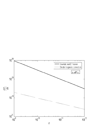
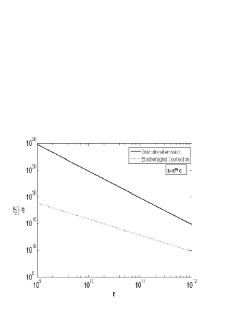
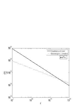
5 Conclusions

GWs science has entered a new era and the recent years have been characterized by several major advances. For what concerns the most promising GW sources for ground-based and space-based detectors, notably, binary systems composed of NS and BHs, our understanding of the two-body problem and the GW generation problem has improved significantly. The best-developed analytic approximation in General Relativity is undoubtable the post-Newtonian method. In this paper, we have calculated the electromagnetic corrections to the GWs emitted by a coalescing binary system. We have considered an electromagnetic dipole-type field and calculated the electromagnetic contribution to the stress-energy tensor. We have obtained a correction to the standard gravitational energy-loss which becomes null setting the magnetic field to zero. In general, the electromagnetic correction term is negligible with respect to the gravitational one. This result holds also for black hole and white dwarfs binary systems. However, there could be coalescing binary systems with a large dipole magnetic momentum and a large orbital radius where the electromagnetic correction to GWs emission is relevant. In particular, the electromagnetic energy emitted by these binary systems is comparable to the gravitational wave output for given values of the magnetic field and of the orbital radius. Revealing such a phenomenon by observations could be an electromagnetic signature for the gravitational waves emission.

References

- Abbott (2010) Abbott B. et al. (LIGO Scientific Collaboration), Class. Quant. Grav. 27, 173001 (2010).
- Anderson et al. (2008) Anderson M., Hirschmann E.W., Lehner L., Liebling S.L., Motl P.M., Neilsen D., Palenzuela C. , Tohline J.E., Phys. Rev. Lett.100, 191101 (2008).
- Apostolatos et al. (1994) Apostolatos T. A., Cutler C., Sussman G. J., Thorne K. S., Phys. Rev. D49, 6274 (1994).
- Apostolatos et al. (1995) Apostolatos T. A., Phys. Rev. D52, 605 (1995).
- Apostolatos et al. (1996) Apostolatos T. A., Phys. Rev. D54, 2438 (1996).
- Arun et al. (2009) Arun K. G., Buonanno A., Faye G., Ochsner E., Phys. Rev. D79, 104023 (2009).
- Arun et al. (2009) Arun K. G., Babak S., Berti E., Cornish N., Cutler C., Gair J., Hughes S. A., Iyer B. R., Lang R. N., Mandel I., Porter E. K., Sathyaprakash B. S., Sinha S., Sintes A. M., Trias M., Van Den Broeck C., Volonteri M., Class. Quantum Grav. 26, 094027 (2009).
- Baiotti et al. (2010) Baiotti L., Damour T., Giacomazzo B., Nagar A., Rezzolla L., arXiv:1009.0521v1 [gr-qc], (2010).
- Barker O’Connell (1975) Barker B. M., O’Connell R. F. , Phys. Rev. D12, 329 (1975).
- Belczynski et al. (2002) Belczynski K., Kalogera V., Bulik T., Astrophys. J., 572, 407 (2002).
- Belczynski et al. (2008) Belczynski K., O’Shaughnessy R., Kalogera V., Rasio F., Taam R. E., Bulik T., Astrophys. J., 680, L129 (2008).
- Berti et al. (2009) Berti E. , Cardoso V., Starinets A. O., Class. Quantum Grav. 26, 163001 (2009).
- Blanchet (2006) Blanchet L., Living Rev. Rel. 9, 4 (2006).
- Blandford Znajek (1977) Blandford R. D., Znajek R. L., Mon. Not. R. Astron. Soc.179, 433 (1977).
- Buonanno Damour (2006) Buonanno A., Chen Y., Damour T., Phys. Rev. D74, 104005 (2006).
- Buonanno Damour (1999) Buonanno A., Damour T., Phys. Rev. D59, 084006 (1999).
- Buonanno Damour (2000) Buonanno A., Damour T., Binary black holes coalescence: transition from adiabatic inspiral to plunge, gr-qc/0011052 (2000).
- Buonanno et al. (2003) Buonanno A., Chen Y., Vallisneri M., Phys. Rev. D67, 104025 (2003).
- Buonanno (2007) Buonanno A., arXiv: 0709.4682v1(2007).
- Capozziello et al. (2010) Capozziello S., De Laurentis M., De Martino I., Formisano M., Astr. Part. Phys. 33, 190, (2010).
- Capozziello et al. (2011) Capozziello S., De Laurentis M., De Martino I., Formisano M., ArXiv:1004.4818 (2010) to appear in Astroph. Sp. Science.
- Chatterji et al. (2005) Chatterji S. et al., Phys. Rev. D74, 082005 (2006).
- Cornish Shapiro Key (2010) Cornish N. J., Shapiro Key J., Phys. Rev. D82 044028 (2010).
- Cutler et al. (1993) Cutler C. et al., Phys. Rev. Lett.70, 2984 (1993).
- Cutler et al. (2005) Cutler C., Gholami I., Krishnan B., Phys. Rev. D72, 042004 (2005).
- Damour et al. (1998) Damour T., Iyer B.R., Sathyaprakash B.S., Phys. Rev. D57: 885 (1998).
- Damour et al. (2000) Damour T., Jaranowski P., Sch fer G., Phys. Rev. D62, 084011 (2000).
- Damour (2001) Damour T., Phys. Rev. D64, 124013 (2001).
- Damour et al. (2002) Damour T., Iyer B., Sathyaprakash B., Phys. Rev. D66, 027502 (2002).
- Damour et al. (2003) Damour T., Iyer B., Sathyaprakash B., Phys. Rev. D67, 064028 (2003).
- di Serafino et al. (2010) di Serafino D., Gomez S., Milano L., Riccio F., Toraldo G., Journal of Global Optimization 48, 41 (2010).
- di Serafino Riccio (2010) di Serafino D., Riccio F., Proceedings of the 18th Euromicro International Conference on Parallel Distributed and Network-Based Processing, 231, (2010).
- Douglas Swesty et al. (2000) Douglas Swesty F. et al., Astrophys. J.541, 937 (2000).
- Duncan Thompson (1992) Duncan R. C. and Thompson C., Astrophys. J., 392, L9 (1992).
- Finn (1992) Finn L.S., Phys. Rev. D46, 5236 (1992).
- Finn Chernoff (1993) Finn L. S. and Chernoff D.F., Phys. Rev. D47, 2198 (1993).
- Flanagan Hughes (1993) Flanagan E.E. and Hughes S.A., Phys. Rev. D 57, 4535 (1998).
- Hulse Taylor (1975) Hulse R. A., Taylor J. H., Astrophys. J., 195, L51 (1975).
- Ioka Taniguchi (2000) Ioka K. and Taniguchi T. , Astrophys. J.537, 327 (2000).
- Kidder et al. (1993) Kidder L. E., Will C. M.,Wiseman A. G. , Phys. Rev. D, 47, R4183 (1993).
- Kidder et al. (1995) Kidder L. E., Phys. Rev. D, 52, 821 (1995).
- Klein Jetzer (2010) Klein A., Jetzer Ph., Phys. Rev. D81, 124001 (2010).
- Kouveliotou et al. (1998) Kouveliotou C. et al., Nature, 393, 235 (1998).
- Lang Hughes (2009) Lang R. N., Hughes S. A., Class. Quantum Grav. 26, 094035 (2009).
- LIGO Collaboration (2009) LIGO Collaboration, Phys. Rev. D80, 047101 (2009);
- Maggiore (2007) Maggiore M., Gravitational Waves: Theory and Experiments, Oxford University Press, USA (2007).
- Macdonald Thorne (1982) Macdonald D. A., Thorne K. S., Mon. Not. R. Astron. Soc.198, 345 (1982).
- Majar Vasth (2008) Maj r J., Vasth M., Phys. Rev. D77, 104005 (2008).
- Majar (2009) Maj r J., Phys. Rev. D, 80, 104028 (2009).
- Misner et al. (1973) Misner C.W., Thorne K.S., Wheeler J.A., Gravitation, Freeman, New York (1973).
- Nice (2003) Nice D. J., Thorsett S., ASP Conf. Series 302, 93 (2003).
- O’Connell (2004) O’Connell R. F., Phys. Rev. Lett.93, 081103 (2004).
- Palenzuela et al. (2009) Palenzuela C., Anderson M., Lehner L., Liebling S.L., Neilsen D., Phys. Rev. Lett.103, 081101 (2009).
- Palenzuela et al. (2010) Palenzuela C., Garrett T., Lehner L., Liebling S.L., Phys. Rev. D82, 044045 (2010).
- Pan et al. (2004) Pan Y. , Buonanno A., Chen Y., Vallisneri M., Phys. Rev. D69, 104017 (2004).
- Phinney (1991) Phinney E. S., Astrophys. J.380, L17 (1991).
- Poisson (1998) Poisson E., Phys. Rev. D57, 5287 (1998).
- Racine (2008) Racine J., Phys. Rev. D78, 044021 (2008).
- Rezzolla et al. (2010) Rezzolla L., Baiotti L., Giacomazzo B., Link D., Font J. A., Class. Quant. Grav. 27, 114105 (2010).
- Rezzolla et al. (2003) ]Rezzolla L, Yoshida S, Maccarone T J and Zanotti O., Mon. Not. R. Astron. Soc.textbf344, L37 (2003).
- Rieth (1997) Rieth R., Sch fer G., Class. Quantum Grav. 14, 2357 (1997).
- Ryan (1996) Ryan F. D.,Phys. Rev. D53, 3064 (1996).
- Sengupta (2009) Sengupta Anand S. for the LIGO Scientific Collaboration and the Virgo Collaboration, LIGO-Virgo searches for gravitational waves from coalescing binaries: a status update, arXiv:0911.2738.
- Shapiro Teukolsky (1983) Shapiro S.L. and Teukolsky S.A., Black Holes, White dwarfs and Neutron Stars. Chicago Univ. Press (Chicago) (1983).
- Sinha Mukhopadhyay (2010) Sinha M. and Mukhopadhyay B., Instability of neutron star matter in high magnetic field: constraint on central magnetic field of magnetars, arXiv:1005.4995(2010).
- Stairs (2004) Stairs I. H., Science 304, 547 (2004).
- Tartaglia Ruggiero (2002) Tartaglia A. and Ruggiero M. L., Nuovo Cim., 117 B, 743-768 (2002).
- Taylor (1989) Taylor G., Astrophys. J.345, 434 (1989).
- Thompson Duncan (1995) Thompson C. and Duncan R. C., Mon. Not. R. Astron. Soc., 275, 255, (1995).
- Usov (1992) Usov V. V., Nature, 357, 472 (1992).
- Vasisht Gotthelf (1997) Vasisht G. and Gotthelf E. F., Astrophys. J., 486, L129 (1997).
- Wang Will (2007) Wang H., Will C. M., Phys. Rev. D, 75, 064017 (2007).
- Weinberg (1972) Weinberg S., Gravitation and Cosmology (New York:Wiley) (1972).
- Weisberg Taylor (2003) Weisberg J. M., Taylor J. H., in Radio Pulsars, ed. M. Bailes.
- Will (2005) Will C. M., Phys. Rev. D71, 084027 (2005).
- Woods et al. (1999) Woods P. M. et al., Astrophys. J., 519, L139 (1999).
- Zeng Will (2007) Zeng J., Will C. M., Gen. Rel. Grav. 39 1661-1673 (2007).
- Znajek (1997) Znajek R. L., Mon. Not. R. Astron. Soc., 179, 457 (1977).