Formation of Gyrs old black holes in the centers of galaxies within the Lemaître–Tolman model

Abstract

In this article we present a model of formation of a galaxy with a black hole in the center. It is based on the Lemaître–Tolman solution and is a refinement of an earlier model. The most important improvement is the choice of the interior geometry of the black hole allowing for the formation of Gyrs old black holes. Other refinements are the use of an arbitrary Friedmann model as the background (unperturbed) initial state and the adaptation of the model to an arbitrary density profile of the galaxy. Our main interest was the M87 galaxy (NGC 4486), which hosts a supermassive black hole of mass $3.2\cdot 10^{9}M_{\odot}$. It is shown that for this particular galaxy, within the framework of our model and for the initial state being a perturbation of the $\Lambda$CDM model, the age of the black hole can be up to $12.7$ Gyrs. The dependence of the model on the chosen parameters at the time of last scattering was also studied. The maximal age of the black hole as a function of the $\Omega_{m}$ and $\Omega_{\Lambda}$ parameters for the M87 galaxy can be $3.717$ or $12.708$ Gyr.

1 Introduction

Recent years brought increasing evidence that large galaxies host massive black holes at their centers. The best evidence was obtained for the Milky Way, due to the proximity of the galactic center located at the distance $R_{0}=8.33\pm 0.35$ kpc. Analysis of orbits of the S-stars cluster near the galactic core, especially the S2 star, allowed to conclude that a mass of $4.31\pm 0.36\cdot 10^{6}M_{\odot}$ is responsible for the apparent movement of the stars Gillessen:2009a ; Gillessen:2009b ; Gualandris:2010 ; Ghez:2008 . Such mass enclosed in a small volume, of radius less than $0.01$ pc, can only be a black hole. The existence of black holes at the centers of galaxies calls for construction of models describing their creation and growth. This work presents improvements to one of such models Krasinski:2004a .

It is thought that the currently existing structures in the Universe (like galaxies, clusters of galaxies and voids) evolved out of small inhomogeneities that are observed as directional variations ($\Delta T/T\approx 10^{-5}$) of the temperature of the cosmic microwave background (CMB) radiation. The generation of these inhomogeneities is a problem only when one insists on using models of the Universe that are born spatially homogeneous. In an inhomogeneous model, such as the Lemaître–Tolman (LT) model used here, the Universe emerges from the Big Bang being already inhomogeneous. The inhomogeneities are generated within the Big Bang and their amplitudes are arbitrary parameters that can be adapted to observational constraints. (But it must be stressed that the LT model, in which the matter is assumed to be dust, cannot be applied to epochs earlier than last scattering. A still more general inhomogeneous model that includes pressure gradients must be used for the pre-last-scattering epoch.) It has already been proven in an earlier paper Krasinski:2004a , using an LT model, that with a suitable choice of the velocity profile at last scattering, an object can be created that has the same density profile at present as the M87 galaxy, and contains a black hole around the center that has the same mass as the black hole in M87. (For an exposition of the method used in Ref. Krasinski:2004a see Refs. Krasinski:2001 ; Krasinski:2004b and Plebanski:2006 .) The black hole is created because matter around the center expands more slowly than farther away, what leads, at a certain moment, to the creation of the apparent horizon surrounding a trapped region, and soon after to the creation of a Big Crunch singularity at the center.

In Ref. Krasinski:2004a two particular configurations of the LT model were considered. In one, the black hole formed around a pre-existing wormhole within a fraction of a second after the Big Bang. In the other, there was no wormhole or black hole initially, and it formed during the evolution of the proto-galaxy. The first configuration is somewhat exotic and we will not pursue it here. The problem with the second configuration was that the implied age of the black hole was only $4\times 10^{8}$ years, what is inconsistent with astrophysical implications 2008MNRAS.391..481S ; 2006ApJ…643..641H ; 2004ApJ…614L..25Y . The reason for the implied definite age was that the LT model used there contained too few free parameters.

This paper is an improvement over Ref. Krasinski:2004a . The method of constructing the model is the same as before. We define a certain density or velocity profile at last scattering, taking care that the amplitude remains within the limits implied by the measurements of the temperature distribution of the CMB radiation. We define another density profile at the present time that agrees with the observationally determined density profile of the M87 galaxy Fabricant:1980 and contains a black hole at the center, of mass $3.2\pm 0.9\cdot 10^{9}M_{\odot}$, equal to the mass of the black hole observed in M87 Macchetto:1997 . The improvement consists in the LT model having more free parameters. Thanks to this, the age of the black hole is no longer determined and can be up to $\sim 12.7$ Gyr, in agreement with what astrophysics tells us 2008MNRAS.391..481S ; 2006ApJ…643..641H ; 2004ApJ…614L..25Y .

Our model has certain weaknesses, of which we are aware, but, just as was stated in Ref. Krasinski:2004a , we treat it as an exploratory step into a new territory: we intend to test a new method that we hope will be improved in the future. The deficiencies to be removed in the future are the following:

1. No real galaxy is spherically symmetric. The model can be said to apply approximately to elliptic galaxies (M87 is one), but spherical symmetry leads to the next problem listed below.

2. Real galaxies rotate. In a spherically symmetric model rotation is necessarily zero. The presence of rotation influences the time scale of evolution, for example, by slowing down the collapse it may significantly delay the formation of the black hole. However, no exact solutions of Einstein’s equations are known that would describe matter that is expanding and rotating at the same time. All known expanding solutions have zero rotation, all known rotating solutions are either stationary or unrealistic for other reasons (for more on this see Ref. Plebanski:2006 ). So if one wishes to have an evolving configuration that can be described by the exact formalism of general relativity, not much is left beyond spherically symmetric models.

3. As was stated in Ref. Krasinski:2004a , the perturbation that would evolve into a single galaxy would have the diameter of approx. 0.004^∘ in the CMB sky. The current best angular resolution of measurements of the temperature fluctuations of the CMB radiation is 0.2^∘ WMAP7:2011a ; WMAP7:2011b . Consequently, the amplitude of fluctuation at this large angular scale does not give us information that we need to constrain our model. Lacking any better possibility, just as in the earlier paper Krasinski:2004a , we took care that the amplitudes of our initial density and velocity profiles do not exceed the limits set at 0.2^∘.

The remarks above show that our toy model cannot be literally taken as the actual model of an existing galaxy. However, it avoids a few other deficiencies that could be contemplated:

1. Once the black hole is formed in an LT model, where pressure is zero and all motions are radial, it keeps accreting matter until it swallows up the whole mass contained in the region where $E<0$. This happens in a finite time, which is arbitrarily long in the neighbourhood of $E=0$. However, if the function $E(M)$ has such a profile that at a certain $M=M_{g}$ $E(M_{g})=0$ and $E(M)>0$ for $M>M_{g}$, then the mass from the region $M\geq M_{g}$ is not accreted onto the galaxy. Thus, $M_{g}$, which is independent of time, can be interpreted as the mass of the galaxy. This is outside the region considered in our paper. The geometrical radius of the $M=M_{g}$ surface will be expanding as dictated by the $E=0$ evolution equation of the LT model. For the surface of a galaxy of radius 32 kpc $\approx 10^{21}$ m and mass $2.4\times 10^{12}M_{\odot}=4.8\times 10^{42}$ kg, if it were to evolve by the $E=0$ Lemaître – Tolman equation ${R,_{t}}^{2}=2M/R$, the current velocity of expansion would be approx. 800 km/s $\approx 8.2\times 10^{-4}$ pc/yr, and constantly decreasing because $\Lambda=0$. This is negligible compared to the error in determining the edge of a galaxy.

2. Each real galaxy is surrounded by vacuum. The cosmological model takes over at a considerably larger scale. If one wants to illustrate this situation in a toy model like ours, it is enough to match our LT galaxy model to the Schwarzschild spacetime at a certain mass $M=M_{g}$, and then to match the Schwarzschild region on the outside to another LT or Friedmann region modelling the Universe. Both matchings would take place outside the region we consider and would have no influence on what happens inside the galaxy. An explicit example of such matchings is given in Ref. Matravers:2001 .

The structure of this paper is as follows. Sec. 2 presents the basic properties of the Lemaître–Tolman model. Sec. 3 briefly outlines the method introduced in Refs. Krasinski:2001 ; Krasinski:2004b and emphasises the key elements of the model. In Sec. 4 we describe the improvements to the basic model: the more general forms of the free functions in the LT model and the more general (and more realistic) density profile of the galaxy at the present time. This section also gives the necessary equations for the use of an arbitrary FLRW model as the background at the initial instant (in Ref. Krasinski:2004a the background was assumed to be spatially flat). Sec. 5 presents the results of application of the model to the M87 galaxy. Evolution from spatially homogeneous initial profiles of velocity and density to a galaxy with a black hole is described. A spatially homogeneous (flat) density profile is obviously within the observational limits on density perturbations, but may lead to the following problem. After the LT model is uniquely determined by the initial and final density profiles, the initial velocity profile that caused the condensation can be calculated from the model and may turn out to have a too large amplitude. The same may happen with the initial velocity profile being flat – the calculated amplitude of the initial density profile may turn out to be too large. Graphs shown in Sec. 5 prove that this did not happen; all implied profiles are consistent with the observational constraints. Sec. 5 also shows how the age of the black hole and the arbitrary functions in the LT model change with the initial FLRW model. The last section contains summary and conclusions.

2 The Lemaître–Tolman model - basic properties

The Lemaître–Tolman model is a spherically symmetric nonstatic solution of the Einstein equations with a dust source Lemaitre:1933.1997 ; Tolman:1934.1997 ; Bondi:1947 . Its metric is

$${\rm d}s^{2}={\rm d}t^{2}-\frac{{R,_{r}}^{2}}{1+2E(r)}{\rm d}r^{2}-R^{2}(t,r)({\rm d}\theta^{2}+\sin^{2}\theta{\rm d}\varphi^{2}),$$ (1)

where $E(r)$ is an arbitrary function arising as an integration constant from the Einstein equations, $R(t,r)$ is a function satisfying

$${R,_{t}}^{2}=2E+2\frac{M}{R}+\frac{1}{3}\Lambda R^{2},$$ (2)

where $\Lambda$ is the cosmological constant and $M(r)$ is another arbitrary function. Equation (2), called the evolution equation, is a first integral of the Einstein equations, $R(t,r)$ is called the areal radius and $R,_{t}$ is referred to as the velocity. The matter density $\rho(t,r)$ is

$$\frac{8\pi G}{c^{4}}\rho=\frac{2M,_{r}}{R^{2}R,_{r}}.$$ (3)

When $\Lambda=0$, equation (2) has three families of solutions depending on the sign of $E(r)$. They are as follows:
$E<0$ – elliptic evolution

$$R(t,r) =\frac{M}{-2E}(1-\cos\eta),$$ (4)

$$\eta-\sin\eta =\frac{(-2E)^{3/2}}{M}(t-t_{B}(r)),$$

$E=0$ – parabolic evolution

$$R(t,r)=\left(\frac{9}{2}M(t-t_{B}(r))^{2}\right)^{1/3},$$ (5)

$E>0$ - hyperbolic evolution

$$R(t,r) =\frac{M}{2E}(\cosh\eta-1),$$ (6)

$$\sinh\eta-\eta =\frac{(2E)^{3/2}}{M}(t-t_{B}(r)),$$

where $\eta$ is a parameter and $t_{B}(r)$ is one more arbitrary integration function called the bang time. The formulas given above are covariant under arbitrary coordinate transformations of the form $r^{\prime}=g(r)$, which allows for $r$ to be chosen freely, what in turn means that one of the three functions $E(r)$, $t_{B}(r)$ and $M(r)$ can be fixed at our convenience by the appropriate choice of $g$.

From the form of the solution in the elliptic case, Eqs. (4), we can deduce that $R(t,r)$ reaches a maximum for each $r$ and then decreases to zero. The values of $\eta$ for which $R(t,r)$ vanishes are $\eta=0$, corresponding to the Big Bang, and $\eta=2\pi$ corresponding to the Big Crunch at $t=t_{C}$

$$t_{C}(r)=t_{B}(r)+\frac{2\pi M}{(-2E)^{3/2}}.$$ (7)

The function $t_{C}(r)$ is called the crunch time function.

The Friedman–Lemaître–Robertson–Walker (FLRW) models arise from the LT models in the limit

$$t_{B}={\rm const},\qquad E=-\frac{1}{2}kr^{2},\qquad M=M_{0}r^{3},$$ (8)

where $k$ and $M_{0}$ are constants.

2.1 Shell crossings

It is important to avoid shell crossings, that is loci of $R,_{r}=0$ and $M,_{r}\neq 0$, where a constant $r$ shell collides with its neighbour (as a consequence of $g_{rr}=0$). Shell crossings are curvature singularities and cause the density to diverge ($\rho\rightarrow\infty$) and change sign to become negative. Such an undesirable behavior can be avoided if the shapes of the three arbitrary functions defining the LT model are chosen appropriately. The general conditions for avoidance of shell crossings are given in Hellaby:1985 ; Hellaby:1986 .

2.2 $M(r)$ as radial coordinate

It is convenient to use $M(r)$ as the radial coordinate, that is $r^{\prime}=M(r)$. It is possible because $M(r)$ will be a strictly growing function, $M,_{r}>0$, in the whole region under consideration. Then we have $R=R(t,M)$, $\rho=\rho(t,M)$ and Eq. (3) becomes

$$\frac{8\pi G}{c^{4}}\rho=\frac{2}{R^{2}R,_{M}}=\frac{6}{(R^{3}),_{M}},$$ (9)

from which we find

$$R^{3}(t,M)-R_{i}^{3}=\frac{3}{4\pi}\int_{M_{i}}^{M}\frac{{\rm d}\xi}{\rho(\xi)},$$ (10)

where $\rho$ is the density profile of the galaxy as a function of $M$, $R_{i}$ and $M_{i}$ are constants to be determined later (see Sec. 4.3). Hereafter we use $M$ as the radial coordinate.

3 A galaxy with a central black hole in the LT model

An LT model is generally specified by defining the shapes of the arbitrary functions $E(M)$ and $t_{B}(M)$, what then allows for the reconstruction of the evolution of the model by using Eqs. (4)–(6). However, it is possible to follow a different path, that is to calculate these functions for a specific density or velocity profiles at any two time instants, as described in Krasinski:2001 and Krasinski:2004b . Moreover, there are no limitations on those profiles (except the obvious one of spherical symmetry). The class of the LT evolution applying to each $M$ value can generally be different, however for the creation of a black hole an LT model must necessarily be recollapsing in the region near the center of symmetry $M=0$.

The main idea of the model constructed in Krasinski:2004a is that a spherically symmetric galaxy with a central black hole can be created from accretion of matter onto an initial fluctuation at recombination. This is the most probable scenario of structure formation in our Universe 2003ApJ…582..559V ; 2002MNRAS.331…98V ; 2003ApJ…596…47S ; 2003ApJ…591..499A ; 2003ApJ…597…21A ; 2008MNRAS.384….2G . Accretion in the model is achieved by a slower expansion near the center, and a faster one further away. We will now briefly describe the main properties of the previously developed model.

3.1 The basic framework of the model

The basic framework of the model was discussed in Krasinski:2004a . The model allows for the formation of a galaxy with a central black hole by accretion of background matter onto an initial fluctuation of density or velocity distribution at the time of last scattering of the CMB. The background is assumed to be Friedmannian (see Sec. 4.3). The input data provided for the model are the profiles of the velocity or the density at last scattering and the current density distribution in the galaxy. In Krasinski:2004a the model was used to create a black hole from a flat (Friedmannian) velocity distribution at last scattering. In this case, the fluctuation was due to the corresponding non–flat density profile. The existence of a black hole at the center of a galaxy is assumed on observational grounds. The mass of the black hole is an input parameter and likewise must be taken from observations. The observational density profile of the galaxy was approximated by a simple function, which allowed for exact calculations.

The construction of the model consisted of the following steps:

1. determining the functions $E(M)$ and $t_{B}(M)$ in the part outside the black hole, that is for the mass range $M>M_{\rm BH}$, where $M_{\rm BH}$ is the observationally determined mass of the black hole in the galaxy,

2. smooth joining of the functions $E(M)$ and $t_{B}(M)$ in the parts inside and outside the black hole i.e. at the boundary $M=M_{\rm BH}$. The part inside the black hole is arbitrary and was assumed to be a simple $E<0$ recollapsing model defined by a choice of the bang and crunch time functions,

3. evolution reconstruction - using the full $E(M)$ and $t_{B}(M)$ functions the evolution of $R(t,M)$ and $\rho(t,M)$ was reconstructed using Eqs. (4)–(6).

In the model the time of the black hole formation is the value of the future apparent horizon at its minimum i.e. $(t_{\rm AH+})_{\rm min}$. However, in this model the crunch time function and the future apparent horizon almost coincide, the instant of the creation of the black hole is very close to $t_{C}(0)$ (see Fig. 4 and Krasinski:2004a for details). The first application of the model was to the M87 galaxy which hosts a supermassive black hole of mass $3.2\cdot 10^{9}M_{\odot}$ Macchetto:1997 , with density profile being an approximation of Fabricant et. al. Fabricant:1980 . In the first parametrization of the black hole’s interior geometry the value of $(t_{\rm AH+})_{\rm min}$ was high, leading to a black hole of the age of a few hundred million years, which is in disagreement with other estimations of supermassive black hole’s age based on the $\Lambda$CDM model 2008MNRAS.391..481S ; 2006ApJ…643..641H ; 2004ApJ…614L..25Y .

4 Development of the model

The model allows for modifications which can lead to more realistic predictions. Particular attention was paid to arrive at such bang and crunch time functions that would give the black hole’s age of the order of Gyr.

4.1 The black hole interior

Name	$t(M)$	$p_{i}$
exp	$p_{1}+p_{2}\exp\left(p_{3}M+p_{4}\right)$	$p_{1}\sim t(M_{\rm BH})$ $p_{2}\sim 10^{0}$
hyp	$p_{1}+p_{2}\cosh\left(p_{3}M+p_{4}\right)$	$p_{3}\sim 10^{2}$ $p_{4}\sim 10^{2}$

Table 1: Parametrizations of the interior bang and crunch time functions. The table shows the bang and crunch time functions inside the black hole. The third column gives a general order of magnitude of the value of each parameter. $t(M_{\rm BH})$ means that the value of the parameter is of the order of the value of the bang or crunch time function at $M=M_{\rm BH}$. For $t_{B}(M)$ the parameters $p_{i}$ are denoted $b_{i}$, and for $t_{C}(M)$ by $c_{i}$.

The first modification concentrates on the functions $t_{B}(M)$ and $t_{C}(M)$ that define the black hole’s interior, for which, for fundamental reasons, no observational data exist. Therefore, we are free to choose any parametrization and the only condition is to join it smoothly to the galaxy model. In the most probable scenarios of black hole creation, it is formed by a collapse of a massive object. We used exponential and hyperbolic functions to parameterize the interior functions $t_{B}(M)$ and $t_{C}(M)$, see Table 1. The chosen forms of the functions have $8$ parameters: $b_{1}$, $b_{2}$, $b_{3}$, $b_{4}$ for $t_{B}(M)$ and $c_{1}$, $c_{2}$, $c_{3}$, $c_{4}$ for $t_{C}(M)$.

A smooth match of the interior and exterior requires the continuity of the functions $E(M)$ and $t_{B}(M)$ and their derivatives at the boundary $M=M_{\rm BH}$ (the Darmois/Lichnerowicz junction conditions), this is also a sufficient condition Bonnor:1981 . Therefore, the following system of equations has to be solved for the parameters $b_{i}$ of $t_{B}(M)$ and $c_{i}$ of $t_{C}(M)$, $i=1,\ldots,4$:

$$t_{B}(M_{\rm BH},b_{1},b_{2},b_{3},b_{4}) =\left[t_{B}\right]_{M=M_{\rm BH}},$$ (11)

$$\frac{{\rm d}{t_{B}}}{{\rm d}{M}}\Bigl{(}M_{\rm BH},b_{1},b_{2},b_{3},b_{4}\Bigr{)} =\left[\frac{{\rm d}{t_{B}}}{{\rm d}{M}}\right]_{M=M_{\rm BH}},$$

$$E(M_{\rm BH},b_{1},b_{2},b_{3},b_{4},$$

$$c_{1},c_{2},c_{3},c_{4}) =\left[E\right]_{M=M_{\rm BH}},$$

$$\frac{{\rm d}{E}}{{\rm d}{M}}\Bigl{(}M_{\rm BH},b_{1},b_{2},b_{3},b_{4},$$

$$c_{1},c_{2},c_{3},c_{4}\Bigr{)} =\left[\frac{{\rm d}{E}}{{\rm d}{M}}\right]_{M=M_{\rm BH}},$$

where the expressions on the left hand side are the analytical functions depending on the chosen parametrization and the expressions on the right hand side are the numerically found values of $t_{B}(M)$ and $E(M)$ for $M=M_{\rm BH}$, using the method described in Krasinski:2004a . The analytical expression for $E(M)$ is based on Eq. (7). However, the assumed bang and crunch time functions have eight unknown parameters, whereas from (11) only four parameters can be determined. Therefore, the values of the other four parameters have to be supplied. To accomplish that we choose any two parameters for $t_{B}(M)$ and any two parameters for $t_{C}(M)$, and set their values using random numbers. The difficulty here (from the numerical point of view) is to determine the order of magnitude of the parameters, but this can be achieved by examination of the type of parameterized equation (see column $3$ of Table 1). The system of equations (11) has to be solved numerically. The usage of random numbers does not have any impact on the analysis as the multidimensional minimalization methods, employed further for finding extreme LT models take the random values only as the starting values for subsequent optimalization.

4.2 The density profile of the galaxy

A galaxy in the constructed model is described by a density profile and the mass of the black hole. However, the quantity used in the numerical calculations is the areal radius $R(t_{0},M)$ corresponding to that (spherically symmetric) density profile, where $t_{0}$ is the present age of the Universe. The equation used for finding its value is (10), with $\rho$ being a function of $M$. Therefore, the general $r$ coordinate representing the distance from the center of symmetry must be replaced by the mass $M$ of the sphere of radius $r$. In Krasinski:2004a the relation $r=r(M)$ was found analytically, using an analytically convenient approximation to the observational density profile of the galaxy. However, we would like to apply the model to any galaxy with known density profile which is suspected of hosting a black hole of known mass. In such a general situation, galaxies are described by density profiles which do not allow for analytical calculation of the relation $r=r(M)$. Therefore, we must resort to numerical calculations and take $\rho(M)\ {\overset{\rm def}{=}}\ \rho(r(M))$, where $r(M)$ is the inverse function to $M(r)$ and is found numerically.

In order to find the areal radius $R(t_{0},M)$, the constants $M_{i}$ and $R_{i}$ of Eq. (10) have to be appropriately chosen. We may put $R_{i}=0$, thus assuming $R(t_{0},M_{i})=0$. Further we specify $M_{i}$ to be $M_{S}$ – the mass already swallowed by the singularity. On a spacetime diagram in the coordinates $(M,t)$ that mass is represented by the value of $M$, for which the line $t=t_{0}$, representing the present moment, intersects the crunch time function, that is $t_{0}=t_{C}(M_{S})$ (see Fig. 4). Therefore Eq. (10) becomes

$$R^{3}\left(t_{0},M\right)=\frac{3}{4\pi}\int_{M_{S}}^{M}\frac{{\rm d}\xi}{\rho\left(\xi\right)}.$$ (12)

The value of $M_{S}$ can be calculated using the properties of the apparent horizon (see Krasinski:2004a , Plebanski:2006 ). Only for $\rho(M)$ given in a fairly simple form analytical calculations are possible. Here, we do not find the value of $M_{S}$ and make use of the properties of the apparent horizon.

The apparent horizon consists of the events for which

$$R(M_{\rm BH})=2M_{\rm BH},$$ (13)

where $M_{\rm BH}$ is the mass of the black hole Plebanski:2006 ; Szekeres:1975 . We also have $M_{S}<M_{\rm BH}$, that is the mass swallowed up by the singularity must necessarily be smaller than the mass of the black hole. Therefore we have

$$R^{3}(t_{0},M)=\frac{3}{4\pi}\int_{M_{S}}^{M_{\rm BH}}\frac{{\rm d}\xi}{\rho\left(\xi\right)}+\frac{3}{4\pi}\int_{M_{\rm BH}}^{M}\frac{{\rm d}\xi}{\rho\left(\xi\right)}.$$ (14)

The first term, from the definition of the apparent horizon, is equal to $(2M_{\rm BH})^{3}$ and the equation for calculating the value of areal radius for the galaxy under consideration becomes

$$R(t_{0},M)=\left[(2M_{\rm BH})^{3}+\frac{3}{4\pi}\int_{M_{\rm BH}}^{M}\frac{{\rm d}\xi}{\rho\left(\xi\right)}\right]^{1/3}.$$ (15)

The advantage of this equation is that it can be applied to any galaxy with known density profile and known mass of the black hole.

4.3 The parameters at the recombination

Figure 1: 1 The time of last scattering of CMB in the FLRW model as a function of $\Omega_{\Lambda}$ for different values of $\Omega_{0}$. For the $\Lambda$CDM model with WMAP 7-year results the instant of last scattering is at $t_{\rm rec}=494$ kyr, which is marked with a cross in the plot. 1 The age of the Universe for the same set of $\Omega_{\Lambda}$ and $\Omega_{0}$ values. The cross at $t_{\rm now}=13.727$ Gyr indicates the age of the Universe for the $\Lambda$CDM model with WMAP 7-year results. 1 $a=R/M^{1/3}$ and 1 $b=R,_{t}/M^{1/3}$ at the time of last scattering of CMB in the FLRW model for the same set of $\Omega_{\Lambda}$ and $\Omega_{0}$ values. For the $\Lambda$CDM model with WMAP 7-year results $a$ equals $1.649\cdot 10^{5}$ m^-1/3, while $b$ is equal to $3.483\cdot 10^{-3}$ m^-1/3.

In Krasinski:2004a the parameters at the time of last scattering where chosen to match those of the $k=0$ FLRW model. In this work we will use general FLRW models with $k\neq 0$ and with nonvanishing cosmological constant. The areal radius $R(t,M)$ and the scale factor $S(t)$ of the FLRW model are connected by

$$R(t,M)=r(M)\,S(t),$$ (16)

with $M$ as the radial coordinate. Using the limiting conditions for the FLRW model arising from the LT model, i.e. Eq. (8), we have

$$R(t,M)=M_{0}^{-1/3}M^{1/3}S(t),$$ (17)

where the constant $M_{0}$ determines the particular FLRW model. The value of this constant can be found by comparison of the solutions of the LT model (Eqs. (4)–(6)) with the solutions of the FLRW model Plebanski:2006 , obtaining

$$M_{0}=\frac{4}{3}\frac{G}{c^{2}}\pi\rho(t)S^{3}(t),$$ (18)

where $\rho(t)$ is the (homogeneous) density. By taking the values of $\rho(t)$ and $S(t)$ at the present moment $t=t_{0}$, that is

$$\rho(t_{0})=\Omega_{m}\,\rho_{\rm crit}=\Omega_{m}\,\frac{3H_{0}^{2}}{8\pi G},\qquad S(t_{0})=1,$$ (19)

where $\Omega_{m}$ is the density parameter of matter (with equation of state $p=0$), $\rho_{\rm crit}$ is the critical density with the current estimate of the Hubble constant $H_{0}=71\pm 2.5$ km s^-1 Mpc^-1, based on the latest WMAP results WMAP7:2011a , we get the value for $M_{0}$ as

$$M_{0}=\frac{1}{2c^{2}}\Omega_{m}H_{0}^{2}.$$ (20)

The value of the scale factor $S(t)$ at the time of recombination (last scattering of CMB) is found from

$$S(t_{\rm rec})=\frac{S(t_{0})}{1+z_{\rm rec}}=\frac{1}{1+z_{\rm rec}},$$ (21)

where $z_{\rm rec}=1088.2\pm 1.2$ is the redshift of CMB from the WMAP results. The derivative of the scale factor is determined by the Friedmann equation

$$\left(\frac{{S,_{t}}}{S}\right)^{2}=\frac{8\pi G}{3}\rho_{m}-\frac{k}{S^{2}}+\Lambda,$$ (22)

with the constant $k$ given by

$$k=H_{0}^{2}S^{2}(t_{0})(\Omega_{m}+\Omega_{\Lambda}-1)=H_{0}^{2}(\Omega_{0}-1),$$ (23)

where $\Omega_{\Lambda}=(3/8\pi G)(\Lambda/\rho_{\rm crit})$ and $\Omega_{0}=\Omega_{m}+\Omega_{\Lambda}$.

We would like to find the dependence of our model on the $\Omega_{m}$ and $\Omega_{\Lambda}$ parameters of the FLRW model used to determine the functions at the time of last scattering. In order to do that we need to know the age of the Universe and the recombination time for FLRW models with different $\Omega_{m}$ and $\Omega_{\Lambda}$. From the Friedmann equation, using the normalization $S(t_{0})=1$, the age of the Universe $t_{0}$ is determined by

$$t_{0}=H_{0}^{-1}\int_{0}^{1}\frac{{\rm d}\xi}{\sqrt{\Omega_{m}/\xi-(\Omega_{m}+\Omega_{\Lambda}-1)+\Omega_{\Lambda}\xi^{2}}}.$$ (24)

The instant of last scattering of CMB, used as one of the input parameters for the model, is dependent on the matter content of the Universe. This instant is defined by such density of the radiation that the energy of the photon becomes smaller than the ionization energy of the hydrogen atom. As the radiation and matter have different equations of state, the instant of last scattering is different for different density parameters. The time of last scattering of CMB can be found from the equation similar to Eq. (24), but with the upper limit in the integral replaced by $S(t_{\rm rec})$, taken from Eq. (21). Figure 1 shows the age of the Universe and the instant of recombination as a function of $\Omega_{\Lambda}$ for different values of $\Omega_{0}$. This figure also shows the dependence of the two functions used as input data for the model $a(M)=R(M)/M^{1/3}$ and $b(M)=R,_{t}(M)/M^{1/3}$ at the recombination on the value of $\Omega_{\Lambda}$ for the same set of $\Omega_{0}$ values. The two parameters are constant within a FLRW model and their values for the $\Lambda$CDM model, in units described in 4.4 and with WMAP 7-year results, are $a=1.649\cdot 10^{5}$ m^-1/3 and $b=3.483\cdot 10^{-3}$ m^-1/3.

4.4 The units

Throughout this article we have used the geometric units where both $c$ and $G$ are equal to unity. In order to avoid large numerical values we used $10^{11}M_{\odot}$ as the unit of mass. This value corresponds roughly to the mass of the M87 galaxy.

5 Application of the model to the M87 galaxy

We have tested the constructed model on the M87 (NGC 4486) galaxy, which hosts a supermassive black hole of mass $3.2\cdot 10^{9}M_{\odot}$ and is about $16$ Mpc away from the Earth Macchetto:1997 . The galaxy is mainly known for its highly relativistic jet, but we are only interested in its density profile and the mass of the supermassive black hole in the center.

5.1 The M87 input parameters

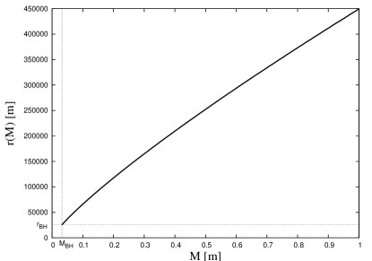
Figure 2: 2 Comparison of M87 density profiles. All curves start at $M=M_{\rm BH}$, which for Fabricant et. al. is equal to $0.03$ m, and $0.032$ m for both Wu, Tremaine profiles. The profile used in our calculation is ’Wu, Tremaine isotropic’. Both axes are in geometric units. 2 The distance–mass relation for the M87 galaxy with the ’Wu, Tremaine isotropic’ density profile. The mass equal to the mass of the black hole is enclosed within the radius $r_{\rm BH}=25538.6$ m. 2 $R(M)$ and 2 $a(M)$ functions for the chosen density profile of Eq. (25). The dotted vertical line represents the black hole’s surface at $M_{\rm BH}=0.032$ m.

In Krasinski:2004a the authors used the approximated profile of Fabricant et. al. Fabricant:1980 , with the mass of the black hole $M_{\rm BH}=0.03$ m. As was described in Sec. 4.2, we no longer have to use any approximation to the density profile and generally we could use the original, not approximated profile, and the value of $M_{\rm BH}$ for our numerical calculations. However, in recent years the standard value of $M_{\rm BH}$ and the shape of the density profile for M87 have changed (see Fig. 2). We will use the updated values.

The M87 galaxy is a radio source, and has been the subject of many measurements based on different methods. In this work we used the ’isotropic’ profile of Wu, Tremaine Wu:2006 based on globular clusters data, given by

$$\rho(r)=\rho_{0}\left(\frac{r}{r_{0}}\right)^{-\alpha},$$ (25)

with the values of the parameters: $r_{0}=19$ kpc, $\rho_{0}=1.9\cdot 10^{7}M_{\odot}$ kpc^-3 and $\alpha=1.8$. The mass of the black hole is assumed to be $3.2\cdot 10^{9}M_{\odot}$. The ’anisotropic’ profile based on the same data, but modified method, differs only in the value of $\alpha$, which for this profile is equal to $1.6$. The three density profiles are plotted in Fig. 2. Note the change in the magnitude of the density values.

The quantities used in our calculations that describe the M87 galaxy, besides $M_{\rm BH}$, are the distance–mass relation $r(M)$, the areal radius $R(t_{0},M)$ and $a(M)=R/M^{1/3}$. The distance–mass relation is found numerically by integration of the density profile and the areal radius $R(t_{0},M)$ is found using Eq. (15). The three functions are plotted in Figs. 2–2.

5.2 The scheme of the method

The general scheme of our method is as follows. Firstly, for the given velocity or density profile at the last scattering and the M87 density profile (together with the assumed $M_{\rm BH}$), the functions $E(M)$ and $t_{B}(M)$ (and also the resulting $t_{C}(M)$) are found in the part outside the black hole, that is for $M>M_{\rm BH}$. Secondly, for the chosen type of black hole interior, that is the bang and crunch time functions for $M<M_{\rm BH}$ described by the equations in Table 1, random four parameters of those equations are chosen and their values are set using uniformly distributed random numbers in the appropriate range, depending on the parameter. Then, the values of the other four parameters are found by numerically solving the equations (11). This is done using multidimensional root finding method based on the Hybrid Method. In this way an LT model model near $M=0$ is found (necessarily recollapsing), which will serve as the starting point for further actions. With some density profiles (at $t={\rm now}$ and at last scattering) it may turn out that the model is not recollapsing at present. This step is necessary to make sure that this does not happen.

As stated before, for galaxies that host supermassive black holes, such as M87, we are mainly interested in finding such an LT model, that would yield a black hole of the age of Gyr. Therefore the age of the black hole is the parameter to be optimized. Optimization is done using the Simplex algorithm of Nelder and Mead for minimization of multidimensional functions Nelder:1965 by again choosing arbitrary four parameters of bang and crunch time functions in the interior of the black hole (found in the previous step) and finding such values of those parameters that would give a black hole of maximal age. For each run we have also found the LT model of minimal age of the black hole, just as a comparison to the maximal one. After this we have performed the reconstruction of evolution together with the calculation of other valuable data.

5.3 The $\Lambda$CDM model of initial fluctuation

Figure 3: 3 The ratio of the density at the recombination $\rho_{\rm rec}(M)$ corresponding to the homogeneous velocity profile of the standard $\Lambda$CDM model to the $\Lambda$CDM density in the same model. The nonuniformness of this profile is responsible for the creation of a galaxy with a central black hole. 3–3 The main panel on both plots shows the $t_{B}(M)$ and $E(M)$ functions for the maximal and minimal age of the black hole. The maximal age is $12.719$ Gyr, the minimal one is $0.428$ Gyr. The functions are calculated for an evolution from a homogeneous velocity profile at the recombination consistent with the $\Lambda$CDM model with $\Omega_{m}=0.266$, $\Omega_{\Lambda}=0.734$. The bang and crunch time functions inside the black hole are parameterized by the hyperbolic function of Table 1. For $M>M_{\rm BH}$ the functions are identical, and dependent only on the input profiles. The difference is inside the black hole ($M<M_{\rm BH}$) and is exhibited in the inset. The ratio of the two functions is plotted in the bottom panel. 3 The main panel shows the $t_{C}(M)$ function for the LT model of maximal and minimal age of the black hole. The optimization parameters are the same as described in 3 and 3. Note the logarithmic scale for the $x$ axis. The $y$ axis is logarithmic up to the value of $t_{C}(M_{\rm BH})=8.7945\cdot 10^{11}\leavevmode\nobreak\ \mathrm{m}\approx t_{0}$, above that value the scale is linear. This is done in order to make the plot readable, as there is a significant difference in the black hole’s creation time, that is the value of $t_{\rm AH+}$ at the minimum, which for the maximal model is equal to $6.458\cdot 10^{10}$ m. The ratio of the two functions is plotted in the bottom panel. The dotted vertical line in all plots represents the boundary of the black hole at $M_{\rm BH}=0.032$ m.

The current concordance cosmological model is the homogeneous $\Lambda$CDM model with $H_{0}=71\pm 2.5$ km s^-1 Mpc^-1, $\Omega_{m}=0.266$ and $\Omega_{\Lambda}=0.734$, based on the latest WMAP results WMAP7:2011a . In our calculation we used the parameters of this model, described by the equations in Sec. 4.3, for the initial state. The constructed model of a galaxy with a black hole takes as the input data for the initial fluctuation at last scattering the profiles of either velocity $R,_{t}(M)$, or density $\rho(M)$. Firstly we will present the results of optimization of black hole’s age for the M87 galaxy evolving from the velocity profile coinciding with that of the $\Lambda$CDM model.

5.3.1 The velocity profile

The quantity that is used in our calculations for this evolution type is $b=R,_{t}(M)/M^{1/3}$. In an FLRW model it depends only on time, and for $\Omega_{m}=0.266$, $\Omega_{\Lambda}=0.734$ its value at recombination is equal to $3.483\cdot 10^{-3}$ m^-1/3. The homogeneity of the chosen velocity profile does not prevent the creation of a galaxy as the corresponding profile of density at last scattering, shown in Fig. 3, is nonuniform, and an initial fluctuation appears and can gain mass through accretion.

Figures 3, 3 and 3 show the main results of optimalization of the age of black hole for the evolution from flat velocity profile at recombination. The bang and crunch time functions were parameterized by the hyperbolic functions of Table 1. The black hole of maximal age is formed at $6.458\cdot 10^{10}$ m, what means that the age of such a black hole is $12.719$ Gyr. The corresponding values for the minimal age are $8.5197\cdot 10^{11}$ m and $0.428$ Gyr. The last number is roughly equal to the value obtained in Krasinski:2004a . Other parameters of the model are summarized in Table 2.

quantity	min	max
BH age [Gyr]	$0.428888$	$12.719398$
$(t_{\rm AH+})_{\rm min}$ [$10^{10}$ m]	$85.197$	$6.458$
$b_{1}$ [$10^{5}$]	$1.156$	$1.160$
$b_{2}$	$374.749$	$-8.460\cdot 10^{-6}$
$b_{3}$	$-0.432$	$64.205$
$b_{4}$	$0.629$	$10.819$
$c_{1}$ [$10^{11}$]	$4.121$	$8.855$
$c_{2}$	$3.628\cdot 10^{11}$	$-3.858\cdot 10^{-19}$
$c_{3}$	$3.163$	$-153.308$
$c_{4}$	$0.641$	$70.526$

Table 2: The parameters of the black hole’s bang and crunch time functions for the models of minimal and maximal age of the black hole. The parameters labeled as $b_{i}$ describe the bang time function, $c_{i}$ describe the crunch time function. The initial conditions correspond to those of Fig. 3.

As we can see in Fig. 3 the value of the crunch time function at $M_{\rm BH}$ is extremely close to $t_{0}$. However, in the model the crunch time is equal to $t_{0}$ not for $M_{\rm BH}$, but for $M_{S}$, the mass swallowed by the singularity, which is necessarily smaller than the mass of the black hole. On the other hand $M_{\rm BH}$ is that value for which the future apparent horizon crosses the present time. Figure 4 shows this situation in an illustrative way, with the bang and crunch time functions chosen so as to make the plot readable.

Figure 4: Evolution leading to a black hole in the $E<0$ LT model. This a copy of Fig. 1 from Krasinski:2004a , where the bang and crunch time functions were chosen so as to make the plot readable and illustrative. Intersections of the line $t={\rm now}$ with the lines representing the Big Crunch and the future apparent horizon AH+ determine the masses $M_{S}$ and $M_{\rm BH}$, respectively. AH– stands for past apparent horizon and ths for time, when the future apparent horizon first appears.

Such behaviour is a consequence of the very small difference between the future apparent horizon and the crunch time function, which causes $M_{S}$ and $M_{\rm BH}$ to almost coincide. The value of $M_{S}$ cannot be found analytically for a general observational density profile of the galaxy. In our calculations we have used the method described in Sec. 4.2 that does not require the knowledge of the value of $M_{S}$.

The maximal age of the black hole obtained here is in good agreement with the estimates based on other models. Figure 5 shows the time and radial dependence of the areal radius $R(t,M)$. As follows from the negative value of $E$, the whole region of spacetime under consideration is recollapsing by now. The flat part of the graph, for which $t>(t_{\rm AH+})_{\rm min}$, is the region of spacetime where the singularity already exists.

In Fig. 5 the constant $M$ slices of $R(t,M)$ for characteristic $M$ values are shown. The first nonvanishing $M={\rm const}$ slice is for a small $M$, chosen arbitrarily to be $10^{-30}$. The whole region under consideration is recollapsing by now, but only the region $M\leqslant M_{\rm BH}$ is within the black hole. Characteristic $t={\rm const}$ slices are plotted in Fig. 5. The upper plot shows the $t={\rm const}$ curve for the instant of recombination, the middle one shows the curves for the time of the creation of the black hole and for the time it was half its present age, the bottom one shows the curve for the present moment. All the curves for $t$ values ranging from the recombination time $t_{\rm rec}$ to the moment of the black hole creation $(t_{\rm AH+})_{\rm min}$ start at the point $M=0$, $R=0$. All the curves for larger $t$ values start at $M\neq 0$, $R=0$, because of the formation and growth of the black hole.

Figure 5: 5 The function $R(t,M)$ for the evolution from flat velocity profile at the recombination. The $M$ axis is in logarithmic units in order to enhance the region near the center of symmetry. Note the inscribed crunch time function in the $R=0$ plane - the crunch time function borders the black hole’s interior. 5 Characteristic $M={\rm const}$ slices of the areal radius. Only those slices for which $M<M_{\rm BH}$ reach the black hole. The $M=1$ slice, corresponding to the region furthermost from the center of symmetry, is recollapsing, but not yet in the final singularity. The $M=M_{\rm BH}$ slice also does not reach the black hole - its value at $t=t_{0}$ is $2M_{\rm BH}$. ’$t_{\rm rec}$’ stands for the time of recombination. 5 Characteristic $t={\rm const}$ slices of the areal radius. The upper plot shows the curve for the instant of recombination, the middle one shows the curves for the time of the creation of the black hole and for the time when it was half its present age, the bottom one shows the curve for the present moment. The curves for times after the creation of the black hole do not start at $M=0$ as the black hole is already created.

5.3.2 The interior parametrization of the black hole

Figure 6: The difference between the hyperbolic and exponential parametrization of the black hole interior. The plots show the ratio of the bang 6 and the crunch 6 time functions subtracted from unity in order to make the values readable. The difference between the functions can be neglected. The shape of the bang time curve for $M>M_{\rm BH}$ is due to the numerical errors, as this $M$ range corresponds to the exterior of the black hole where the type of parametrization of the interior does not affect the values of the functions.

All the results presented so far were found for the bang and crunch time functions of the black hole interior given by the hyperbolic function of Table 1. However, the calculations can be performed for an arbitrary type of the interior of the black hole. Figure 6 presents the comparison between the hyperbolic and the exponential parametrization. The bang and crunch time functions are very similar, their ratio differs from unity by a number of the order of $10^{-8}$ for the bang and $10^{-3}$ for the crunch time function. The maximal age of the black hole is almost the same for the two types of parametrization. Therefore in the following we have chosen only the hyperbolic parametrization of the interior of the black hole functions.

5.3.3 The density profile

An initial fluctuation at the recombination can also be defined by a density profile, that is the function $\rho_{\rm rec}(M)$. The quantity that is used here in calculations is $a=R/M^{1/3}$, where the areal radius at the recombination is found using the modified Eq. (15), without the first term in square brackets and setting the lower limit of the integral to zero. As in the evolution from a given velocity profile at last scattering, we set the density profile to the one corresponding to the $\Lambda$CDM model with $\Omega_{m}=0.266$ and $\Omega_{\Lambda}=0.734$. Then the density profile is flat and the value of $a$ is equal to $1.649\cdot 10^{5}$ m^-1/3.

The corresponding profile of velocity $R,_{t}(M)$ is presented in Fig. 7. This profile exhibits nonuniformness enabling the creation of a black hole. However, the nature of the fluctuation is different than in the case of a flat velocity profile and its corresponding density profile in Fig. 3. In the model the density at the center increases by accretion of background matter, which is achieved by a lower expansion rate near the center and a higher rate further away. The difference in expansion rates is the underlying reason of accretion and the creation of black hole. Therefore, any velocity profile at last scattering that could lead to the creation of a galaxy with a black hole must necessarily be monotonically increasing as a function of $M$. Such a behaviour can be seen in Fig. 7.

The results of our calculations for the evolution form a flat density profile coinciding with the $\Lambda$CDM profile are presented in Figs. 7–7. The $E(M)$ functions are similar in both cases and the whole $M$ range is recollapsing which is necessary for the creation of a black hole. The main difference compared to the previous evolution type is in the bang time function $t_{B}(M)$ which is increasing. This means that the conditions of avoidance of shell crossings are not fulfilled and a shell crossing is imminent. However, due to the values of $t_{B}(M)$ it will occur after the present time and not in the range of application of the model. Figure 8 shows the points where the shell crossings appear. We can see that for the points near the black hole it appears after the present moment. The non–occurrence of the shell crossing in the area covered by the model can also be seen in Fig. 8 where there are no points (besides the black hole interior) where $R,_{M}=0$. The small difference in the LT model functions means that the ages of black holes in both evolution scenarios are the same, within the numerical errors. Other parameters of the bang and crunch time functions are shown in Table 3.

quantity	min	max
BH age [Gyr]	$0.429112$	$12.719378$
$(t_{\rm AH+})_{\rm min}$ [$10^{10}$ m]	$8.5195$	$6.4583$
$b_{1}$ [$10^{4}$]	$-2.890$	$-2.911$
$b_{2}$	$-94.851$	$2.141\cdot 10^{-6}$
$b_{3}$	$-0.432$	$64.205$
$b_{4}$	$0.629$	$10.819$
$c_{1}$ [$10^{11}$]	$4.119$	$8.855$
$c_{2}$	$3.630\cdot 10^{11}$	$-3.858\cdot 10^{-19}$
$c_{3}$	$3.163$	$-153.308$
$c_{4}$	$0.641$	$70.526$

Table 3: The parameters of the bang and crunch time functions of the interior of the black hole for the LT models of minimal and maximal age of the black hole for evolution from a flat density profile coinciding with the standard $\Lambda$CDM model. As before, the parameters labeled as $b_{i}$ describe the bang time function, $c_{i}$ describe the crunch time function.

Figure 7: 7 The ratio of the velocity at last scattering corresponding to a flat density profile, to the $\Lambda$CDM velocity. A monotonic increase of this function enables the creation of a galaxy with a black hole. 7 The bang time function for the evolution from the flat density profile for the maximal and minimal age of the black hole models. The main panel shows the functions for the whole $M$ range, the inset shows the functions near the center of symmetry at $M=0$ and the bottom one shows the ratio of the maximal model to the minimal. Note the difference from the bang time function for the evolution from flat velocity profile in Fig. 3. This function being increasing indicates that there is a shell crossing in the model, but it appears outside the range of the application of the model. 7 The corresponding $E(M)$ function in the same range as for the velocity evolution in Fig. 3. The difference between this and the flat velocity evolution is very small. 7 In the main panel: the crunch time function for the maximal an minimal black hole models. The age of the black hole for the maximal model is $12.719$ Gyr, and $0.429$ Gyr for the minimal one, the same values (within numerical errors) as for the evolution from a flat velocity profile. Note the logarithmic $x$ axis.

Figure 8: 8 The coordinates of the points where the shell crossing singularity occurs. The shell crossing appears after the present moment, i.e. not in the range of application of the model. 8 Evolution of the areal radius $R(t,M)$ for the evolution from a flat density profile at the recombination. There are no shell crossings as there are no points (besides the black hole interior) where $R,_{M}=0$.

5.4 The parameters at the recombination

The results presented so far were obtained for a flat velocity and flat density profiles at the recombination consistent with the $\Lambda$CDM model with $\Omega_{m}=0.266$ and $\Omega_{\Lambda}=0.734$. However, the specific initial FLRW model should not play a key role in the creation of Gyrs old black holes. Therefore, we have performed calculations of the maximal age of the black hole for two types of evolution for initial models with different parameters. We set the Hubble parameter value at $H_{0}=71$ km s^-1 Mpc^-1 and the redshift of the CMB at $z_{\rm rec}=1090$, based on WMPA 7–year results, and carried out the calculations for varying $\Omega_{m}$ and $\Omega_{\Lambda}$ values.

5.4.1 The age of the black hole

In Fig. LABEL:Fig:const_omega_zero_analysis-BH_age the dependence of the maximal age of the black hole on the matter density parameter $\Omega_{m}$, for three constant values of $\Omega_{0}$ equal to $0.5$, $1.0$ and $1.5$, is shown. For both evolution types we can clearly see the two constant values of the maximal age of the black hole equal to $3.717$ and $12.708$ Gyr. For $\Omega_{0}=0.5$ only the first value is obtained. The shapes of the curves for the same value of $\Omega_{0}$ and different evolution types are very similar. The differences are caused by numerical errors and are remnants of the method of choosing initial conditions for the optimization method involving random numbers. These differences are presented in the insets in the $\Omega_{0}=1.5$ plots.

5.4.2 The LT functions

Figure LABEL:Fig:const_omega_zero_analysis-functions shows the $E(M)$ and $t_{C}(M)$ functions for the same three values of $\Omega_{0}$ as in Fig. LABEL:Fig:const_omega_zero_analysis-BH_age for the evolution form flat velocity at the recombination. For the $E(M)$ function all the curves are similar, without any hints of the two values of the age of black holes. The plots for the crunch time function reveal the existence of the two values, as for all values of $\Omega_{0}$ we can indicate the two distinctive families of curves. Because of the fact that the crunch time function and the future apparent horizon $t_{\rm AH+}$ almost coincide in all the cases and taking into account that the value of the future apparent horizon at its minimum is the creation time of the black hole, we can say that the crunch time curves starting at lower values correspond to the higher value of the maximal age of the black hole. The reason why all the crunch time curves corresponding to one value of the age of the black hole, e.g. $12.708$ Gyr, do not start at the same point is that with varying $\Omega_{m}$ the age of the Universe changes.

6 Summary and conclusions

We have demonstrated that within the inhomogeneous LT model a perturbation of the velocity or density profile at the recombination can evolve into a spherically symmetric galaxy–like object with a black hole at the center of the age of Gyr. This work is a refinement to the model presented in Krasinski:2004a , which allows for such an early creation of black holes, together with the usage of an arbitrary density profile describing the present day galaxy and an arbitrary FLRW model as the background matter reservoir. The evolution of such a perturbation leading to the present mass distribution of a galaxy progresses without any shell crossing singularities. In the model, the mass at the center increases in consequence of different expansion rates in the central region and farther away. The crucial point for the time of the black hole creation is the interior geometry of the black hole, that is the bang time function $t_{B}$ and the crunch time function $t_{C}(M)$ in the region $M<M_{\rm BH}$. By an adequate adjustment of those arbitrary functions, we were able to find an LT model yielding the desired age of Gyrs. It was found that the maximal age of the black hole as a function of the density parameters $\Omega_{m}$ and $\Omega_{\Lambda}$ takes a constant value irrespective of the $\Omega_{0}$ value.

The main target for the model was the proper simulation of the black hole at the center of M87 galaxy. This supermassive black hole is one of the biggest supermassive black holes found. We have used a new density profile describing the mass distribution in this galaxy together with an updated value of the mass of the black hole based on Macchetto:1997 . This required a slight improvement of the basic model allowing to use any density profile, not only the one for which analytical calculations are possible. We have successfully obtained an LT model characterizing the evolution leading to this galaxy together with the black hole created about $12.7$ Gyrs ago. This number was independent on the type of the initial perturbation (velocity or density) seeding the galaxy formation. By changing the parameters of the initial FLRW model we found that the maximal age of the black hole for this particular galaxy can take only two values: $3.717$ and $12.708$. A set of thorough runs for three values of $\Omega_{0}$ equal to $0.5$, $1.0$ and $1.5$, determining the three families of FLRW universes: open, flat and closed respectively, showed that the LT model functions behave properly in all cases.

However, as found by Gebhardt and Thomas 2009ApJ…700.1690G , the mass of the black hole in M87 can be even $6.4\leavevmode\nobreak\ \pm\leavevmode\nobreak\ 0.5\leavevmode\nobreak\ \cdot\leavevmode\nobreak\ 10^{9}\leavevmode\nobreak\ M_{\odot}$, that is twice the mass used in our calculations. This can affect the results presented here and we plan to perform the simulations with this new value of $M_{\rm BH}$ in near future.

The main disadvantage of the LT model in simulating the evolution and creation of galaxies is the absence of rotation. Rotation is a key factor in galaxy formation, as it slows down the collapse and produces accretion disks around black holes. Due to this it plays a much bigger role in the later stages of evolution, when the collapse of the central body has started.

References

- (1) S. Gillessen, F. Eisenhauer, S. Trippe, T. Alexander, R. Genzel, F. Martins, T. Ott, Astrophys. J.692, 1075 (2009). DOI 10.1088/0004-637X/692/2/1075
- (2) S. Gillessen, F. Eisenhauer, T.K. Fritz, H. Bartko, K. Dodds-Eden, O. Pfuhl, T. Ott, R. Genzel, Astrophys. J., Lett.707, L114 (2009). DOI 10.1088/0004-637X/707/2/L114
- (3) A. Gualandris, S. Gillessen, D. Merritt, Mon. Not. R. Astron. Soc.pp. 1587–+ (2010). DOI 10.1111/j.1365-2966.2010.17373.x
- (4) A.M. Ghez, S. Salim, N.N. Weinberg, J.R. Lu, T. Do, J.K. Dunn, K. Matthews, M.R. Morris, S. Yelda, E.E. Becklin, T. Kremenek, M. Milosavljevic, J. Naiman, Astrophys. J.689, 1044 (2008). DOI 10.1086/592738
- (5) A. Krasiński, C. Hellaby, Phys. Rev. D69(4), 043502 (2004). DOI 10.1103/PhysRevD.69.043502
- (6) A. Krasiński, C. Hellaby, Phys. Rev. D65(2), 023501 (2001). DOI 10.1103/PhysRevD.65.023501
- (7) A. Krasiński, C. Hellaby, Phys. Rev. D69(2), 023502 (2004). DOI 10.1103/PhysRevD.69.023502
- (8) J. Plebański, A. Krasiński, An Introduction to General Relativity and Cosmology (Cambridge, UK: Cambridge University Press, 2006)
- (9) R.S. Somerville, P.F. Hopkins, T.J. Cox, B.E. Robertson, L. Hernquist, Mon. Not. R. Astron. Soc.391, 481 (2008). DOI 10.1111/j.1365-2966.2008.13805.x
- (10) P.F. Hopkins, R. Narayan, L. Hernquist, Astrophys. J.643, 641 (2006). DOI 10.1086/503154
- (11) J. Yoo, J. Miralda-Escudé, Astrophys. J., Lett.614, L25 (2004). DOI 10.1086/425416
- (12) D. Fabricant, M. Lecar, P. Gorenstein, Astrophys. J.241, 552 (1980). DOI 10.1086/158369
- (13) F. Macchetto, A. Marconi, D.J. Axon, A. Capetti, W. Sparks, P. Crane, Astrophys. J.489, 579 (1997). DOI 10.1086/304823
- (14) E. Komatsu, K.M. Smith, J. Dunkley, C.L. Bennett, B. Gold, G. Hinshaw, N. Jarosik, D. Larson, M.R. Nolta, L. Page, D.N. Spergel, M. Halpern, R.S. Hill, A. Kogut, M. Limon, S.S. Meyer, N. Odegard, G.S. Tucker, J.L. Weiland, E. Wollack, E.L. Wright, Astrophys. J.,Suppl. Ser.192, 18 (2011). DOI 10.1088/0067-0049/192/2/18
- (15) D. Larson, J. Dunkley, G. Hinshaw, E. Komatsu, M.R. Nolta, C.L. Bennett, B. Gold, M. Halpern, R.S. Hill, N. Jarosik, A. Kogut, M. Limon, S.S. Meyer, N. Odegard, L. Page, K.M. Smith, D.N. Spergel, G.S. Tucker, J.L. Weiland, E. Wollack, E.L. Wright, Astrophys. J.,Suppl. Ser.192, 16 (2011). DOI 10.1088/0067-0049/192/2/16
- (16) X. Wu, S. Tremaine, Astrophys. J.643, 210 (2006). DOI 10.1086/501515
- (17) D.R. Matravers, N.P. Humphreys, Gen. Relativ. Gravit.33, 531 (2001)
- (18) G. Lemaître, Annales de la Societe Scietifique de Bruxelles 53, 51 (1933). Reprinted in Gen. Relativ. Gravit. 29, 641 (1997)
- (19) R.C. Tolman, Proceedings of the National Academy of Science 20, 169 (1934). DOI 10.1073/pnas.20.3.169. Reprinted in Gen. Relativ. Gravit. 29, 935 (1997)
- (20) H. Bondi, Mon. Not. R. Astron. Soc.107, 410 (1947). Reprinted in Gen. Relativ. Gravit. 31, 1777 (1999)
- (21) C. Hellaby, K. Lake, Astrophys. J.290, 381 (1985). DOI 10.1086/162995
- (22) C. Hellaby, K. Lake, Astrophys. J.300, 461 (1986). DOI 10.1086/163822
- (23) M. Volonteri, F. Haardt, P. Madau, Astrophys. J.582, 559 (2003). DOI 10.1086/344675
- (24) F.C. van den Bosch, Mon. Not. R. Astron. Soc.331, 98 (2002). DOI 10.1046/j.1365-8711.2002.05171.x
- (25) J. Sommer-Larsen, M. Götz, L. Portinari, Astrophys. J.596, 47 (2003). DOI 10.1086/377685
- (26) M.G. Abadi, J.F. Navarro, M. Steinmetz, V.R. Eke, Astrophys. J.591, 499 (2003). DOI 10.1086/375512
- (27) M.G. Abadi, J.F. Navarro, M. Steinmetz, V.R. Eke, Astrophys. J.597, 21 (2003). DOI 10.1086/378316
- (28) Q. Guo, S.D.M. White, Mon. Not. R. Astron. Soc.384, 2 (2008). DOI 10.1111/j.1365-2966.2007.12619.x
- (29) W.B. Bonnor, P.A. Vickers, Gen. Relativ. Gravit.13, 29 (1981). DOI 10.1007/BF00766295
- (30) P. Szekeres, Phys. Rev. D12, 2941 (1975). DOI 10.1103/PhysRevD.12.2941
- (31) J.A. Nelder, R. Mead, Comput. J. 7, 4 (1965)
- (32) K. Gebhardt, J. Thomas, Astrophys. J.700, 1690 (2009)