Present address: ]Condensed Matter Theory Laboratory, RIKEN, Wako, Saitama 351-0198, Japan.

Dipolar Bosons in Triangular Optical Lattices:
Quantum Phase Transitions and Anomalous Hysteresis

Abstract

We study phase transitions and hysteresis in a system of dipolar bosons loaded into triangular optical lattices at zero temperature. We find that the quantum melting transition from supersolid to superfluid phase is first-order, in contrast with the previous report. We also find that due to strong quantum fluctuations the supersolid (or solid)-superfluid transition can exhibit an anomalous hysteretic behavior, in which the curve of density versus chemical potential does not form a standard loop structure. Furthermore, we show that the transition occurs unidirectionally along the anomalous hysteresis curve.

Ultracold atomic and molecular gases provide very clean and tunable systems to study various phenomena in condensed matter physics. Due to the remarkable control of physical parameters, one can simulate the physics of quantum many-body systems in regimes inaccessible to solid-state materials. Recently, two important developments have taken place in this area. First, experimental techniques for the preparation of ultracold gases with strong dipole-dipole interactions have been rapidly advancing over the last few years. This has been demonstrated by the realization of Bose-Einstein condensation (BEC) of ⁵²Cr atoms which have large magnetic dipole moments griesmaier-05 ; lahaye-07 and by the creation of heteronuclear (dipolar) polar molecules ni-08 ; ospelkaus-09 ; aikawa-10 . Secondly, triangular optical lattices of ⁸⁷Rb have been created experimentally, where the superfluid (SF) to Mott insulator transition has been observed becker-10 .

Stimulated by these experimental developments, we focus on a system of ultracold dipolar bosons loaded into a triangular optical lattice. Due to its long-range nature, the dipole-dipole interaction coupled with the geometry of the triangular lattice can produce strong frustration. This setup provides an ideal venue for studying the interplay between strong frustration and quantum fluctuations. The studies of frustration have been carried out mainly in the field of magnetic materials. The frustration of spins can lead to exotic low-temperature spin states, such as spin glass, spin liquid, and spin ice gardner-99 ; balents-10 ; bramwell-01 .

It is well known that a system of lattice bosons with finite-ranged repulsion can be mapped, in the hard-core limit, onto a quantum spin-1/2 system with an $XXZ$-type anisotropy and a longitudinal magnetic field matsuda-70 . However, unlike usual magnetic materials, the exchange interactions of the mapped spin Hamiltonian are ferromagnetic for the $x$ and $y$ components, which means that the frustration arises only from the coupling between the $z$ components. Therefore the studies on strongly interacting bosons on frustrated lattices have great potential to pioneer new and intriguing phenomena not found in the regime of real spin systems and to provide a deeper understanding of geometrical frustration from a new perspective. Thus, in this paper, we report the effects of quantum fluctuations and geometrical frustration in triangular optical lattices of dipolar bosons leading to quantum melting of supersolid (SS) or solid phases into SFs and to an anomalous unidirectional hysteresis in the density versus chemical potential phase diagram.

To capture the physics described above, we model dipolar bosons, for a sufficiently strong on-site interaction, by the following hard-core dipolar Bose-Hubbard model on the triangular lattice pollet-10 :

$$\hat{H}=-J\sum_{\langle j,l\rangle}(\hat{a}^{\dagger}_{j}\hat{a}_{l}+{\rm H.c.})+\sum_{j<l}V_{jl}\hat{n}_{j}\hat{n}_{l}-\mu\sum_{j}\hat{n}_{j},$$ (1)

where $\hat{a}^{\dagger}_{j}$ is the creation operator of a hard-core boson at site $j$, $\hat{n}_{j}=\hat{a}^{\dagger}_{j}\hat{a}_{j}$, $J$ is the hopping amplitude between nearest-neighbor sites, and $\mu$ is the chemical potential. We assume that the dipole moments are polarized by the external field in the direction perpendicular to the lattice plane. In this case, the interaction between the dipoles is isotropic and can be well approximated by $V_{jl}=Vd^{3}/\left|{\bf r}_{j}-{\bf r}_{l}\right|^{3}$. Here, $d$ is the lattice spacing.

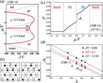
Figure 1: (color online) (a) The CMF-10 result for the ground-state phase diagram of hard-core bosons with nearest-neighbor repulsion on a triangular lattice in the ($J/V,\mu/V$)-plane, where second and first-order phase transitions are indicated by thin blue and thick red lines, respectively. (b) Schematic pictures of the symmetries of $\rho=2/3$ solid and upper SS states (left) and of $\rho=1/3$ solid and lower SS states (right). The lattice sites are separated into triangular (A) and honeycomb (B) sublattices. (c) The filling factor $\rho$ as a function of $\mu/V$ for $J/V=0.1$. (d) Cluster-size scaling ($\lambda\rightarrow 1$) of the CMF data for the jump $\Delta_{1}$ in $\rho$ at $\mu/V=3$. The linear fits of the three points ($N_{\rm C}=6$, $10$, and $15$) are fairly good.

To study the quantum melting transitions and the accompanying hysteresis curves, we use a cluster mean-field (CMF) method oguchi-55 ; hassan-07 ; yamamoto-09 ; EPAPS , in which we can easily get the stationary points of the free energy not only for the globally stable state but also for metastable and unstable states. To get meaningful results, one has to employ a sufficiently large cluster for estimating the values of mean fields. Although the use of the three-site cluster hassan-07 is convenient for tripartite lattices, the size $N_{\rm C}=3$ is too small to see clearly the effects of strong quantum fluctuations. The work described in Ref. hassan-07 failed to capture some important features of the phase diagram, e.g., the existence of the direct solid-SF transition at $1/3<\rho<2/3$ and the discontinuity of the SS-SF transition which will be mentioned later. Therefore, using much larger-size clusters of triangular shape (up to $N_{\rm C}=15$), here we perform more complex, but more reliable, calculations EPAPS .

To develop some intuition, we consider first hard-core bosons with only nearest neighbor interactions, i.e., we set $V_{jl}=V$ for nearest-neighbor bonds, and $V_{jl}=0$ otherwise. The ground-state phase diagram of this simplified model contains a wide region of SS phase, in which long-range solid (crystalline) order and superfluidity coexist, as well as the standard SF and solid phases murthy-97 ; boninsegni-05heidarian-05sen-08heidarian-10 ; wessel-05 . Figure 1(a) shows the ground-state phase diagram obtained by the ten-site CMF calculation (CMF-10). The SF state is characterized by the order parameter $\Psi\equiv\sum_{j}\langle\hat{a}_{j}\rangle/M$, where $M$ denotes the number of lattice sites. The solid states with filling factors $\rho=1/3$ and $\rho=2/3$ have the two-subblatice structures depicted in Fig. 1(b), which are characterized by $\rho_{\bf Q}\equiv\sum_{j}\langle\hat{n}_{j}\rangle\exp(i{\bf Q}\cdot{\bf r}_{j})/M$ with ${\bf Q}=(4\pi/3d,0)$. The filling factor is given by $\rho\equiv\sum_{j}\langle\hat{n}_{j}\rangle/M$. In the SS states, $|\Psi|$ and $|\rho_{\bf Q}|$ have non-zero values simultaneously. We determined the boundary lines of first-order transitions from the Maxwell construction in ($J/V,\chi$)-plane, where $\chi\equiv\sum_{\langle j,l\rangle}\langle\hat{a}^{\dagger}_{j}\hat{a}_{l}+\hat{a}^{\dagger}_{l}\hat{a}_{j}\rangle/M.$

In Fig. 1(c) we show the CMF-10 result for the filling factor $\rho$ as a function of $\mu/V$ along the line of $J/V=0.1$. At the particle-hole symmetry point $\mu/V=3$, we can obviously see a finite jump, $\Delta_{1}\approx 0.1$ for $J/V=0.1$, in the density curve, whereas previous numerical studies have shown that the density deviation $|\rho-1/2|$ at $\mu/V=3$ is extremely small or even undetectable boninsegni-05heidarian-05sen-08heidarian-10 ; wessel-05 . To examine this quantitative difference, we perform the infinite-size extrapolation of the results for different-size clusters [see Fig. 1(d)] with the scaling parameter $\lambda$ defined by $N_{\rm B}/(N_{\rm C}\times z/2)$, where $N_{\rm B}$ is the number of bonds within the cluster and $z=6$ (see Ref. EPAPS ). The jump $\Delta_{1}$ decreases with cluster size as expected. For example for $J/V=0.1$, its value is strongly reduced from $\Delta_{1}\approx 0.1$ of CMF-10 to $\Delta_{1}\approx 0.01$ in the limit $\lambda\rightarrow 1$. The extrapolated value vanishes at $J/V=0.108$, which means that the location of the triple point of the two SS and SF phases is shifted to $(J/V,\mu/V)=(0.108,3)$ in $\lambda\rightarrow 1$.

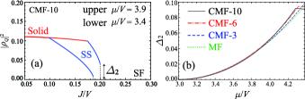
Figure 2: (color online) (a) The $J/V$ dependence of $|\rho_{\bf Q}|^{2}$ at $\mu/V=3.4$ and $\mu/V=3.9$. (b) The jump $\Delta_{2}$ in $|\rho_{\bf Q}|^{2}$ along the SS-SF (or solid-SF) transition line as a function of $\mu/V$.

The features of the phase diagram in Fig. 1(a) are in excellent agreement with those of QMC calculations wessel-05 . However, there is one major qualitative difference; our CMF results show that the transition between SF and SS is first-order (discontinuous). To confirm this, we plot $|\rho_{\bf Q}|^{2}$ as a function of $J/V$, calculated by CMF-10 along the horizontal lines $\mu/V=3.4$ and $\mu/V=3.9$, in Fig. 2(a). For the both values of $\mu/V$, there is a finite discontinuous jump $\Delta_{2}$ at the SS-SF transition, although that of the former is very small. The magnitude of jump decreases monotonically as the value of $\mu/V$ approaches the particle-hole symmetry point. It vanishes at $\mu/V=3$. As shown in Fig. 2(b), the curve shows very little change with increasing cluster size, and thus we conclude that the SS-SF transition is first-order except for the critical point $\mu/V=3$. In contrast, this transition seems to be continuous in QMC simulations, see Fig. 8 of Ref. wessel-05 , where the authors concluded that the SS-SF transition is second-order. This discrepancy may come from a finite-size effect of QMC calculations, since the magnitude of the jump $\Delta_{2}$ near $\mu/V=3$ is quite small as shown in Fig. 2(a). For values of $\mu/V$ farther away from the particle-hole symmetry line $\mu/V=3$, the discontinuous behavior is more pronounced, as shown in Fig. 2(b), and can now be observed also within QMC Note .

Let us discuss the hysteresis in the cycle of decreasing and increasing the chemical potential $\mu/V$. The system exhibits different hysteretic behaviors in three different ranges of $J/V$, which are defined by the thresholds $(J/V)_{\rm c1}\approx 0.182$, $(J/V)_{\rm c2}\approx 0.186$, and $(J/V)_{\rm c3}\approx 0.220$ [marked by the dashed vertical lines in Fig. 3(a)].

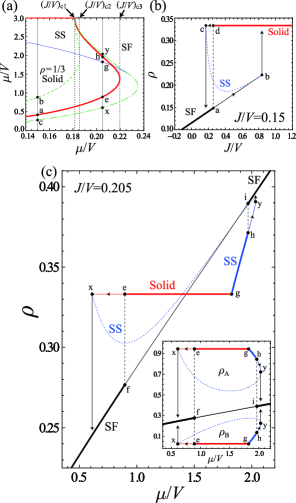
Figure 3: (color online) (a) Magnified view of the low-density regions of Fig. 1(a). We plot the limits of metastability of the SF phase (dashed green line) and the SS or solid phase (dash-dotted green line) in addition to the phase transition lines (thin blue and thick red lines) already shown in Fig. 1(a). (b) The usual hysteresis-loop and (c) anomalous unidirectional hysteresis behaviors. The thick solid, thin solid, and dashed lines represent ground, metastable, and unstable states, respectively. The inset in panel (c) shows the average density on each sublattice denoted by $\rho_{\rm A}$ and $\rho_{\rm B}$, which satisfy the relation $\rho=(\rho_{\rm A}+2\rho_{\rm B})/3$. The corresponding points in the figures are marked with the same letters.

In the first region, $J/V<(J/V)_{\rm c1}$, accompanying the SF-solid transition, a typical hysteresis loop is formed in the ($\mu/V,\rho$)-plane as indicated by the arrows in Fig 3(b). This is simply analogous to a conventional liquid-solid transition. In the second region, $(J/V)_{\rm c1}<J/V<(J/V)_{\rm c2}$, another hysteresis loop is formed around the SS-SF first-order transition point in addition to the loop around the SF-solid transition.

Of particular interest is the third region, $(J/V)_{\rm c2}<J/V<(J/V)_{\rm c3}$, in which the hysteresis exhibits an $anomalous$ behavior. As an example, we show in Fig. 3(c) the solution curves of the CMF-10 self-consistent equation in the ($\mu/V,\rho$)-plane for $J/V=0.205$. There are two first-order transitions, namely, between the solid (at point e) and SF (f) states and between the SS (h) and SF (i) states. Although the solution branches corresponding to metastable SF and unstable SS states apparently cross, the two states at the intersection are not identical. This is clearly seen in the inset of Fig. 3(c), where we plot the sublattice densities. Thus the solution curves are completely separated into the line of SF solutions and the twisted closed curve consisting of solid and SS solutions. In this case, we have an irreversible quantum melting transition, and once the solid order is melted at $T=0$, it will remain melted. In this regime, the solid phases can be reached again only through thermal cycling.

To illustrate this, let us assume that the system is initially in a stable solid state located between points e and g in Fig. 3(c). When decreasing $\mu/V$, although a SF state becomes energetically favorable below point e, the solid state remains metastable until it reaches point x. Below point x, the system is destabilized into the true ground state (namely the SF state). If we increase $\mu/V$ from the solid state, the system first undergoes a continuous transition to the SS phase at point g, and then the metastable SS state is also destabilized into the SF state at point y. On the other hand, the situation drastically changes if we start from an initial state in the SF phase. We see in Fig. 3(c) that the globally stable SF solutions at low and high $\mu/V$ are connected by the line of metastable SF solutions, which means that the SF state is stable for $any$ $\mu/V$. Therefore, when we decrease or increase $\mu/V$ starting from a SF state, the system remains in the SF phase even if the value of $\mu/V$ enters the region where a SS or solid state has the lowest energy. Thus the transition in varying $\mu/V$ occurs only from the SS (or solid) to SF phase, and the hysteresis curve does not form a standard loop structure. Crucially, this behavior gets more pronounced and the region $(J/V)_{\rm c2}<J/V<(J/V)_{\rm c3}$ becomes wider as the cluster size $N_{\rm C}$ increases, which means the robustness of the anomalous hysteresis when $\lambda\rightarrow 1$.

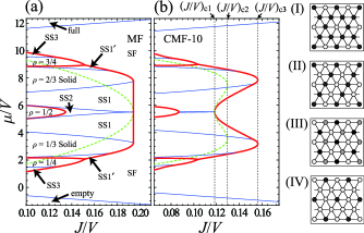
Figure 4: (color online) Ground-state phase diagram of hard-core bosons with full long-range dipole-dipole interactions on a triangular lattice in the ($J/V,\mu/V$)-plane, obtained from (a) MF theory and (b) CMF-10 method. Second and first-order phase transitions are indicated by thin blue and thick red lines, respectively. The dashed green lines represent the limit of metastability of the SF phase. The SS1 and SS1’ phases have the same sublattice structure as the SS phase in Fig. 1(b). (I-IV) Sublattice structures of the $\rho=3/4$ solid and the nearby SS3 (I), of the $\rho=1/2$ solid (II), of the SS2 (III), and of the $\rho=1/4$ solid and the nearby SS3 (IV).

We also discuss the influence of the full long-range dipole-dipole interactions sansone-10danshita-10 on our results. First, we perform a simple mean-field (MF) analysis for Eq. (1) with $V_{jl}=Vd^{3}/\left|{\bf r}_{j}-{\bf r}_{l}\right|^{3}$. As in the case of the nearest-neighbor interaction model, the MF phase diagram depicted in Fig. 4(a) includes large regions of $\rho=1/3$ and $\rho=2/3$ solids and the two-sublattice SS phase (named SS1) located between them. This is consistent with recent QMC calculations pollet-10 . Furthermore, the two-sublattice SS phase is stabilized also in the regions $\rho<1/3$ and $\rho>2/3$ (SS1’), and we find additional SS phases (SS2 and SS3) and solid phases with $\rho=1/2$, $\rho=1/4$, and $\rho=3/4$ within the parameter range of Fig. 4(a). To represent these phases, we allowed for three- and four-sublattice structures in minimizing the MF energy. Next, using the CMF-10 method we take into account quantum fluctuations around the MF solutions [see Fig 4(b)]. As in the case of nearest-neighbor interactions [Fig 1(b)], a noteworthy consequence of quantum fluctuations is that the SS1-SF boundary forms a dip around the particle-hole symmetry line. Moreover, a similar anomalous hysteresis described in the nearest-neighbor case also emerges here, and it is associated with the presence of the dip when $(J/V)_{\rm c2}<J/V<(J/V)_{\rm c3}$ [$(J/V)_{\rm c2}\approx 0.130$ and $(J/V)_{\rm c3}\approx 0.156$].

Actual experiments of ultracold gases are performed in the presence of a trap potential, e.g., $V_{t}({\bf r})=m\omega^{2}|{\bf r}|^{2}/2$. Within the local-density approximation (LDA), the effective local chemical potential is given by $\tilde{\mu}_{j}=\mu-V_{t}({\bf r}_{j})$. We suggest that the anomalous hysteretic behavior can be confirmed by controlling (decreasing and increasing) $\tilde{\mu}_{j}$ at the trap center via manipulation of, e.g., the frequency $\omega$ of the harmonic trap confining the dipolar gases. However, further analyses beyond LDA are still required to fully understand the behavior of the anomalous hysteresis in a trapped system.

In summary, we have studied phase transition phenomena in a system of dipolar Bose gases loaded into a triangular optical lattice. Using a CMF method, we have found that the first-order transition between the SS (or solid) and SF phases can exhibit an anomalous hysteretic behavior: in varying the chemical potential, the standard hysteresis loop structure does not appear, and the phase transition occurs only from the SS (or solid) to SF state. This unidirectional character is not predicted within the MF (classical) approach, since the boundary of the SS-SF transition is given by a straight line murthy-97 . Moreover, previous studies on a similar hard-core boson model with nearest-neighbor interactions for a square lattice have given only a standard hysteresis-loop behavior batrouni-00 . Thus, the anomalous feature of the hysteresis in this system is attributed to the interplay between quantum fluctuations and the competition of interactions due to the frustrated geometry of the triangular lattice.

More specifically, the most important point for the anomalous hysteresis behavior to emerge is the existence of the first-order SF-solid-(SS-)SF transition under varying $\mu/V$, as can be seen from Figs. 3(a) and (c). Thus we expect to find analogous anomalous hysteresis in a wide range of systems exhibiting $re$-$entrant$ first-order transitions (unless the system has no special symmetry point, e.g., the Heisenberg point in the square-lattice case batrouni-00 ). Recently, it has been suggested that $a$ $spin$ $supersolid$ $state$ can be realized in some magnetic systems mag . Thus, by analogy, we also expect that such quantum spin systems will exhibit a similar anomalous hysteresis behavior as a function of magnetic field.

We thank Grant-in-Aid from JSPS (D.Y.), KAKENHI (22840051) from JSPS (I.D.) and ARO (W911NF-09-1-0220) (C.S.d.M.) for support.

.1 Supplementary Material for “Dipolar Bosons in Triangular Optical Lattices:
Quantum Phase Transitions and Anomalous Hysteresis”

.2 A. A large-size CMF method and cluster-size scaling

The CMF method is convenient and effective in understanding the physics of ordered states including metastability phenomena since all stationary points of the free energy can be obtained not only for the globally stable solution. Moreover, this method is free from “finite-size effects” and “error bars.” However, in order to get reasonable results, one has to treat sufficiently large clusters as a reference system, especially when strong fluctuations exist in the system. In this work, we have used a series of clusters of $N_{\rm C}=3$, 6, 10, and 15 sites given in Table SI.

Table SI: A series of clusters used in our calculations. The values of $N_{\rm C}$, $N_{\rm B}$, and $\lambda$ are also listed.

	MF	CMF-3	CMF-6
$N_{\rm C}$	1	3	6
$N_{\rm B}$	0	3	9
$\lambda$	0	1/3	1/2
	CMF-10	CMF-15	Exact
$N_{\rm C}$	10	15	$\infty$
$N_{\rm B}$	18	30	$\infty$
$\lambda$	3/5	2/3	1

For a large cluster, we cannot calculate the value of free energy of the system directly from the CMF formalism, unlike the standard MF theory. This is a important problem for the system considered in this work, which exhibits first-order phase transitions in a wide region of parameters. To overcome this problem, we have used the Maxwell construction in ($J/V,\chi$)-plane to determine the phase boundary. The quantity $\chi$ is defined by $\chi\equiv\sum_{\langle j,l\rangle}\langle\hat{a}^{\dagger}_{j}\hat{a}_{l}+\hat{a}^{\dagger}_{l}\hat{a}_{j}\rangle/M,$ and the energy difference between the states at $J_{0}$ and $J_{1}$ (when $\mu$ and $V$ are fixed) is given by $-\int_{J_{0}}^{J_{1}}\chi(J)dJ.$ Note that the Maxwell construction in ($\mu/V,\rho$)-plane batrouni-00a is inapplicable in this case because of, indeed, the existence of the $anomalous$ hysteresis; as shown in Fig. 3(c), the solution curves are separated into two groups for $(J/V)_{\rm c2}<J/V<(J/V)_{\rm c3}$, and thus one cannot estimate the energy difference between states of different groups by using the integration of the density $\rho$ over the chemical potential $\mu/V$.

Moreover, to estimate the expectation values $\langle\cdots\rangle$, one should take the average not only over all internal sites within the cluster, but also all possible choices of how to embed the cluster itself in the background sublattice structure. For example, when we assume the two-sublattice $\sqrt{3}\times\sqrt{3}$ ordering in the ten-site CMF approximation (CMF-10), we have three choices of clusters shown in Fig. S1.

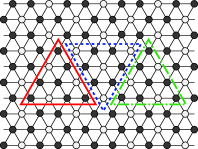
Figure S1: Schematic picture of the ten-site clusters embedded in the background two-sublattice $\sqrt{3}\times\sqrt{3}$ structure.

While we treat exactly the interactions within the cluster, the interactions between the cluster and the rest of the system are also included via effective fields acting at the cluster edge. The effective fields are determined self-consistently via the expectation values of the operators $\langle\hat{a}_{j}\rangle$ and $\langle\hat{n}_{j}\rangle$, in a standard manner CMFa .

In the main text, we have performed a cluster-size scaling of the CMF results for the amplitude of a discontinuous jump $\Delta_{1}$ at the transition between the two SS phases [see, Fig. 1(d)]. To extrapolate the value of $\Delta_{1}$, we introduced the scaling parameter $\lambda$ defined by $N_{\rm B}/(N_{\rm C}\times z/2)$, which varies from $0$ to $1$. Here, $N_{\rm B}$ is the number of bonds within the cluster and $z$ is the coordination number for the lattice, i.e., $z=6$ in this case. The denominator means the number of bonds of the original lattice per $N_{\rm C}$ sites, and hence the parameter $\lambda$ provides an indication of how much the correlation effects between particles are taken into account in the cluster. The value of $\lambda$ for each cluster is shown in Table SI. In Fig. 1(d) we performed a linear extrapolation toward $\lambda=1$ using the three points of CMF-6, -10, and -15, since the three-site cluster is too small for scaling. The linear fits of these three points are fairly good, as seen in Fig. 1(d). At $J/V=0.108$, the jump $\Delta_{1}$ vanishes in the limit $\lambda\rightarrow 1$, which means that the triple point of the two SS phases and the SF phase is strongly reduced from the MF value $J/V=0.25$ murthy-97a to $J/V=0.108$ due to the quantum fluctuations. This estimate for the triple point is in fairly good agreement with the recent QMC prediction bonnes-11a .

.3 B. Additional data for the transition between two SS phases

In the main text, we made only a passing reference to the transition between the high-density SS phase (often called SSA for distinction) and the low-density SS phase (SSB), since the main focus was the hysteresis occurring near the transition between solid (or SS) and SF phases. We present here some additional results for the properties of the SSA-SSB transition.

In Figs. S2(a-d), the results of the CMF-10 for the filling factor $\rho$, the solid order parameter $|\rho_{\bf Q}|$ with ${\bf Q}=(4\pi/3d,0)$, and the SF order parameter $|\Psi|$ are shown as functions of $\mu/V$ for $J/V=0.1$.

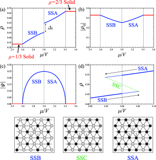
Figure S2: The $\mu/V$ dependences of (a) the average density $\rho$, (b) the solid order parameter $|\rho_{\bf Q}|$, and (c) the SF order parameter $|\Psi|$ for $J/V=0.1$, obtained by the CMF-10 calculations. (d) Magnified view of the region near $\mu/V=3$ in (a). The thick solid, thin solid, and dashed lines represent the solutions of the ground, metastable, and unstable states, respectively. The lower panels show the sublattice structures of SSA, SSB, and SSC.

As shown in Fig. S2(a), the ground-state density curves of SSA and SSB are not connected at the center, while the two order parameters in Figs. S2(b) and (c) do not show such discontinuity. The latter is because of the particle-hole symmetry at $\mu/V=3$. The discontinuity in the density indicates the first-order character of the transition between the two SS phases, although the amplitude of the jump is strongly reduced in the limit $\lambda\rightarrow 1$ [see, Fig. 1(d)].

In addition, we plot in Fig. S2(d) the solution curve of the CMF-10 equation, including the metastable and unstable solutions, near the SSA-SSB phase boundary. The solution lines of SSA and SSB are extended due to the metastability, and connected by the line of the three-sublattice SS state, called SSC wessel-05a ; boninsegni-05a ; sen-08a ; heidarian-10a . We found that unstable SSC solutions (corresponding to unstable stationary points of the free energy) exist in the vicinity of half filling, although there is no region of the SSC phase in the ground-state phase diagram. The density versus chemical potential curve has negative curvature (negative compressibility) in the SSC state, which indicates the emergence of phase separation at a fixed density near $\rho=1/2$; the system separates into a mixture of SSA and SSB phases.

Note that in the case of infinite-range dipole-dipole interactions, there is a finite region of stable SSC phase in the phase diagram (marked SS2 in Fig. 4), although it is remarkably narrow for CMF-10. It is an interesting future issue to determine whether the SSC phase is actually stable or not for the infinite-range interaction model.

References

- (1) A. Griesmaier ., Phys. Rev. Lett. 94, 160401 (2005).
- (2) T. Lahaye ., Nature (London) 448, 672 (2007).
- (3) K.-K. Ni ., Science 322, 231 (2008).
- (4) S. Ospelkaus ., Faraday Discuss. 142, 351 (2009).
- (5) K. Aikawa ., Phys. Rev. Lett. 105, 203001 (2010).
- (6) C. Becker ., New J. Phys. 12, 065025 (2010).
- (7) J. S. Gardner ., Phys. Rev. Lett. 83, 211 (1999).
- (8) L. Balents, Nature (London) 464, 199 (2010).
- (9) S. T. Bramwell ., Phys. Rev. Lett. 87, 047205 (2001).
- (10) H. Matsuda and T. Tsuneto, Suppl. Prog. Theor. Phys. 46, 411 (1970).
- (11) L. Pollet ., Phys. Rev. Lett. 104, 125302 (2010).
- (12) T. Oguchi, Prog. Theor. Phys. 13, 148 (1955).
- (13) S. R. Hassan, L. de Medici, and A.-M. S. Tremblay, Phys. Rev. B 76, 144420 (2007).
- (14) H. A. Bethe, Proc. R. Soc. London, Ser. A 150, 552 (1935); D. Yamamoto, Phys. Rev. B 79, 144427 (2009).
- (15) See the supplementary material attached below.
- (16) G. Murthy, D. Arovas, and A. Auerbach, Phys. Rev. B 55, 3104 (1997).
- (17) M. Boninsegni and N. Prokof’ev, Phys. Rev. Lett. 95, 237204 (2005); D. Heidarian and K. Damle, Phys. Rev. Lett. 95, 127206 (2005); R. G. Melko ., Phys. Rev. Lett. 95, 127207 (2005); A. Sen ., Phys. Rev. Lett. 100, 147204 (2008); D. Heidarian and A. Paramekanti, Phys. Rev. Lett. 104, 015301 (2010).
- (18) S. Wessel and M. Troyer, Phys. Rev. Lett. 95, 127205 (2005).
- (19) After the release of the preprint version of this Letter, this prediction has been confirmed by QMC [L. Bonnes and S. Wessel, Phys. Rev. B 84, 054510 (2011); X.-F. Zhang ., . 84, 174515 (2011)].
- (20) B. Capogrosso-Sansone ., Phys. Rev. Lett. 104, 125301 (2010); I. Danshita and D. Yamamoto, Phys. Rev. A 82, 013645 (2010).
- (21) G. G. Batrouni and R. T. Scalettar, Phys. Rev. Lett. 84, 1599 (2000).
- (22) K.-K. Ng and T. K. Lee, Phys. Rev. Lett. 97, 127204 (2006); P. Sengupta and C. D. Batista, Phys. Rev. Lett. 98, 227201 (2007).

References

- (1) G. G. Batrouni and R. T. Scalettar, Phys. Rev. Lett. 84, 1599 (2000).
- (2) T. Oguchi, Prog. Theor. Phys. 13, 148 (1955); H. H. Chen and F. Lee, Phys. Rev. B 48, 9456 (1993); A. J. García-Adeva and D. L. Huber, Phys. Rev. Lett. 85, 4598 (2000); S. R. Hassan, L. de Medici, and A.-M. S. Tremblay, Phys. Rev. B 76, 144420 (2007).
- (3) G. Murthy, D. Arovas, and A. Auerbach, Phys. Rev. B 55, 3104 (1997).
- (4) L. Bonnes and S. Wessel, Phys. Rev. B 84, 054510 (2011).
- (5) M. Boninsegni and N. Prokof’ev, Phys. Rev. Lett. 95, 237204 (2005).
- (6) S. Wessel and M. Troyer, Phys. Rev. Lett. 95, 127205 (2005).
- (7) A. Sen, P. Dutt, K. Damle and R. Moessner, Phys. Rev. Lett. 100, 147204 (2008).
- (8) D. Heidarian and A. Paramekanti, Phys. Rev. Lett. 104, 015301 (2010).