Quantum Monte Carlo calculation of the zero-temperature phase diagram of the two-component fermionic hard-core gas in two dimensions

Abstract

Motivated by potential realizations in cold-atom or cold-molecule systems, we have performed quantum Monte Carlo simulations of two-component gases of fermions in two dimensions with hard-core interactions. We have determined the gross features of the zero-temperature phase diagram, by investigating the relative stabilities of paramagnetic and ferromagnetic fluids and crystals. We have also examined the effect of including a pairwise, long-range $r^{-3}$ potential between the particles. Our most important conclusion is that there is no region of stability for a ferromagnetic fluid phase, even if the long-range interaction is present. We also present results for the pair-correlation function, static structure factor, and momentum density of two-dimensional hard-core fluids.

I Introduction

Ultracold gases of fermionic atoms and molecules have been the subject of a large number of experimental and theoretical studiesblochdz ; giorgini in the last decade. The interest in these systems arises from the fact that the atoms or molecules obey quantum statistics rather than classical statistics and exhibit interesting and novel quantum phases at sufficiently low temperatures. Unlike electron systems, it is possible to manipulate the interaction between the atoms or molecules to some extent, e.g., by Feshbach resonanceschin_2010 and/or by applying microwave fields.papoular ; innsbruck ; gorshkov_2008 ; cooper_2009 The ability to control the interactions can be used to gain insight into the physics of phase transitions and the nature of correlation effects in these quantum phases. Celebrated examples are the experimental studies of the Mott transition for bosonsgreiner and of the superfluid pairing in the unitary (strong-coupling) Fermi gas.blochdz ; giorgini Finally, ultracold atomic gases may play an important role in future quantum computing devices.

Recently, interest has turned towards the use of ultracold atomic systems to investigate ferromagnetism in Fermi gases. Itinerant ferromagnetism in electron systems is poorly understood, and it is possible that insights might be gained by studying ferromagnetic fluid states in cold-atom systems.duine Experimental studies of strongly repulsive Fermi gases close to Feshbach resonances have found behavior consistent with the formation of (local) ferromagnetic correlations in the manner of Stoner ferromagnetism.ketterle However, these systems are limited by an intrinsic instability to molecule formation, which results in a short lifetime for the ferromagnetic state and may also complicate the interpretation of experimental features.pekker ; babadi It is therefore of interest to explore other forms of interaction that might give rise to ferromagnetism in the absence of nearby bound states.

An interesting class of experimental system in this regard is provided by gases of fermionic polar molecules (e.g., ⁴⁰K⁸⁷Rb or ⁷Li⁴⁰K). Polar molecules that are confined to two-dimensional (2D) layers and dressed by a circularly polarized microwave field experience a long-range potential that falls off as $r^{-3}$, where $r$ is the intermolecular distance.innsbruck ; gorshkov_2008 ; cooper_2009 Furthermore, the dressed states have the feature that there is a very sharp increase in the potential energy at short distances, preventing close approach. Hence such molecules can be modeled as a gas of fermionic hard-core particles with an additional long-range potential varying as $r^{-3}$. The hard-core potential prevents the formation of shallow bound states even for (weakly) attractive long-range interactions. It has been suggested that a single-component gas of such fermionic molecules will exhibit a topological superfluid $p$-wave pairing phase, of direct relevance to possible topologically protected quantum computing devices.cooper_2009 ; nayak_2008

Here we consider the case of a two-component gas of such fermionic molecules. We have applied quantum Monte Carlo (QMC) methods to address the issue of whether or not the hard-core interactions cause this system to exhibit a region of itinerant ferromagnetism. In particular we have used the variational and diffusion quantum Monte Carlo (VMC and DMC) techniquesceperley_1980 ; foulkes_2001 to establish the ground-state phase diagram of two-component gases of fermionic hard-core particles moving in 2D. QMC methods are widely acknowledged to be the most accurate first-principles techniques available for studying condensed matter. In the VMC method, Monte Carlo integration is used to evaluate expectation values with respect to an explicitly correlated many-body trial wave function. In the DMC method, the ground-state component of a trial wave function is projected out by a stochastic algorithm. Fermionic symmetry is maintained by the fixed-node approximation.anderson_1976

Some of the earliest applications of QMC methods were to study the ground-state properties of bosonic hard-sphere fluids, as a model for the behavior of ⁴He.liu_1973 ; demichelis_1978 ; lei_1990 More recently, QMC methods have been used to study 3D fermionic systems in which there is a hard-sphere repulsion between opposite-spin particles.chang_2010 ; pilati_2010 To the best of our knowledge, however, QMC methods have never previously been used to study the phase diagram of 2D gases of fermionic hard-core particles

This paper is arranged as follows. In Sec. II we describe the model Hamiltonian that we study. In Sec. III we discuss the form of trial wave function that we use. In Sec. IV we consider the issue of finite-size errors and explain how we extrapolate to the thermodynamic limit. In Sec. V we present our results for the phase diagram of fermionic hard-core particles and in Sec. VI we present results for the pair-correlation function (PCF), static structure factor, and momentum density of hard-core fluids. In Sec. VII we investigate whether the inclusion of weak, long-range interactions affects the phase diagram. Finally, we draw our conclusions in Sec. VIII. All our QMC calculations were performed using the casino code.casino

II Hard-core model

II.1 Hard-core Hamiltonian

Suppose we have a system of interacting, circular hard-core particles moving in two dimensions. Throughout, we use units (a.u.) in which the Dirac constant, the mass of the particles, and the radius of the circle that contains one particle on average are unity. We assume the particles to be fermions with spin $s=1/2$. Let $D$ be the diameter of the particles. In these units the Hamiltonian is

$$\hat{H}=\sum_{i}-\frac{1}{2}\nabla_{i}^{2}+\sum_{i>j}v_{H}(r_{ij}),$$ (1)

where

$$v_{H}(r)=\left\{\begin{array}[]{ll}0&{\rm if}~{}r>D\\ \infty&{\rm otherwise}\end{array}\right..$$ (2)

When we refer to “high density,” we mean that the value of $D$ is large (comparable with the radius of the circle that contains one particle on average). In our calculations we used finite numbers $N$ of particles in cells subject to periodic boundary conditions. From these we extrapolated to infinite system size, as discussed in Sec. IV.

The potential energy is zero throughout the permitted region of configuration space. Hence the expected potential energy is zero, and the system only has kinetic energy. Nevertheless, the hard-core interaction has a significant effect on the energy, since it defines the boundary conditions on the solution of the Schrödinger equation. Hence the system does not behave like a noninteracting Fermi gas: the magnetic behavior is nontrivial and the system must crystallize at a sufficiently high density.

Hard-core systems have a maximum density: the close-packing limit. In 2D the triangular lattice has the highest packing fraction, with the maximum hard-core diameter being $D_{\rm max}=\sqrt{2\pi/\sqrt{3}}$.

II.2 Qualitative features of the phase diagram

For infinitesimal $D$, the system resembles a noninteracting Fermi gas. The momentum density is a unit step function. The paramagnetic fluid phase is favored, because it has the lowest kinetic energy. The crystal is not even stable as an excited state for small $D$.

As $D$ is increased, the energy of the paramagnetic fluid rises more rapidly than that of the ferromagnetic fluid, because wave-function antisymmetry already keeps parallel-spin particles apart. The hard-core interactions have a greater effect on the distribution of antiparallel-spin particles, with the short-range PCF being forced to go to zero, as shown in Sec. VI.1. The momentum density of a hard-core fluid with $D>0$ is not a unit step function, but it retains a discontinuity at the Fermi wave vector $k_{F}$. The crystal becomes stable as $D$ is increased, but with a higher energy than that of the fluid.

At large $D$, the energies of the ferromagnetic and (frustrated) antiferromagnetic crystals are very similar. At some value of $D$ the ferromagnetic fluid is lower in energy than the paramagnetic fluid, but at some other value of $D$ the crystal becomes more stable than either of the fluid phases. It is a nontrivial problem to determine which of these transitions occurs first. The crystal orbitals become delta functions in the close-packing limit.

III Trial wave functions

III.1 Slater-Jastrow-backflow wave functions

We used trial wave functions of Slater-Jastrow-backflow form $\Psi=\exp(J)S^{\uparrow}S^{\downarrow}$. The Jastrow exponent $J$ included polynomial and plane-wave functions of the interparticle distancesndd_jastrow together with a two-body term to impose the hard-core boundary conditions, as described in Sec. III.2, and a three-body term.casino_manual The backflow function consisted of a polynomial expansion in the interparticle distance.backflow The terms in the Jastrow exponent and backflow function arising from parallel-spin and antiparallel-spin pairs of particles were allowed to differ.

Plane-wave orbitals $\exp(i{\bf k}\cdot{\bf r})$ were used in the Slater determinants $S^{\uparrow}$ and $S^{\downarrow}$ for the fluid phases. The fluid phases suffer from momentum quantization effects (single-particle finite-size errors). To reduce these, we performed twist averaging in the canonical ensemble.lin_twist_av

We used Gaussian orbitals $\exp\left(-C|{\bf r}-{\bf R}_{p}|^{2}\right)$ centered on hexagonal lattice sites $\{{\bf R}_{p}\}$, where the exponent $C$ in the crystal orbitals is an optimizable parameter, for the crystal phases.

These calculations are similar to the QMC calculations that have been performed to establish the zero-temperature phase diagram of the three dimensional homogeneous electron gas (HEG)ceperley_1980 ; zong_2002 ; ndd_3d_heg and 2D HEG.tanatar ; rapisarda ; ndd_2d_heg

III.2 Hard-core two-body behavior

III.2.1 Antiparallel spins

Let us rewrite the Schrödinger equation for two hard-core particles in terms of the center-of-mass and difference coordinates. We assume the center of mass is in its zero-energy ground state. The Schrödinger equation for the difference coordinate ${\bf r}$ is

$$-\nabla^{2}\Psi=E\Psi.$$ (3)

For the boundary conditions we assume that $\Psi=0$ at $r=D$ and $\Psi=0$ at $r=R$, where $R$ is very large. By increasing $R$, the ground-state eigenvalue $E$ can be made arbitrarily close to 0. $\Psi$ is circularly symmetric in the ground state for antiparallel-spin particles, so

$$-\frac{\partial^{2}\Psi}{\partial r^{2}}-\frac{1}{r}\frac{\partial\Psi}{\partial r}\approx 0,$$ (4)

with general solution $\Psi\approx A+B\log(r)$. This approximation is valid over any range of $r$ that is small compared with $R-D$. However, we are interested in particle separations of the order $D$ and slightly larger. Applying the boundary condition $\Psi(D)=0$ gives

$$\Psi(r)\propto\log(r/D),$$ (5)

suggesting the antiparallel-spin two-body Jastrow factor in a hard-core gas should be $\log(r/D)$.

The two-body behavior of hard-core gases was studied in Ref. li, , but this work did not give the two-body Jastrow factor for the 2D gas and did not consider parallel-spin pairs.

III.2.2 Parallel spins

Suppose the two hard-core particles have parallel spins. In the lowest-energy state the difference-coordinate wave function is of the form $\Psi=W(r)r\cos(\theta)$ and the energy eigenvalue is zero in the limit that the region over which the wave function is normalized is large. Hence the Schrödinger equation for the radial part is

$$-\frac{d^{2}W}{dr^{2}}-\frac{3}{r}\frac{dW}{dr}\approx 0.$$ (6)

The general solution over a range of $r$ values that is small compared with the region over which the wave function is normalized is $W(r)\approx A+Br^{-2}$. Applying the boundary condition $W(D)=0$, one obtains $W(r)\propto 1-D^{2}/r^{2}$. So, for small $r$,

$$\Psi\propto\left(1-\frac{D^{2}}{r^{2}}\right)r\cos(\theta),$$ (7)

suggesting the parallel-spin two-body Jastrow factor in a hard-core gas should be $1-D^{2}/r^{2}$.

III.3 Hard-core Jastrow factor

The wave function of a hard-core system must go linearly to zero as the separation of any pair of particles approaches $D$. To impose this behavior, the following term was included between all pairs of particles in the Jastrow exponent $J$ (in addition to the polynomial and plane-wave terms):

$$u_{H}(r)=\left\{\begin{array}[]{ll}-\infty&{\rm if}~{}r\leq D\\ \log\left[\tanh\left(\frac{r/D-1}{\alpha(1-r/L_{\rm WS})}\right)\right]&{\rm if}~{}D<r<L_{\rm WS}\\ 0&{\rm if}~{}r\geq L_{\rm WS}\end{array}\right.,$$ (8)

where $L_{\rm WS}$ is the radius of the circle inscribed in the Wigner-Seitz cell of the simulation cell. The parameter $\alpha$ was fixed at 1. $u_{H}$ goes smoothly to zero at $L_{\rm WS}$. The other terms in the Jastrow factor are analytic at $r=D$.

$\exp(u_{H})\approx\tanh[(r-D)/D]$ is not of the form $\log(r/D)$ or $1-D^{2}/r^{2}$ suggested by the analytic results for opposite-spin or same-spin hard-core particles, respectively, but the short-range behavior is correct [linear in $(r-D)$ in the vicinity of $r=D$]. When optimized, the polynomial and plane-wave terms in the Jastrow exponent describe all two-body correlations. Optimized two-body Jastrow factors are plotted in Fig. 1, confirming that the simple theory of two-body correlations described in Sec. III.2 is approximately valid.

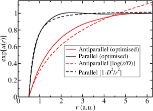
Figure 1: (Color online) Two-body Jastrow factors $\exp[u(r)]$ for $N=50$ paramagnetic hard-core particles with $D=0.5$ a.u.

III.4 Free-particle limit

It is interesting to consider the approach to the free-particle limit as the diameter $D$ tends to zero. In a three-dimensional hard-core gas, similar arguments to those given in Secs. III.2.1 and III.2.2 show that the two-body Jastrow factors are approximately $1-D/r$ and $1-D^{3}/r^{3}$ for antiparallel and parallel spins, respectively, both of which tend to unity as $D\rightarrow 0$. Hence a Slater-Jastrow wave function for a three-dimensional hard-core fluid reduces to a Slater determinant of plane-wave orbitals in the limit of zero particle diameter. In the 2D hard-core gas the two-body Jastrow factors are approximately $\log(r/D)$ and $1-D^{2}/r^{2}$ for antiparallel and parallel spins, respectively. The antiparallel-spin two-body Jastrow factor is the marginal case in which two-body correlations become negligible over any given length scale as $D$ is made small so that free-particle behavior is recovered in the $D\rightarrow 0$ limit. In one dimension, however, the infinite contact potential that remains when the $D\rightarrow 0$ limit is taken prevents the hard-core gas from exhibiting free-particle behavior, unless the system is fully ferromagnetic.

III.5 Behavior of the local energy as hard-core particles collide

Suppose two antiparallel-spin hard-core particles 1 and 2 approach each other, i.e., their separation approaches $D$. Their contribution to the Jastrow exponent is $J_{12}=\log(r_{12}-D)$. Let us write the trial wave function as $\Psi=\exp(J_{12})S$, where $S$ is well-behaved as the particles approach. Suppose that all coordinates in the system are frozen, apart from the separation of particles 1 and 2. The contribution to the local energy arising from this coordinate is

$$E_{L12} = -\frac{\nabla_{12}^{2}\Psi}{\Psi}$$ (9)

$$= |\nabla_{12}J_{12}|^{2}+\nabla_{12}^{2}J_{12}+2\nabla_{12}J_{12}\cdot\frac{\nabla_{12}S}{S}+\frac{\nabla_{12}^{2}S}{S}$$

$$= \frac{1}{r_{12}(r_{12}-D)}\left(1+2{\bf r}_{12}\cdot\frac{\nabla_{12}S}{S}\right)+\frac{\nabla_{12}^{2}S}{S}.$$

The local energy diverges when hard-core particles approach one another, and the sign of the divergence depends on the positions of all the particles. Hence one cannot remove the divergence using a two-body Jastrow factor. By contrast, when two charged point particles approach one another, the divergence in the local energy can be removed by imposing the Kato cusp conditions via the two-body Jastrow factor.kato_pack

The divergence is in principle no worse than that which occurs at any other node. However, there are many extra nodes introduced by the hard-core potentials, on which the local kinetic energy diverges. These nodes can cause DMC population explosions,umrigar_1993 especially if three-body terms are omitted from the Jastrow factor.

III.6 Need for a three-body Jastrow term

Physically, it is obvious that at high densities multi-body correlation effects will be important: motion is only possible if the particles move collectively. In fact, as shown in Table 1, three-body Jastrow terms lower the VMC energy more than backflow. This differs from the behavior found in the HEG.ndd_2dheg_expvals We have therefore used three-body terms in all our calculations. If the range of the three-body terms is restricted then the wave function becomes significantly poorer, as can be seen in Table 1. Unfortunately, the need to include long-range three-body terms in the Jastrow factor makes the calculations expensive.

Meth.	WF	SR BF	SR 3BJ	$E$ (a.u./part.)	Var. (a.u.)
VMC	SJ	–	–	$4.8242(4)$	$286$
VMC	SJB	F	–	$4.7172(9)$	$242$
VMC	SJB3	T	T	$4.6360(2)$	$160$
VMC	SJB3	F	T	$4.6272(1)$	$158$
VMC	SJ3	–	F	$4.58672(8)$	$89$
VMC	SJB3	T	F	$4.5201(2)$	$70$
VMC	SJB3	F	F	$4.5072(6)$	$65$
DMC	SJ	F	F	$4.4157(6)$	–
DMC	SJB	F	–	$4.4058(7)$	–
DMC	SJB3	F	F	$4.3930(8)$	–

Table 1: Non-twist-averaged VMC and DMC results with different wave functions (“WF”) for a paramagnetic fluid of $N=26$ hard-core particles of diameter $D=1$ a.u. The “SR BF” column specifies whether or not the backflow function was restricted to be short-ranged (cutoff length 2.5 a.u.), while the “SR 3BJ” column specifies whether or not the three-body Jastrow terms were restricted to be short-ranged (cutoff length 2.5 a.u.). Where the cutoff lengths were not restricted, they approached the radius of the circle inscribed in the Wigner-Seitz cell of the simulation cell. “T” and “F” denote true and false, while “Var.” is the variance of the local energy.

III.7 Spin-dependence in paramagnetic phases

We used separate two-body Jastrow and two-body backflow terms for parallel-spin and antiparallel-spin pairs of particles in all our calculations. We considered two possible spin-dependences for the three-body terms: either (A) using the same three-body term for all triples of particles or (B) using separate three-body terms for (i) triples involving three particles of the same spin and (ii) triples involving two particles of one spin and one particle of the opposite spin. VMC results obtained using these two different possibilities are shown in Table 2. It is clear that allowing different three-body terms for different spin configurations lowers the variational energy significantly (although not by nearly as much as lifting the restriction on the range of the three-body terms) and hence we have used spin-dependence B in all our production calculations.

Spin-dep.	SR BF & 3BJ	Energy (a.u./part.)	Var. (a.u.)
A	T	$4.640(1)$	$165$
B	T	$4.6360(2)$	$160$
A	F	$4.534(1)$	$76$
B	F	$4.5072(6)$	$65$

Table 2: Non-twist-averaged VMC results with different spin dependences for a paramagnetic fluid of $N=26$ hard-core particles of diameter $D=1$ a.u. The “SR BF & 3BJ” column specifies whether or not the backflow function and three-body Jastrow terms were restricted to be short-ranged (cutoff length 2.5 a.u.). Where the cutoff lengths were not restricted, they approached the radius of the circle inscribed in the Wigner-Seitz cell of the simulation cell. “T” and “F” denote true and false, while “Var.” is the variance of the local energy.

III.8 Relative accuracy of wave functions for different phases

The variance of the energy is zero if the trial wave function is an eigenfunction of the Hamiltonian. As shown in Table 3, the variance per particle is significantly lower for the ferromagnetic fluid than the paramagnetic fluid, indicating that the trial wave function is more accurate for the former than the latter. The variance per particle is similar for ferromagnetic fluids and crystals near the transition density. Hence, if anything, our results are biased in favor of ferromagnetic phases.

$D$ (a.u.)	Phase	Var. per part. (a.u.)
$1$	Para. fluid	$2.49$
$1$	Ferro. fluid	$1.76$
$1$	Ferro. crystal	$0.736$
$0.88$	Para. fluid	$1.34$
$0.88$	Ferro. fluid	$0.616$
$0.88$	Ferro. crystal	$0.494$
$0.63$	Para. fluid	$0.385$
$0.63$	Ferro. fluid	$0.147$
$0.63$	Ferro. crystal	$0.228$

Table 3: Non-twist-averaged VMC results for paramagnetic fluids with $N=26$ hard-core particles and ferromagnetic fluids with $N=25$ hard-core particles.

III.9 Nature of phase transition

We have looked for a first-order phase transition by comparing fixed-node DMC energies with fluid and crystal orbitals, relying on the fixed-node approximation to impose the symmetry of the phase on the wave function. However, it is possible that there could actually be a continuous transition from fluid to crystal behavior. The fact that the “fluid” wave function tries to become crystal-like at high density and the “crystal” wave function tries to become fluid-like at low density (see Sec. VI) supports this view. Nevertheless, even if this is the case, our calculations determine the region in which crystallization is expected to take place, and demonstrate that a ferromagnetic fluid phase is unlikely to occur.

IV Finite-size effects

According to the simple theory given in Sec. III.2.2, the long-range parallel-spin two-body Jastrow exponent is approximately given by

$$u_{\alpha\alpha}(r)=\log(1-D^{2}/r^{2})\approx-D^{2}/r^{2}+O(r^{-4}).$$ (10)

The 2D Fourier transform of the leading term does not have a power-law behavior. In fact numerical tests show that $\lim_{\alpha\rightarrow 0}\int r^{-2}\exp(i{\bf k}\cdot{\bf r}-\alpha r)\,d{\bf r}$ diverges logarithmically at small $k$. So, for small $k$, $u_{\alpha\alpha}(k)$ may be written as $-cD^{2}\log(k)$, where $c$ is a positive constant.

The Chiesa-Holzmann-Martin-Ceperleyfin_chiesa approximation to the long-range two-body finite-size correction to the kinetic energy in 2D is

$$\Delta T = -\sum_{\alpha}\frac{N_{\alpha}}{4(2\pi)^{2}}\int_{0}^{Q}2\pi k\times k^{2}u_{\alpha\alpha}(k)\,dk$$ (11)

$$= -\frac{N}{8\pi}\int_{0}^{Q}k^{3}u_{\alpha\alpha}(k)\,dk,$$

where $Q=2\sqrt{\pi/A}$ is the radius of the circle in ${\bf k}$-space with area $(2\pi)^{2}/A$ and $A=\pi N$ is the area of the simulation cell. Inserting $u_{\alpha\alpha}(k)=-cD^{2}\log(k)$ gives

$$\Delta T \approx \frac{\pi NcD^{2}}{2A^{2}}\left[\log\left(2\sqrt{\pi/A}\right)-4\pi^{2}/A^{2}\right]$$ (12)

$$= O[D^{2}N^{-1}\log(N)].$$

Hence, ignoring the logarithmic factor, the leading-order correction to the energy per particle due to the neglect of long-range two-body correlations falls off as $O(N^{-2})$. This is much more rapid than the analogous result for the 2D HEG.ndd_fs The leading-order correction is positive. Unsurprisingly, however, two-body finite-size errors get rapidly more severe as $D$ increases.

We have carried out numerical tests which show that the bias due to twist averaging in the canonical ensemble in two dimensions falls off as $O(N^{-3/2})$, but with a small prefactor. Residual single-particle errors in the canonical-ensemble twist-averaged fluid energies are small compared with the effect of twist averaging, and the difference between the twist-averaged and non-twist-averaged energies is only about 0.02 a.u. per particle at $D=1$ a.u. for $N=10$ and $26$. Hence the $O(N^{-2})$ behavior due to the neglect of long-range two-body correlations dominates the systematic error for all the hard-core diameters $D$ that we have studied, as can be seen in Fig. 2.

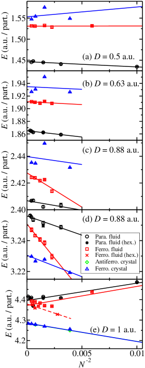
Figure 2: (Color online) DMC energy $E$ against the reciprocal of the square of the system size $N^{-2}$ for (a) $D=0.5$ a.u., (b) $D=0.63$ a.u., (c) $D=0.75$ a.u., (d) $D=0.88$ a.u., and (e) $D=1$ a.u.

Several data points in Fig. 2 are outliers. This nonsystematic behavior appears to be a genuine finite-size effect. The finite-size “noise” in the crystal energies is more severe at low densities, while the finite-size noise in the fluid energies is more severe at very high densities. The theory of two-body finite-size effects developed above breaks down for fluids at high density and crystals at low density: the sign of the bias is wrong. These cases are pathological in various respects. At very high densities, the fluid energies obtained with the same number of particles in different-shaped cells disagree, although they extrapolate to the same value in the limit of infinite system size. In fact at very high density it is geometrically impossible to fit finite fluids in some cell shapes. As can be seen in Fig. 3, the Gaussian exponent $C$ of the crystal is not well-behaved for $D\leq 0.75$, suggesting that the crystal is becoming unstable. As shown in Fig. 14, the momentum density is developing an edge, leading to substantial single-particle finite-size errors.

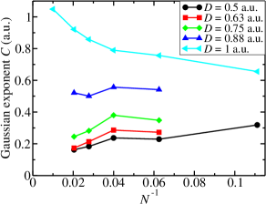
Figure 3: (Color online) Optimal Gaussian exponent $C$ for the ferromagnetic crystal phase against the reciprocal of system size $N^{-1}$.

As shown in Table 1, restricting the range of the three-body term raises the variational energy significantly. Three-body correlations are therfore long-ranged. So there must be three-body finite-size errors in the fluid and crystal energies obtained in finite simulation cells. We assume they are a “random” error about the systematic finite-size bias due to two-body finite-size effects. We have therefore obtained several $E(N)$ data points for each phase at each density in order to average out the “noise” when extrapolating to infinite system size.

V Phase diagram

The energies of the different phases are compared in Fig. 4 and are plotted relative to the energy of the paramagnetic fluid phase in Fig. 5. The continuous curves shown are Akima spline interpolations between the DMC energies. (Akima spline interpolation is stable to the presence of outliers in the data.akima ) It can be seen that crystallization takes place when $D=0.83$ a.u., leaving no region of stability for a ferromagnetic fluid. (Recall that our calculations are, if anything, biased in favor of the ferromagnetic fluid.) Thus our calculations rule out the possibility of an itinerant ferromagnetic fluid phase in a 2D gas of particles with only hard-core interactions. For those values of $D$ for which the crystal has the lowest energy, the energy difference between the antiferromagnetic and ferromagnetic states is insignificant, showing that exchange interactions in the crystalline phase are negligible.

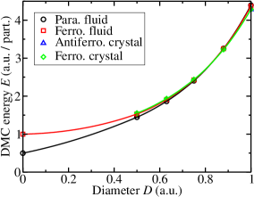
Figure 4: (Color online) DMC energy $E$ against hard-core diameter $D$. Note that, when $D=0$ the energies of the paramagnetic and ferromagnetic fluids are 0.5 and 1 a.u. per particle, respectively.

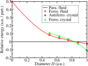
Figure 5: (Color online) DMC energy of the different phases relative to the energy of the paramagnetic fluid.

VI Other properties of hard-core gases

VI.1 Pair-correlation function

We have calculated the PCFs of the fluid phases of the hard-core gas, and our results are shown in Fig. 6. The PCFs, which were obtained without twist averaging, are not well-converged with respect to system size at high density: the finite-size errors are oscillatory. Nevertheless, we can make some qualitative comments about the physics revealed by the PCF.

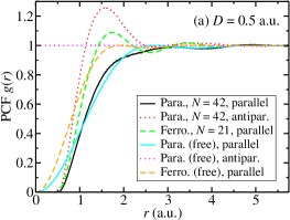
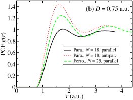
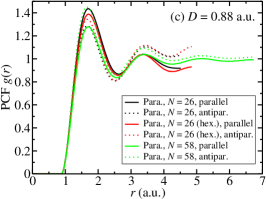
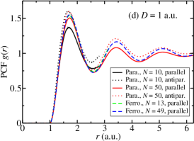
Figure 6: (Color online) VMC PCFs $g(r)$ of hard-core systems at (a) $D=0.5$ a.u., (b) $D=0.75$ a.u., (c) $D=0.88$ a.u., and (d) $D=1$ a.u., for different system sizes $N$.

The distance between the peaks of the PCF obtained in square cells at $D=1$ a.u. is $\sqrt{\pi}$, which arises from the square-cell geometry. The difference between the PCFs in hexagonal and square cells is still significant at $D=0.88$ a.u. and $N=26$. The antiparallel-spin PCF evolves slowly towards $g(r)=1$ (the free-particle result) as $D$ is reduced. The size of the exchange-correlation hole and the ripples in the parallel-spin PCF are determined by the Fermi wave vector $k_{F}$ when $D$ is small.

VI.2 Static structure factor

The static structure factor of a paramagnetic fluid at $D=0.63$ a.u. for various values of $N$ is plotted in Fig. 7. The structure factor is well converged with respect to $N$.

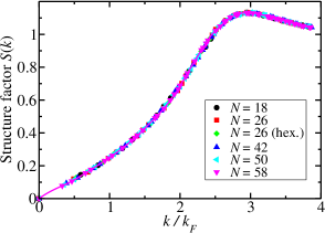
Figure 7: (Color online) VMC structure factor of the paramagnetic fluid at $D=0.63$ a.u. for a range of system sizes $N$.

VMC-calculated structure factors for paramagnetic and ferromagnetic hard-core gases are shown in Figs. 8 and 9, respectively. Finite-size “noise” is much worse for ferromagnetic phases. The fluid and crystal structure factors are similar, especially at low densities.

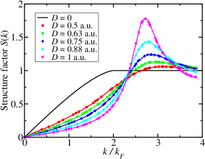
Figure 8: (Color online) VMC structure factors of paramagnetic fluids. For $D=0$ the analytic result for a paramagnetic free-particle gas is given.

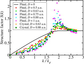
Figure 9: (Color online) VMC structure factors of ferromagnetic fluids and crystals. The $D=0$ result is the analytic structure factor for a ferromagnetic free-particle gas.

VI.3 Momentum density

VI.3.1 Results for fluids

The momentum density shown in Fig. 10 is reasonably well converged with respect to $N$. VMC results for the momentum densities of paramagnetic and ferromagnetic hard-core systems are shown in Figs. 11 and 12, respectively.

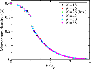
Figure 10: (Color online) VMC momentum density of the paramagnetic fluid at $D=0.88$ a.u. at different system sizes $N$.

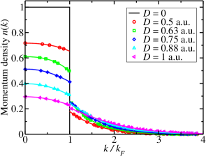
Figure 11: (Color online) VMC momentum densities of paramagnetic fluids at different hard-core diameters $D$.

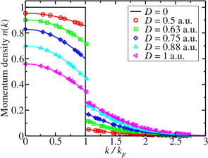
Figure 12: (Color online) VMC momentum densities of ferromagnetic fluids at different hard-core diameters $D$.

VI.3.2 Renormalization factors

The renormalization factor—the discontinuity $Z$ in the momentum density at the Fermi edge—is plotted against hard-core diameter in Fig. 13. The finite-size errors in $Z$ are oscillatory, so we have averaged over the results obtained for different system sizes $N$.

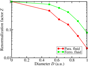
Figure 13: (Color online) Renormalization factor $Z$ against $D$, from fits to the momentum density.

VI.3.3 Results for crystals

The momentum densities of ferromagnetic hard-core crystals are shown in Fig. 14. This figure strongly confirms the conclusion that the crystal is unstable at $D=0.63$ a.u.: the “crystal” momentum density develops a near-discontinuity at the Fermi wave vector.

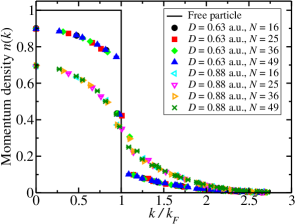
Figure 14: (Color online) VMC momentum densities of ferromagnetic crystals.

VII Weak, long-range interactions

VII.1 Form of the interaction

Our results show that, close to the transition from fluid to crystal, the energies of the paramagnetic and ferromagnetic fluids are very finely balanced, albeit with the paramagnetic fluid always lying lower in energy. It is interesting to ask whether a small change in the two-body potential might alter the relative stabilities of these two fluid phases and allow a region of stable ferromagnetic fluid.

As explained in Sec. I, it can be arranged that fermionic molecules confined to a plane experience an additional long-range, pairwise interaction varying as $\Lambda r^{-3}$, where $r$ is the interparticle separation and $\Lambda$ is a constant.innsbruck ; cooper_2009 In a finite, periodic cell, the two-body interaction between one particle and all the images of another particle that is at a distance ${\bf r}$ from the first is

$$v_{A}({\bf r}) = \sum_{\bf R}\frac{\Lambda}{|{\bf r}+{\bf R}|^{3}}$$

$$\approx \sum_{{\bf R}\in S}\frac{\Lambda}{|\tilde{{\bf r}}+{\bf R}|^{3}}+\frac{\Lambda}{A}\int_{R>R_{S}}\frac{d{\bf R}}{|\tilde{{\bf r}}+{\bf R}|^{3}}$$

$$\approx \sum_{{\bf R}\in S}\frac{\Lambda}{|\tilde{{\bf r}}+{\bf R}|^{3}}+\frac{2\pi\Lambda}{AR_{S}}\left(1+\frac{3\tilde{r}^{2}}{4R_{S}^{2}}\right)+O(R_{S}^{-5}),$$

where $S$ is a circular region of radius $R_{S}$ centered on the origin, and $\tilde{\bf r}$ is the minimum image of ${\bf r}$. By making $R_{S}$ sufficiently large, the approximation to the infinite sum can be made arbitrarily good.

The “Madelung” term (the interaction of each particle with its own images) is

$$v_{M} = \sum_{{\bf R}\neq{\bf 0}}\frac{\Lambda}{|{\bf R}|^{3}}$$ (14)

$$\approx \sum_{{\bf R}\in S-\{{\bf 0}\}}\frac{\Lambda}{|{\bf R}|^{3}}+\frac{\Lambda}{A}\int_{R>R_{S}}\frac{d{\bf R}}{|{\bf R}|^{3}}$$

$$\approx \sum_{{\bf R}\in S-\{{\bf 0}\}}\frac{\Lambda}{|{\bf R}|^{3}}+\frac{2\pi\Lambda}{AR_{S}}.$$

The Hamiltonian for the finite, periodic cell is therefore

$$\hat{H}=-\frac{1}{2}\sum_{i}\nabla_{i}^{2}+\sum_{i>j}\left[v_{H}(|\tilde{\bf r}_{ij}|)+v_{A}(\tilde{\bf r}_{ij})\right]+\frac{Nv_{M}}{2}.$$ (15)

VII.2 Convergence of the real-space sum

We have chosen $R_{S}$ such that 119 stars of lattice vectors are summed over explicitly in square cells (for fluid phases) and 86 stars are summed over in hexagonal cells (for crystal phases). The error in the Madelung constant is about $2\times 10^{-7}$ a.u. per particle for $N=18$ particles (and smaller at larger $N$). The error in the additional interaction per particle due to the finite number of stars of ${\bf R}$ vectors should therefore be much smaller than $10^{-6}$ a.u. The error made in truncating the real-space sum is therefore negligibly small compared with the statistical error bars on our QMC energies.

VII.3 Validity of perturbation theory

To a very good approximation we can describe the effect of the $\Lambda r^{-3}$ interaction using perturbation theory. The change in the energy resulting from the additional interaction is approximately given by the expectation of the interaction operator with respect to the previously optimized wave function for the unperturbed system, which can be evaluated using VMC. For $-1<\Lambda<1$, this approximation reproduces the full DMC energy difference to within about 0.002 a.u. at $D=0.88$ a.u., as shown in Fig. 15.

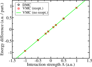
Figure 15: (Color online) Change in energy resulting from the inclusion of a $\Lambda r^{-3}$ interaction for a paramagnetic fluid of $N=18$ hard-core particles of diameter $D=0.88$ a.u.

VII.4 Finite-size errors

As with total energies, finite-size errors in the expectation value of the extra interaction are larger and quasi-random for the unstable phases. We extrapolate to infinite system size in each case, as shown in Fig. 16.

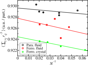
Figure 16: (Color online) VMC-evaluated expectation value of $\sum_{i>j}r_{ij}^{-3}$ with respect to the non-reoptimized VMC wave function.

VII.5 Effect of weak interactions on the phase diagram

At $D=0.88$ a.u., combining the VMC results for $\langle\sum_{i>j}r_{ij}^{-3}\rangle$ with the DMC energies in the absence of the additional interaction, we find that

$$E_{\rm PF} = 3.2559+0.9296\Lambda$$

$$E_{\rm FF} = 3.251+0.928\Lambda$$

$$E_{\rm FC} = 3.2305+0.9244\Lambda,$$ (16)

where $E_{\rm PF}$, $E_{\rm FF}$, and $E_{\rm FC}$ are the energies in a.u. per particle for the paramagnetic fluid, ferromagnetic fluid, and ferromagnetic crystals, respectively, as a function of $\Lambda$. The resulting offset in the energy relative to the energy of the paramagnetic fluid phase at a density close to the crystallization density is shown in Fig. 17. The changes in the energies of the three phases due to the inclusion of the $\Lambda r^{-3}$ tail are very similar. As one would expect, a repulsive potential ($\Lambda>0$) favors phases where the particles are kept apart (i.e., ferromagnetic over paramagnetic phases, and crystals over fluids), whereas an attractive interaction ($\Lambda<0$) favors a paramagnetic fluid the most and a ferromagnetic crystal the least. There is no region of stability for the ferromagnetic fluid, although it comes close at $\Lambda\approx-5$. However, this is a regime where the interaction is strongly attractive, so that perturbation theory is no longer valid, and a trial wave function that includes the possibility of superfluid pairing is required for accurate QMC calculations. It therefore seems unlikely that a weak interaction will have much effect on the phase diagram.

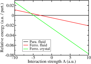
Figure 17: (Color online) Energy of the ferromagnetic fluid and crystal relative to the energy of the paramagnetic fluid against the strength of the $r^{-3}$ interaction for hard-core particles of diameter $D=0.88$ a.u.

VIII Conclusions

Gases of hard-core particles are a natural model for ultracold-atom systems. Correlation effects in 2D hard-core systems are surprisingly long-ranged. Our QMC results show that there is no regime in which itinerant ferromagnetism occurs in a 2D hard-core fluid. As the hard-core diameter $D$ is increased, the system undergoes a transition from a paramagnetic fluid to a crystal at $D=0.83$ a.u. The absence of a region of stability for a ferromagnetic fluid resembles the situation in the 2D HEG.ndd_2d_heg Including a weak $r^{-3}$ tail in the two-body interaction between hard-core particles does not lead to a significant revision of the phase diagram. We have presented QMC results for the PCFs, static structure factors, and momentum densities of the fluid phases of the hard-core gas.

- (1) I. Bloch, J. Dalibard, and W. Zwerger, Rev. Mod. Phys. 80, 885 (2008).
- (2) S. Giorgini, L. P. Pitaevskii, and S. Stringari, Rev. Mod. Phys. 80, 1215 (2008).
- (3) C. Chin, R. Grimm, P. Julienne, and E. Tiesinga, Rev. Mod. Phys. 82, 1225 (2010).
- (4) D. J. Papoular, G. V. Shlyapnikov, and J. Dalibard, Phys. Rev. A 81, 041603, (2010).
- (5) A. Micheli, G. Pupillo, H. P. Büchler, and P. Zoller, Phys. Rev. A 76, 043604 (2007).
- (6) A. V. Gorshkov, P. Rabl, G. Pupillo, A. Micheli, P. Zoller, M. D. Lukin, and H. P. Büchler, Phys. Rev. Lett. 101, 073201 (2008).
- (7) N. R. Cooper and G. V. Shlyapnikov, Phys. Rev. Lett. 103, 155302 (2009).
- (8) M. Greiner, O. Mandel, T. Esslinger, T. W. Hansch, I. Bloch, Nature 415,39 (2002).
- (9) R. A. Duine and A. H. MacDonald, Phys. Rev. Lett. 95, 230403 (2005).
- (10) G.-B. Jo, Y.-R. Lee, J.-H. Choi, C. A. Christensen, T. H. Kim, J. H. Thywissen, D. E. Pritchard, and W. Ketterle, Science 325, 1521 (2009).
- (11) D. Pekker, M. Babadi, R. Sensarma, N. Zinner, L. Pollet, M. W. Zwierlein, and E. Demler, arXiv:1005.2366 (2010).
- (12) M. Babadi, D. Pekker, R. Sensarma, A. Georges, and E. Demler, arXiv:0908.3483 (2009).
- (13) C. Nayak, S. H. Simon, A. Stern, M. Freedman, and S. Das Sarma, Rev. Mod. Phys. 80, 1083 (2008).
- (14) D. M. Ceperley and B. J. Alder, Phys. Rev. Lett. 45, 566 (1980).
- (15) W. M. C. Foulkes, L. Mitas, R. J. Needs, and G. Rajagopal, Rev. Mod. Phys. 73, 33 (2001).
- (16) J. B. Anderson, J. Chem. Phys. 65, 4121 (1976).
- (17) K. S. Liu, M. H. Kalos, and G. V. Chester, J. Low Temp. Phys. 13, 227 (1973).
- (18) C. De Michelis, G. Masserini, and L. Reatto, Phys. Rev. A 18, 296 (1978).
- (19) L. Xing, Phys. Rev. B 42, 8426 (1990).
- (20) S.-Y. Chang, M. Randeria, and N. Trivedi, Proc. Natl. Acad. Sci. USA 108, 51 (2011).
- (21) S. Pilati, G. Bertaina, S. Giorgini, and M. Troyer, Phys. Rev. Lett. 105, 030405 (2010).
- (22) R. J. Needs, M. D. Towler, N. D. Drummond, and P. López Ríos, J. Phys.: Condens. Matter 22, 023201 (2010).
- (23) N. D. Drummond, M. D. Towler, and R. J. Needs, Phys. Rev. B 70, 235119 (2004).
- (24) R. J. Needs, M. D. Towler, N. D. Drummond, and P. López Ríos, CASINO version 2.1 User Manual, University of Cambridge, Cambridge (2008).
- (25) P. López Ríos, A. Ma, N. D. Drummond, M. D. Towler, and R. J. Needs, Phys. Rev. E 74, 066701 (2006).
- (26) C. Lin, F. H. Zong, and D. M. Ceperley, Phys. Rev. E 64, 016702 (2001).
- (27) F. H. Zong, C. Lin, and D. M. Ceperley, Phys. Rev. E 66, 036703 (2002).
- (28) N. D. Drummond, Z. Radnai, J. R. Trail, M. D. Towler, and R. J. Needs, Phys. Rev. B 69, 085116 (2004).
- (29) B. Tanatar and D. M. Ceperley, Phys. Rev. B 39, 5005 (1989).
- (30) F. Rapisarda and G. Senatore, Aust. J. Phys. 49, 161 (1996).
- (31) N. D. Drummond and R. J. Needs, Phys. Rev. Lett. 102, 126402 (2009).
- (32) M. Li, H. Fu, Y.-Z. Wang, J. Chen, L. Chen, and C. Chen, Phys. Rev. A 66, 015601 (2002).
- (33) T. Kato, Commun. Pure Appl. Math. 10, 151 (1957); R. T. Pack and W. B. Brown, J. Chem. Phys. 45, 556 (1966).
- (34) C. J. Umrigar, M. P. Nightingale, and K. J. Runge, J. Chem. Phys. 99, 2865 (1993).
- (35) N. D. Drummond and R. J. Needs, Phys. Rev. B 79, 085414 (2009).
- (36) S. Chiesa, D. M. Ceperley, R. M. Martin, and M. Holzmann, Phys. Rev. Lett. 97, 076404 (2006).
- (37) N. D. Drummond, R. J. Needs, A. Sorouri, and W. M. C. Foulkes, Phys. Rev. B 78, 125106 (2008).
- (38) H. Akima, J. Assoc. Comput. Math. 17, 589 (1970).