Four-terminal resistance of an interacting quantum wire with weakly invasive contacts

Abstract

We analyze the behavior of the four-terminal resistance, relative to the two-terminal resistance of an interacting quantum wire with an impurity, taking into account the invasiveness of the voltage probes. We consider a one-dimensional Luttinger model of spinless fermions for the wire. We treat the coupling to the voltage probes perturbatively, within the framework of non-equilibrium Green function techniques. Our investigation unveils the combined effect of impurities, electron-electron interactions and invasiveness of the probes on the possible occurrence of negative resistance.

I Introduction

Quantum transport in novel materials, is one of the most active areas of present research in condensed matter physics QT . The problems that arise are specially interesting in one-dimensional (1D) devices such as quantum wires and carbon nanotubes. In these cases the effect of electron-electron (e-e) interactions is crucial, leading to the so called Luttinger liquid (LL) behavior 1D , characterized by correlation functions which decay with interaction-dependent exponents Exp-exponents and a power law in the tunneling $I-V$ characteristic curve powlawcond .

The actual nature of the resistance in a mesoscopic device has been a central issue since the first milestones in the theory of quantum transport. Landauer proposed the famous setup to study quantum transport where a mesoscopic sample is placed between two reservoirs at different chemical potentials. cond Then, Büttiker condbut , in agreement with experiments exp-cond , showed the fundamental relation $G=nG_{0}$ for the two-terminal conductance of a non-interacting quantum wire, being $n$ the number of transverse channels and $G_{0}=e^{2}/h$ the universal conductance quantum. The remarkable consequence of this simple law is the fact that a purely non-interacting electronic system without any kind of inelastic scattering mechanism has a sizable resistance, which for a single channel device is as large as $G_{0}^{-1}\simeq 13k\Omega$. This resistive behavior is due to the coupling between the system and the reservoirs through which the driving voltage is applied. For this reason, this quantity is identified as the contact resistance of the ideal non-interacting setup. The mesoscopic community became then motivated towards the definition of an alternative physical concept to describe the resistive behavior of the sample, free from the effects of the contact resistance. In another pioneering work engqan , a gedanken setup was proposed in order to sense the local voltage and the temperature. The main idea is to consider the mesoscopic system locally coupled to voltage probes or thermometers, represented by means of particle reservoirs. The latter have chemical potentials or temperatures that satisfy the condition of local electrochemical or thermal equilibrium with the mesoscopic system, which implies that the chemical potentials and temperatures of these systems are adjusted in order to get a vanishing electronic and heat flows through the contacts to the central device. For the case of two voltage probes connected along the sample as in the sketch of Fig. 1, the voltage drop corresponding to the chemical potential difference $(\mu_{1}-\mu_{2})/e$, defines the four terminal resistance

$$R_{4t}=\frac{\mu_{1}-\mu_{2}}{eI},$$ (1)

where $I$ is the current flowing through the setup. This scheme to define the four terminal resistance was later implemented in the framework of scattering matrix theory for multiterminal setups but4pt in wires of non-interacting electrons with a single but89 ; grambu and many impurities. gop In Refs. but89, ; grambu, it is clarified that the inference of $R_{4t}$ from a calculation based in a two-terminal geometry and the original Landauer formulacond may not always be correct, which stresses the importance of considering a genuine four-terminal setup to properly evaluate this quantity.

Among other interesting features, for non-interacting systems, it was predicted that negative four terminal resistances are possible. but4pt ; but89 ; grambu ; gop ; pern This is a consequence of the coherent nature of the electronic propagation along a sample where only elastic scattering processes with barriers or impurities can take place. These negative (longitudinal) resistances in ballistic structures were first measured in the late eighties takagaki-etal . More recently, this effect was also observed in semiconducting structures pic . A bit later, the behavior of $R_{4t}$ was experimentally studied in carbon nanotubes gao . In this case, a negative value of this resistance was also observed within the low temperature regime. Let us mention that the four-terminal resistance, in the context of uncorrelated fermions, has been also extended to the case of time-dependent voltage probes, leading to the concept of four-terminal impedance fed . It is widely accepted that the Luttinger model of interacting electrons in 1D is able to capture the main features observed in the transport experiments of carbon nanotubes lutran ; dolc . In particular, the power law behavior of the tunneling current as a function of the applied voltage and/or temperature predicted from Luttinger liquid theory has been experimentally observed in these systems. Regarding the behavior of $R_{4t}$ evaluated from a multiterminal setup in Luttinger liquids, the literature is restricted to Ref. ANS, . Previous estimates for this quantity were done on the basis of an interpretation of Landauer formula in a two terminal setup. egger This is due to the fact that quantum transport in multiterminals Luttinger liquids or models of interacting electrons is, in general, a rather challenging problem from the technical point of view. Besides Ref. ANS, , genuine multiterminal systems have been considered in Y-type geometries chamon ; lao , within linear response in the voltage and Hartree-Fock approximation of the interaction, respectively as well as in the study of the tunneling current of a quantum wire in the Fabry-Perot regime. pug There are also some recent works on the effect of wires that are capacitively coupled to an additional reservoir. caz ; zor

In Ref. ANS, we have considered the setup of Fig. 1, where an infinite Luttinger wire with a single impurity, through which a current $I$ flows as a response to an applied voltage $V$, is connected at two points to voltage probes. Following the procedure of previous works for non-interacting electrons, we have considered engqan ; but89 ; grambu ; gop ; pern non-invasive contacts between the wire and the voltage probes. We have shown that the voltage profile displays Friedel-like oscillations, as in the case of non-interacting electrons but89 ; pern ; grambu , but modulated by an envelope displaying a power law behavior as a function of the applied voltage or temperature, with an exponent depending on the electron-electron interaction strength. However, it is known that in the opposite limit of strong enough coupling between the mesoscopic device and the probes, inelastic scattering events and classical resistive behavior take place dampast . Moreover, ideal non-invasive probes cannot be easily realized in experimental situations. For this reason, the aim of the present study is to go a step beyond the assumption of non-invasive probes by considering probes that, while still weakly coupled to the sample, introduce decoherence through inelastic scattering processes, as well as inter-probe interference effects. Among other interesting questions, our goal is to answer if features in the behavior of the four-terminal resistance determined by non-invasive probes, like Friedel oscillations, or a negative value of this quantity, are still possible when the coupling of the probes becomes invasive. We address these issues in the framework of non-equilibrium Green functions and a perturbative treatment in the coupling to the probes.

The work is organized as follows. In section II, we present the model and the theoretical treatment to evaluate $R_{4t}$. In Section III and IV, we present results for the clean wire, and the wire with an impurity, respectively. Finally, we present a summary and conclusions in Section V. Some technical details are presented in an Appendix.

II Theoretical treatment

II.1 Model

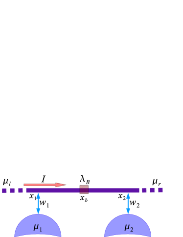
Figure 1: (Color online) Sketch of the setup: A voltage $V$ is imposed on a Luttinger liquid, through the chemical potentials for the left and right movers: $\mu_{r,l}=\mu\pm V/2$. Two voltage probes are connected at the positions $x_{1},x_{2}$. The corresponding chemical potentials $\mu_{1,2}$ are fixed by the condition of zero current through the contacts. An impurity is located at $x_{b}$.

We consider the setup of Fig.1. As in Ref. ANS, , we use the following action to describe the full system:

$$S=S_{wire}+S_{imp}+S_{res}+S_{cont}$$ (2)

where $S_{wire}$ corresponds to an infinite-length Luttinger wire and reads

$$S_{wire}=\int\,dx\,dt\,\Big{\{}\psi^{\dagger}_{l}\Big{[}i(\partial_{t}-\partial_{x})-\mu_{l}\Big{]}\psi_{l}+\psi^{\dagger}_{r}\Big{[}i(\partial_{t}+\partial_{x})-\mu_{r}\Big{]}\psi_{r}-g\left[\psi^{\dagger}_{r}\psi_{r}+\psi^{\dagger}_{l}\psi_{l}\right]^{2}\Big{\}},$$ (3)

with the first two terms corresponding to free spinless left and right movers respectively and $g$ is the e-e interaction in the forward channel. We use units where $\hbar=k_{B}=1$. We also take the Fermi velocity of the electrons $v_{F}=1$ and the electronic charge $e=1$. The two chemical potentials $\mu_{l}=\mu-V/2$ and $\mu_{r}=\mu+V/2$, for the left and right species, respectively, represent a voltage bias $V$ between the left and right ends of the wire, which generates a current $I$.

The effect of the impurity is described by a backward scattering term with strength $\lambda_{B}$ at a given position $x_{b}$:

$$S_{imp}=\lambda_{B}\int\,dx\,dt\,\delta(x-x_{b})\left[e^{-2ik_{F}x}\psi_{r}^{\dagger}\psi_{l}+\text{h.c.}\right].$$ (4)

We describe the voltage probes by $S_{res}$, corresponding to non-interacting electrons with two chiralities

$$S_{res} = \sum_{j=1,2}\int\,dy_{j}\,dt\,\Big{\{}\chi^{\dagger}_{l_{j}}\Big{[}i(\partial_{t}-\partial_{y_{j}})-\mu_{j}\Big{]}\chi_{l_{j}}$$ (5)

$$+\chi^{\dagger}_{r_{j}}\Big{[}i(\partial_{t}+\partial_{y_{j}})-\mu_{j}\Big{]}\chi_{r_{j}}\Big{\}},$$

The term $S_{cont}$ represents the tunneling between the reservoirs and the wire,

$$S_{cont} = \sum_{\begin{subarray}{c}j=1,2\\ \alpha=r,l,\beta_{j}=r_{j},l_{j}\end{subarray}}\int\,dx\,dy_{j}\,w_{j}\delta(x-x_{j})\delta(y_{j}-y_{j}^{0})$$ (6)

$$\times\left[e^{\mp i(k_{F}x+k_{F}^{(j)}y_{j})}\psi^{\dagger}_{\alpha}\chi_{\beta_{j}}+\text{h.c.}\right]$$

The upper and lower sign corresponds to $l$ and $r$, respectively, while $k_{F}$ and $k_{F}^{(j)}$ are the Fermi vectors of the wire and reservoirs, respectively. Note that here we are assuming that the voltage probes couple symmetrically to the left and right movers in the LL. This is a natural assumption in the absence of magnetic fields and spin-orbit interactions (Recall that we are considering a spinless LL). Since our main interest is to discuss the effects originated in the strength of the couplings, later, in Sections III and IV, as a simplifying hypothesis, we will consider the same coupling for both probes ($w_{1}=w_{2}$), although it is known that an asymmetrical coupling ($w_{1}\neq w_{2}$) is sufficient to produce a negative resistancetakagaki-etal ; ANS .

The tunneling current from the probes to the wire is

$$I_{j}=2\sum_{\alpha,\beta_{j}}\mbox{Re}\left[w_{j}G_{\alpha\beta_{j}}^{<}(x_{j},y_{j}^{0};t,t)\right],$$ (7)

where

$$G_{\alpha\beta_{j}}^{<}(x,y_{j};t,t^{\prime})=i<\chi_{\beta_{j}}^{\dagger}(y_{j},t^{\prime})\psi_{\alpha}(x,t)>,$$ (8)

is the lesser Green function involving degrees of freedom of the wire and reservoirs.

II.2 Green functions

In addition to the lesser Green function defined in Eq. (8), we define the following retarded Green functions:

$$G_{\alpha\beta}^{R}(x,x^{\prime};t,t^{\prime})=-i\Theta(t-t^{\prime})\langle\left\{\psi_{\alpha}(x,t),\psi^{\dagger}_{\beta}(x^{\prime},t^{\prime})\right\}\rangle$$

$$G_{\alpha\beta j}^{R}(x,x^{\prime};t,t^{\prime})=-i\Theta(t-t^{\prime})\langle\left\{\psi_{\alpha}(x,t),\chi^{\dagger}_{\beta j}(x^{\prime},t^{\prime})\right\}\rangle,$$ (9)

where the first one corresponds to degrees of freedom of the wire, while the second one corresponds to degrees of freedom of the wire and the $j$-th reservoir.

The evaluation of these Green functions implies the solution of the Dyson equations. For the sake of simplicity in the notation, it is convenient to carry out the following gauge transformations $\psi^{\dagger}_{l,r}(x)\rightarrow\psi^{\dagger}_{l,r}(x)e^{\pm ik_{F}x}$, $\chi^{\dagger}_{l_{j},r_{j}}(y_{j})\rightarrow e^{\pm ik_{F}^{(j)}y_{j}}\chi^{\dagger}_{l_{j},r_{j}}(y_{j})$. The Dyson equation for the retarded function reads

$$\{-i\partial_{t^{\prime}}\pm k_{F}-\mu_{\beta}\pm i\partial_{x^{\prime}}\}G_{\alpha\beta}^{R}(x,x^{\prime};t,t^{\prime})-\lambda_{B}G_{\alpha\overline{\beta}}^{R}(x,x^{\prime};t,t^{\prime})\delta(x^{\prime}-x_{b})=\delta(t-t^{\prime})\delta_{\alpha\beta}+$$

$$\sum_{j}w_{j}G_{\alpha\beta_{j}}^{R}(x,y_{j}^{0};t,t^{\prime})\delta(x^{\prime}-x_{j})+\sum_{\gamma}\int dx^{\prime\prime}dt^{\prime\prime}G_{\alpha\gamma}^{R}(x,x^{\prime\prime};t,t^{\prime\prime})\Sigma_{\gamma\beta}^{int}(x^{\prime\prime},x^{\prime};t^{\prime\prime},t^{\prime})$$ (10)

$$\{-i\partial_{t^{\prime}}\pm k_{F}^{(j)}\pm i\partial_{y_{j}}\}G_{\alpha\beta_{j}}^{R}(x,y_{j};t,t^{\prime})=w_{j}\sum_{\beta}G_{\alpha\beta}^{R}(x,x_{j};t,t^{\prime})\delta(y_{j}-y_{j}^{0}),$$ (11)

where the upper and lower signs correspond to $\beta=l,r$ and $\beta_{j}=l_{j},r_{j}$, respectively, and $\overline{l}=r$, $\overline{r}=l$, while $\Sigma_{\gamma\beta}^{int}(x^{\prime\prime},x^{\prime};t^{\prime\prime},t^{\prime})$ is the exact self-energy due to the interaction term with coupling constant $g$.

Let us now notice that the operator

$$-i\partial_{t^{\prime}}\pm k_{F}\pm i\partial_{y_{j}^{\prime}}=\left\{g_{\beta_{j}}^{R}(y_{j},y_{j}^{\prime};t,t^{\prime})\right\}^{-1},$$ (12)

is the inverse of the retarded Green function corresponding to the degrees of freedom $\beta_{j}$ of the reservoir $j$. Thus, Eq. (11) can be expressed as follows

$$G_{\alpha\beta_{j}}^{R}(x,y_{j}^{0};t,t^{\prime}) = w_{j}\sum_{\beta}\int dt^{\prime\prime}G_{\alpha\beta}^{R}(x,x_{j};t,t^{\prime\prime})$$ (13)

$$\times g_{\beta_{j}}^{R}(y_{j}^{0},y_{j}^{0};t^{\prime\prime},t^{\prime}).$$

Substituting the latter equation into Eq. (11) and defining

$$\Sigma_{\gamma\beta}^{res}(x,x^{\prime};t,t^{\prime}) = \sum_{j=1,2,\beta_{j}}\delta(x-x_{j})\delta(x^{\prime}-x_{j})|w_{j}|^{2}$$ (14)

$$\times g_{\beta_{j}}^{R}(y_{j}^{0},y_{j}^{0};t,t^{\prime}),$$

leads to

$$\{-i\partial_{t^{\prime}}\pm k_{F}-\mu_{\beta}\pm i\partial_{x^{\prime}}\}G_{\alpha\beta}^{R}(x,x^{\prime};t,t^{\prime})-\lambda_{B}G_{\alpha\overline{\beta}}^{R}(x,x^{\prime};t,t^{\prime})\delta(x^{\prime}-x_{b})=\delta(t-t^{\prime})\delta_{\alpha\beta}$$

$$+\sum_{\gamma}\int dx^{\prime\prime}dt^{\prime\prime}G_{\alpha\gamma}^{R}(x,x^{\prime\prime};t,t^{\prime\prime})\{\Sigma_{\gamma\beta}^{int}(x^{\prime\prime},x^{\prime};t^{\prime\prime},t^{\prime})+\Sigma_{\gamma\beta}^{res}(x^{\prime\prime},x^{\prime};t^{\prime\prime},t^{\prime})\}.$$ (15)

The lesser Green function entering the expression for the currents $I_{j}$ can be obtained by means of Langreth rules from (11) lang , according to which given $C^{R}(t,t^{\prime})=\int dt^{\prime\prime}A^{R}(t,t^{\prime\prime})B^{R}(t^{\prime\prime},t^{\prime})$ then $C^{<}(t,t^{\prime})=\int dt^{\prime\prime}[A^{R}(t,t^{\prime\prime})B^{<}(t^{\prime\prime},t^{\prime})+A^{<}(t,t^{\prime\prime})B^{A}(t^{\prime\prime},t^{\prime})]$, being the advanced function $[B^{A}]^{\dagger}=B^{R}$ . Thus

$$G_{\alpha\beta_{j}}^{<}(x_{j}^{0},y_{j}^{0};t,t^{\prime})=w_{j}\int dt^{\prime\prime}\left[G_{\alpha\alpha}^{<}(x_{j}^{0},x_{j}^{0};t,t^{\prime\prime})g_{\beta_{j}}^{A}(y_{j}^{0},y_{j}^{0};t^{\prime\prime},t^{\prime})+G_{\alpha\alpha}^{R}(x_{j}^{0},x_{j}^{0};t,t^{\prime\prime})g_{\beta_{j}}^{R}(y_{j}^{0},y_{j}^{0};t^{\prime\prime},t^{\prime})\right]$$ (16)

where $g^{A}=[g^{R}]^{\dagger}$ is the advanced Green function of the uncoupled reservoir.

So far all the equations are exact. The crucial step to obtain the exact Green function by solving Dyson equations is the evaluation of $\Sigma^{int}$, which corresponds to the fully dressed skeleton diagram for the self-energy corresponding to the electron-electron interaction, also taking into account the coupling to the two additional reservoirs as well as the backward impurity. We now introduce the following approximation for the limit of weak coupling to the reservoirs and the impurity such that $w_{j}\ll g$ and $\lambda_{B}\ll g$:

$$\Sigma_{\gamma\beta}^{int}(x,x^{\prime};t,t^{\prime})\simeq\Sigma_{\gamma\beta}^{Lutt}(x,x^{\prime};t,t^{\prime}),$$ (17)

where

$$\Sigma_{\gamma\beta}^{Lutt}(x,x^{\prime};t,t^{\prime})=[G^{R,Lutt}(x,x^{\prime};t,t^{\prime})]^{-1}_{\gamma\beta}-$$

$$\{-i\partial_{t^{\prime}}\pm k_{F}\pm i\partial_{x^{\prime}}\}\delta_{\gamma\beta},$$ (18)

is the self-energy of the infinite Luttinger wire without impurity and uncoupled from the reservoirs, while $G^{R,Lutt}(x,x^{\prime};t,t^{\prime})$ is the ensuing retarded Green function. The approximation (17) implies the evaluation of the self-energy associated to e-e interaction by neglecting vertex corrections due to the escape to the reservoirs and due to the scattering with the impurity. This approximation is adequate only in the limit of small $w_{j}$ and $\lambda_{B}$.

Under this approximation in the e-e self-energy and performing a Fourier transform with respect to $t-t^{\prime}$, Eq. (15) can be expressed as follows

$$G_{\alpha\beta}^{R}(x,x^{\prime};\omega)=G_{\alpha\beta}^{R,Lutt}(x,x^{\prime};\omega)+\sum_{j}G_{\alpha\alpha}^{R}(x,x_{j},\omega)\Sigma^{res}_{\alpha\beta}(x_{j},x_{j};\omega)G_{\beta\beta}^{R,Lutt}(x_{j},x^{\prime};\omega)+G_{\alpha\alpha}^{R}(x,x_{b},\omega)\lambda_{B}G_{\beta\beta}^{R,Lutt}(x_{b},x^{\prime};\omega)$$ (19)

This equation allows for the evaluation of the retarded Green function. In what follows, we solve it at the lowest order in the backscattering term $\lambda_{B}$ and up to ${\cal O}(w_{j}^{2})$, in the coupling to the voltage probes. We recall that ideal non-invasive probes correspond to keeping only up to ${\cal O}(w_{j})$. It is important to notice that in the limit of vanishing Coulomb interaction ($g=0$), the above equation leads the exact retarded Green function of the problem.

II.3 Currents

Substituting Eq. (16) in the definition of the current (7), we get the following exact equation for the current flowing through the contact between the $j$-th reservoir and the wire

$$I_{j}=-2\sum_{\alpha\beta,j}\mbox{Re}\left\{w_{j}^{2}\int\frac{d\omega}{2\pi}\left[G_{\alpha\alpha}^{<}(x_{j}^{0},x_{j}^{0};\omega)g_{\beta_{j}}^{A}(r_{j}^{0},r_{j}^{0};\omega)+G_{\alpha\alpha}^{R}(x_{j}^{0},x_{j}^{0};\omega)g_{\beta_{j}}^{<}(r_{j}^{0},r_{j}^{0};\omega)\right]\right\}.$$ (20)

Making use of the assumption of weak coupling between the probes and the wire and weak amplitude in the back scattering term induced by the impurity, we evaluate the Green functions $G_{\alpha\alpha}^{<}(x_{j}^{0},x_{j}^{0};\omega)$ and $G_{\alpha\alpha}^{R}(x_{j}^{0},x_{j}^{0};\omega)$ perturbatively up to ${\cal O}(w_{j}^{2})$ and ${\cal O}(\lambda_{B})$. Concretely, this implies solving (19) as

$$G_{\alpha\beta}^{R}(x,x^{\prime};\omega) \simeq G_{\alpha\beta}^{R,Lutt}(x,x^{\prime};\omega)+\sum_{j}G_{\alpha\alpha}^{R,Lutt}(x,x_{j},\omega)\Sigma^{res}_{\alpha\beta}(x_{j},x_{j};\omega)G_{\beta\beta}^{R,Lutt}(x_{j},x^{\prime};\omega)$$ (21)

$$+G_{\alpha\alpha}^{R,Lutt}(x,x_{b},\omega)\lambda_{B}G_{\beta\beta}^{R,Lutt}(x_{b},x^{\prime};\omega),$$

while the lesser counterpart can be derived from (21) by recourse to Langreth rules (see above Eq. (16)). The explicit expression for $G_{\alpha\alpha}^{R,Lutt}(x,x_{j},\omega)$ is given in Appendix A. After some algebra, the currents through the contacts can be expressed as follows

$$I_{j}=I^{(1)}_{j}+I^{(2)}_{j},$$ (22)

where $I^{(1)}_{j}\propto|w_{j}|^{2}$, $I^{(2)}_{j}\propto|w_{j}|^{4}$, being

$$I_{j}^{(1)} = 2w_{j}^{2}\sum_{\alpha=l,r}\int_{-\infty}^{\infty}\frac{d\omega}{2\pi}\Bigg{\{}G^{<,Lutt}_{\alpha\alpha}(x_{j},x_{j},\omega)g_{j}^{>}(\omega)-G^{>,Lutt}_{\alpha\alpha}(x_{j},x_{j},\omega)g_{j}^{<}(\omega)$$

$$+\lambda_{B}\Big{[}[G_{\alpha\alpha}^{<,Lutt}(x_{j}-x_{b};\omega)\left(G_{\overline{\alpha}\overline{\alpha}}^{R,Lutt}(x_{j}-x_{b};\omega)\right)^{\ast}+G_{\alpha\alpha}^{R,Lutt}(x_{j}-x_{b};\omega)G_{\overline{\alpha}\overline{\alpha}}^{<,Lutt}(x_{b}-x_{j})]g_{j}^{>}(\omega)-$$

$$- [G_{\alpha\alpha}^{>,Lutt}(x_{j}-x_{b};\omega)\left(G_{\overline{\alpha}\overline{\alpha}}^{R,Lutt}(x_{j}-x_{b};\omega)\right)^{\ast}+G_{\alpha\alpha}^{R,Lutt}(x_{j}-x_{b};\omega)G_{\overline{\alpha}\overline{\alpha}}^{>,Lutt}(x_{b}-x_{j})]g_{j}^{<}(\omega)\Big{]}\Bigg{\}}$$ (23)

$$I_{j}^{(2)} = 4w_{j}^{2}\sum_{\begin{subarray}{c}i=1,2\\ \alpha,\beta=r,l\end{subarray}}w_{i}^{2}\int_{\infty}^{\infty}\frac{d\omega}{2\pi}\Big{\{}G_{\alpha\alpha}^{R,Lutt}(x_{j},x_{i},\omega)G_{\beta\beta}^{A,Lutt}(x_{i},x_{j},\omega)\left[g_{j}^{>}(\omega)g_{i}^{<}(\omega)-g_{j}^{<}(\omega)g_{i}^{>}(\omega)\right]+$$

$$+ G_{\alpha\alpha}^{R,Lutt}(x_{j},x_{i},\omega)g_{i}^{R}(\omega)\left[G^{<,Lutt}_{\beta\beta}(x_{i},x_{j},\omega)g_{j}^{>}(\omega)-G^{>,Lutt}_{\beta\beta}(x_{i},x_{j},\omega)g_{j}^{<}(\omega)\right]+$$

$$+ G_{\alpha\alpha}^{A,Lutt}(x_{i},x_{j},\omega)g_{i}^{A}(\omega)\left[G^{<,Lutt}_{\beta\beta}(x_{j},x_{i},\omega)g_{j}^{>}(\omega)-G^{>,Lutt}_{\beta\beta}(x_{j},x_{i},\omega)g_{j}^{<}(\omega)\right]\Big{\}}$$

The term $I^{(1)}_{j}$ corresponds to the limit of ideal non-invasive contacts considered in Ref. ANS, . It is derived by dropping the second term in Eq. (21) and the ensuing term in the lesser counterpart. This leads to the exact solution ${\cal O}(w_{j})$ of (15) and (16) for $\lambda_{B}=0$. In the second-order solutions (21) we have introduced the additional approximation of neglecting vertex corrections $\propto w_{j}^{2}$ and $\propto\lambda_{B}$ in the evaluation of the many-body self-energy $\Sigma^{int}$. Notice that the two probes are completely uncorrelated within the ”non-invasive” component $I^{(1)}$. In the higher order contribution $I^{(2)}$ it is possible to distinguish two kinds of terms. On one hand, those $\propto w_{j}^{4}$, account for the effect of dephasing and resistive behavior induced by the inelastic scattering processes due to the coupling to the reservoirs. On the other hand, terms $\propto w_{1}^{2}w_{2}^{2}$ describe interference effects between the two probes.

It is now convenient to express the lesser and greater Green function in terms of spectral functions:

$$G_{\alpha,\alpha}^{<,>,Lutt}(x_{1}-x_{2};\omega+\mu_{\alpha}) = \lambda^{<,>}_{\alpha}(\omega)\rho_{\alpha}(x_{1}-x_{2};\omega),$$

$$g_{j}^{<,>}(\omega) = \lambda^{<,>}_{j}(\omega)\rho_{j}(\omega)$$ (25)

with $\lambda^{<}_{\alpha,j}(\omega)=in_{F,\alpha,j}(\omega)$, $\lambda^{>}_{\alpha,j}(\omega)=-i[1-n_{F,\alpha,j}(\omega)]$, being $n_{F,\alpha}(\omega)=1/(e^{(\omega\pm V/2)/T}+1)$, the Fermi function where the upper and lower signs corresponds, respectively to the right and left movers of the wire, and $n_{F,j}(\omega)=1/(e^{(\omega-\mu_{j})/T}+1)$, $\mu_{j}$ being the chemical potentials of the electrons in the $j$ reservoir, relative to the mean chemical potential $\mu$ of the wire. $T$ is the temperature, which we assume to be the same for the wire and the probes, while $\rho_{\alpha}(\omega)=iG^{R,Lutt}_{\alpha\alpha}(x_{1}-x_{2};\omega)-i[G^{R,Lutt}_{\alpha\alpha}(x_{2}-x_{1};\omega)]^{*}$ is the spectral function for the $\alpha$ movers in the Luttinger model, and $\rho_{j}(\omega)=-2\mbox{Im}[g^{R}_{j}(\omega)]$, is the spectral density of the $j$ probe. Replacing in (II.3) and (II.3), the full expression for the current reads:

$$I_{j} = 2w_{j}^{2}\sum_{\alpha,\beta=l,r}\int_{\infty}^{\infty}\frac{d\omega}{2\pi}[n_{F,\alpha}(\omega)-n_{F,j}(\omega)]\rho_{j}(\omega)\{\rho_{\alpha}(0,\omega)\left[1+2w_{j}^{2}\mbox{Re}\left(G_{\beta}^{R,Lutt}(0,\omega)g_{j}^{R}(\omega)\right)\right]+$$ (26)

$$+2\lambda_{B}\mbox{Re}\left[\rho_{\alpha}(x_{j}-x_{b};\omega)\left(G_{\bar{\alpha}}^{R,Lutt}(x_{j}-x_{b};\omega)\right)^{\ast}\right]+\qquad 2w_{\bar{j}}^{2}\mbox{Re}\left[\rho_{\alpha}(x_{j}-x_{\bar{j}};\omega)^{\ast}G_{\beta}^{R,Lutt}(x_{j}-x_{\bar{j}};\omega)g_{\bar{j}}^{R}(\omega)\right]\}$$

$$+2w_{j}^{2}w_{\bar{j}}^{2}\sum_{\alpha,\beta=l,r}\int_{\infty}^{\infty}\frac{d\omega}{2\pi}\left[n_{F}(\omega-\mu_{\bar{j}})-n_{F}(\omega-\mu_{j})\right]\rho_{j}(\omega)\rho_{\bar{j}}(\omega)G_{\beta}^{R,Lutt}(x_{j}-x_{\bar{j}};\omega)\left(G_{\alpha}^{R,Lutt}(x_{j}-x_{\bar{j}};\omega)\right)^{\ast},$$

where we use the notation $j,\bar{j}$ such that $\bar{1}=2$ and $\bar{2}=1$.

II.4 Voltage drop and four-terminal resistance

The chemical potentials $\mu_{j}$ in the expressions of the previous subsection must be set to satisfy the condition of local electrochemical equilibrium between the probes and the wire. This implies vanishing flows $I_{j}=0$, $j=1,2$, with the currents defined in Eq. (26), and the two chemical potentials $\mu_{j}$ must satisfy these constraints. In the case of non-invasive probes, the two probes are completely uncorrelated, and the problem can be reduced to that of the wire coupled to a single probe, which senses the local chemical potential of the wire. Instead, in the present case, we have to solve a system of two non-linear equations to calculate $\mu_{1}$ and $\mu_{2}$, from where the voltage drop $\Delta V=\mu_{1}-\mu_{2}$ between the points $x_{1}$ and $x_{2}$ of the wire coupled to the two probes can be evaluated. This voltage drop contains not only information of the scattering processes in the wire that are independent of the coupling to the probes, but also of inelastic scattering processes and interference effects introduced by the probes themselves. The four-terminal resistance can be evaluated from Eq. (1) and the ratio between the four-terminal and two terminal resistance $R_{2t}=V/I$ results

$$\frac{R_{4t}}{R_{2t}}=\frac{\Delta V}{V}.$$ (27)

The two chemical potentials are evaluated numerically from Eq. (26), with the Green functions given in Appendix A.

III Results without impurity

In this section we show results for the ratio between $R_{4t}/R_{2t}$ in the case of $\lambda_{B}=0$. It is important to mention that in the limit of non-invasive probes, this ratio vanishes identically under this case, and all the features in the behavior of the resistance discussed in this section are solely due to the invasive nature of the probes.

We characterize the strength of e-e interactions with the parameter $K=(1+\frac{2g}{\pi})^{-1/2}$. The limit of non-interacting electrons corresponds to $K=1$ while typical values of $K$ (experimentally determined in transport measures in nanodevices K-values ) are in the range $0.25<K<0.75$.

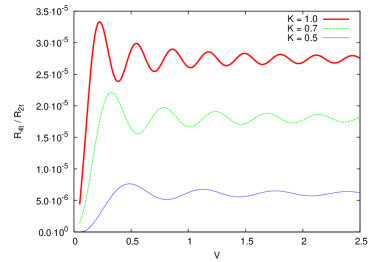
Figure 2: (Color online)$R_{4t}/R_{2t}$ as a function of the voltage $V$, for different values of the e-e interaction strength $K$. The positions of the probes are $x_{1}=-10$ and $x_{2}=10$, and the strength of the couplings are $w_{1}=w_{2}=0.1$. The temperature is $T=0$.

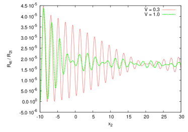
Figure 3: (Color online) $R_{4t}/R_{2t}$ as a function of the position of the second probe $x_{2}$, given the first probe fixed at $x_{1}=-10.$. The strength of the e-e interaction is $K=0.7$, and the couplings $w_{1}=w_{2}=0.1$.

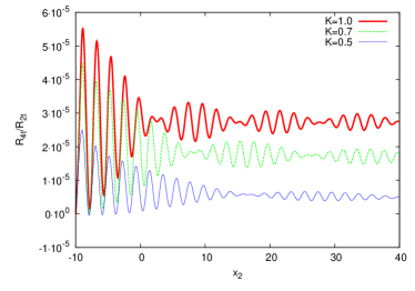
Figure 4: (Color online) $R_{4t}/R_{2t}$ as a function of the position of the second probe $x_{2}$, given the first probe fixed at $x_{1}=-10.$, for different values of the e-e interaction strength $K$. We set $T=0$, $w_{1}=w_{2}=0.1$ and $V=1$.

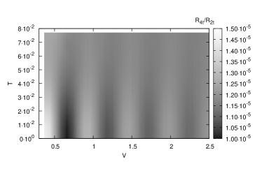
Figure 5: (Color online)$R_{4t}/R_{2t}$ as a function of the voltage $V$ and the temperature $T$, for $K=0.7$. The positions of the probes are $x_{1}=-10.$ end $x_{2}=10.$, and the strength of the couplings are $w_{1}=w_{2}=0.1$.

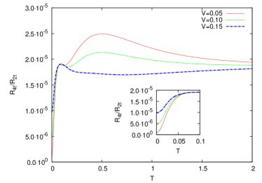
Figure 6: (Color online)$R_{4t}/R_{2t}$ as a function of the temperature $T$, for $K=0.7$ and three values of $V$. The positions of the probes are $x_{1}=-10.$ end $x_{2}=10.$, and the strength of the couplings are $w_{1}=w_{2}=0.1$. Inset: low temperature regime.

Results for $R_{4t}/R_{2t}$ as a function of the bias voltage $V$, for the probes connected at two fixed positions and different values of the e-e interaction $K$ are shown in Fig. 2 In order to gain insight on the behavior of the ratio between resistances, let us notice that for vanishing bias voltage $V$, the voltage drop $\Delta V$ and thus $R_{4t}/R_{2t}$ should be also vanishing. It is, therefore, not surprising that for low enough $V$, $R_{4t}/R_{2t}$ displays a power law behavior as a function of $V$,

$$\frac{R_{4t}}{R_{2t}}\propto V^{2\gamma+1}.$$ (28)

The exponent $\gamma$ is related to the Luttinger parameter as $\gamma=(K+K^{-1}-2)/4$. The latter result can be rather straightforwardly derived from an expansion of $I_{j}$ for low $V$. On the other hand, a classical ohmic-like resistive behavior implies a constant value of $R_{4t}/R_{2t}$. In Fig. 2, it can be seen that such a behavior is approximately attained when the bias voltage overcomes a value $V_{c}$, which satisfies $eV_{c}\approx\hbar v/(2K\mid x_{1}-x_{2}\mid)$. note This energy scale can be understood by noticing that $v/K$ is the plasmon velocity along the wire and $\tau_{p}=2K\mid x_{1}-x_{2}\mid/v$ is the time that these excitations take for a round trip between the probes. The latter defines the characteristic time for the inelastic back-scattering processes. Notice, that although the Luttinger wire is an elastic system, where electrons propagate ballistically, the coupled voltage probes act as a dissipative bath. In fact, it is precisely the coupling to reservoirs the mechanism usually followed in the literature (see, for example Refs. dampast, and caz, ) in order to model Ohmic dissipation. In the present case, assuming that the bias is applied from left to right, the Fermi energy of right-moving electrons is an amount $eV$ higher than that of the left-moving ones. Then, the energy associated to the crossover voltage $eV_{c}$ corresponds to the energy dissipated in the contacts, in a process in which an electron with the Fermi energy $\mu_{R}$ travels with velocity $v/K$ from the left probe, connected at $x_{1}$, to the right one, connected at $x_{2}$, it is backscattered at $x_{2}$ and comes back to $x_{1}$ with a Fermi energy $\mu_{L}$. An estimate for the energy transfer involved in the dissipative process is, precisely, $\hbar\tau_{p}^{-1}$. The above argument can be easily reconstructed for the case of a bias with opposite sign, in which case, the energy is inelastically transferred from right to left movers. Notice that in any case, the energy dissipated at the contacts is associated to a voltage drop that has the same direction as the external bias, as is expected for a classical Ohmic-like process. Interestingly, $2\tau_{p}^{-1}$ is equivalent to the ballistic frequency defined in Ref. dolc, for an interacting Luttinger wire of finite length connected to reservoirs.

To summarize, for a given separation $\mid x_{1}-x_{2}\mid$ between the two probes, $V_{c}$ defines the crossover voltage for which inelastic back-scattering processes between the two points become active. Notice that the low voltage regime $V<V_{c}$ so defined, depends on the e-e interaction strength $g$, being wider for stronger $g$ (lower $K$). In general, the effect of this interaction is to decrease the resistance. A closer analysis of Fig. 2 for $V>V_{c}$ reveals that $R_{4t}/R_{2t}$ as a function of the bias voltage $V$ displays oscillatory features. This can be naturally interpreted as the consequence of interference effects between the two probes. From fits of the numerical data, we found that they can be very well reproduced by a function of the form:

$$\frac{R_{4t}}{R_{2t}}\approx A+B\sin(KV(x_{2}-x_{1}))/V^{2\gamma+1},\;\;\;\;V>V_{c},$$ (29)

with $A$ and $B$ depending on $K$ while proportional to $w^{2}$, although we have not derived this result analytically from Eq. (26). It is anyway interesting that a similar resistive behavior is obtained in a Luttinger wire of finite length in the presence of back-scattering processes (see Refs. dolc, ; pug, ). Another interesting observation is that the saturation value $A$ decreases for increasing electron-electron interactions, This indicates that the latter tend to screen the inelastic scattering processes introduced by the coupling to the probes.

In Fig. 3 we show the behavior of the ratio between resistances with the position of one of the probes kept fixed while the position of the second one is moved along the wire. This pattern reveals that the functional behavior is

$$\frac{R_{4t}}{R_{2t}}\approx A+B\sin(2k_{F}(x_{2}-x_{1}))\sin(KV(x_{2}-x_{1}))/V^{2\gamma+1},$$ (30)

within the high $V>V_{c}$ voltage regime, corresponding, respectively, to solid and dashed lines in the Figure. The $2k_{F}$ modulation resembles the behavior found in the voltage profile of non-invasive probes in a system with an impurity, which is observed both in non-interacting but89 ; pern ; grambu and interacting systems ANS . In those cases the origin is the occurrence of interference in the electronic wave packet generated by the back-scattering processes that take place at the impurity. In the present case, the interference is originated by scattering processes at the probes. Unlike the behavior for non-invasive probes, in our case the voltage drop induced by the probes has the same sign as the applied external voltage. This means that the four-terminal resistance for invasive probes in a clean wire is always positive, in spite of the Friedel-like $2k_{F}$ oscillations. This is in strong contrast to the case of non-invasive probes, where these oscillations provide a mechanism for $R_{4t}<0$. Fig. 4 illustrates the same situation but for fixed voltage and varying $K$. One sees that, in general, larger values of the e-e interactions produce smaller values of $R_{4t}/R_{2t}$. Then we conclude that, although one cannot have negative values of the four terminal resistance in the absence of impurities, e-e interactions tend to facilitate that possibility.

In Fig. 5 we show the effect of the temperature in the behavior of $R_{4t}/R_{2t}$. It is clear that, as the temperature increases, the oscillations discussed in Fig. 2 within the high voltage regime, tend to be wiped out and the resistance evolves to a constant value. This behavior is depicted in more detail in Fig. 6, where we display $R_{4t}/R_{2t}$ as function of $T$ for three different values of the bias voltage $V$. In analogy with the previously discussed behavior found at $T=0$, as function of $V$ (Fig.2), there is a crossover temperature $T_{c}\approx\hbar v/(2K\mid x_{1}-x_{2}\mid)$ which allows to distinguish low and high temperature regimes. For low temperatures ($T<T_{c}$), we have verified that the ratio between resistances behaves as

$$\frac{R_{4t}}{R_{2t}}\simeq a+b\,T^{2\gamma+1},$$ (31)

where $a$ and $b$ depend on $V$. For high temperatures $R_{4t}/R_{2t}$ tends to a constant value. As the temperature increases, coherence tends to disappear. For this reason, no signature of the oscillatory behavior observed in Fig. 2 is found here. The interplay between $T$ and $V$ gives rise to the possible occurrence of a global maximum of the $R_{4t}/R_{2t}$. The value of temperature that corresponds to this maximum, when it is present, depends on $K$ and $\mid x_{1}-x_{2}\mid$.

IV Results with impurity

In this section we analyze the behavior of $R_{4t}/R_{2t}$ at $T=0$, for a wire with an impurity with backscattering strength $\lambda_{B}$. In the case of non-invasive probes, the local voltage displays $2k_{F}$ Friedel-like oscillations with constant amplitude for non-interacting electrons but89 ; pern ; grambu , and with modulated amplitude in the case of and interacting wire. ANS

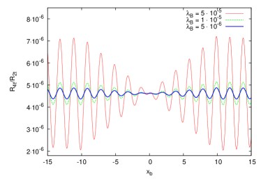
Figure 7: (Color online) $R_{4t}/R_{2t}$ as a function of the position of the impurity $x_{b}$, for probes connected at $x_{1}=-10.$ and $x_{2}=10$. The bias voltage is $V=0.5$, the strength of the e-e interaction is $K=0.7$, and the couplings $w_{1}=w_{2}=0.1$. Different plots correspond to different strengths of the backscattering term representing the impurity.

Figure 7 shows $R_{4t}/R_{2t}$ for the probes connected at fixed positions, as a function of the position of the impurity $x_{b}$. Friedel-like oscillations with period $2k_{F}$ are identified, with an increasing amplitude for increasing back-scattering strength. As in the case of non-invasive probes, the amplitude is modulated for interacting electrons, the local voltage achieving the highest amplitudes at the position of the impurity. Unlike the case of non-invasive probes, the oscillations take place with respect to a constant non-vanishing value, which is determined by the degree of coupling of the probes. For the parameters shown in the figure, $R_{4t}$ is always a positive quantity.

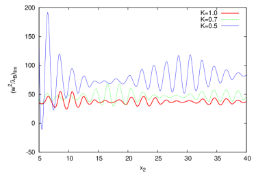
Figure 8: (Color online) The ratio $(w_{j}^{2}/\lambda_{B})_{lim}$ at which $R_{4t}=0$ for $x_{1}=x_{b}=-10$, as a function of the position of the second probe $x_{2}$. Different plots correspond to different e-e interaction parameters $K$. The applied voltage is $V=0.5$.

Besides interference effects, it is clear that the coupling of the probes generates classical resistive behavior through inelastic scattering processes, while the elastic scattering induced by the impurity induce Friedel oscillations. The first type of processes takes place with a strength $\propto w_{j}^{2}/\Lambda^{\prime}$, where $\Lambda^{\prime}$ is the bandwidth of the reservoirs, while the second one takes place with a strength $\lambda_{B}$. The two mechanisms are competitive regarding the possibility of having $R_{4t}<0$. In Fig. 8 we analyze, precisely, this possibility. To this end, we have fixed the first probe at the position $x_{1}=x_{b}=-10$, where the minimum $R_{4t}/R_{2t}$ is achieved, considering different positions for the second probe $x_{2}$. For each of these configurations we then vary the ratio $w_{j}^{2}/\lambda_{B}$, to define $(w_{j}^{2}/\lambda_{B})_{lim}$, at which $R_{4t}/R_{2t}=0$. The corresponding results are plotted in the figure for different e-e interactions. For $w_{j}^{2}/\lambda_{B}>(w_{j}^{2}/\lambda_{B})_{lim}$ the ratio $R_{4t}/R_{2t}$ is positive for any value of $x_{b}$. On the other hand, the condition $w_{j}^{2}/\lambda_{B}<(w_{j}^{2}/\lambda_{B})_{lim}$ defines the values of coupling strength for which a negative four terminal resistance is possible, depending on the position of the impurity.

A very interesting and subtle issue that is also revealed by our analysis concerns the role of e-e interactions in the possible occurrence of a negative four-terminal resistance. Based on the results obtained for non-invasive probes but89 ; pern ; grambu ; ANS one would expect that e-e interactions oppose to such possibility, owing to the fact that for stronger interactions (smaller values of $K$) the amplitude of the oscillations coming from the presence of the impurity diminishes. However, in the present case this effect competes with the global ”upward” shift coming from the contribution of $I^{(2)}_{j}$. In other words, as already pointed out in Section III, the weak invasiveness of the probes, which in our formulation is contained in $I^{(2)}_{j}$ produces a voltage drop that has the same sign of the bias $V$. It turns out that the magnitude of such a shift also depends on $K$, and it decreases for increasing interactions (decreasing $K$), as shown in Figures (2) and (6). The combination of these two effects gives rise to the result depicted in Fig.(8), where one sees that for sufficiently separated probes, e-e interactions facilitate the occurrence of a negative four-terminal resistance.

V Summary and Conclusions

We have analyzed the behavior of the four terminal resistance in a biased quantum wire with an impurity. We have modeled the wire by an infinite-length Luttinger wire where the bias voltage is represented by different chemical potentials for the left and right movers, and the impurity by a backscattering term. We have also introduced models for the probes, which consist in reservoirs of non-interacting electrons. These systems are locally weakly coupled to the wire and have chemical potentials satisfying the conditions of vanishing electronic currents between the reservoirs and the wire. The difference between the so determined chemical potentials defines the voltage drop, from where the ratio between the four-terminal and two-terminal resistance can be calculated. We have solved the problem within perturbation theory in the impurity strength and the tunneling parameter defining the coupling between the probes and the wire, within the framework of non-equilibrium Green functions formalism. We have neglected vertex corrections in the self-energy for the e-e interaction associated to inelastic scattering processes due to the escape to the leads and elastic scattering processes at the impurity. Since we have assumed that these two parameters are small enough, the latter is expected to be a reliable approximation.

We have analyzed the voltage drop beyond the non-invasive assumption for the coupling of the probes to the wire. That is, we have studied, not only the voltage drop originated by elastic scattering processes along the wire, but also the effects introduced by the coupling to the probes, itself. We have shown that the inelastic scattering processes due to the invasive coupling of the probes induce a voltage drop with a power law behavior as a function of the bias voltage for low values of this parameter, with an exponent determined by the e-e interaction. In the limit of non-interacting electrons, this reduces to a linear dependence as a function of the bias voltage. This behavior has classical and quantum features, since the voltage drop is always in the same sense of the applied voltage but displays a pattern of oscillations indicating quantum interference between the two probes. These features, are, however, screened as the e-e interaction increases. In our calculations, we have considered an infinite wire. However, the separation between the probes sets a natural length scale in the problem, which determines the crossover value of the bias voltage for which inelastic scattering processes become active. In the case of an interacting wire with finite length, we expect that our results remain valid provided the length of the wire is much larger than the separation between the probes. In the presence of an impurity, the elastic backward scattering processes and $2k_{F}$ oscillations detected by non-invasive probes ANS are superimposed to the inelastic processes introduced by the probes.

Our results have an important outcome in relation to experimental measurements of four-terminal resistance in real systems. That is, for invasive probes, elastic effects like those generated by backscattering processes by impurities can still lead to a voltage drop that opposes to the applied voltage, giving rise to a negative four-terminal resistance. However, the amplitude for these processes must be high enough in order to overcome the classical resistive effect introduced by the probes.

As far as the e-e interaction effects are concerned, they play a fundamental role in the calculated magnitudes. For higher e-e interaction, the oscillations amplitude coming from the impurity decreases. The amplitude of the global shift coming from the interaction of the probes also decreases for stronger interactions. We have shown that if the separation of the probes is large enough, the possibility of measuring a negative resistance increases for stronger interactions.

VI Acknowledgments

We acknowledge support from CONICET and ANPCYT, Argentina, as well as UBACYT and the J. S. Guggenheim Memorial Foundation (LA).

Appendix A Green functions and spectral functions for the Luttinger wire and the reservoirs

We can follow the procedure of Ref. gflut, to evaluate the retarded Green functions of the Luttinger wire and calculate the spectral density from $\rho_{\alpha}(x,x^{\prime};\omega)=i[G^{R,Lutt}_{\alpha}(x-x^{\prime};\omega)-G^{R,Lutt}_{\alpha}(x^{\prime}-x;\omega)^{*}]$. The result is

$$\rho_{\alpha}(x,x^{\prime};\omega+\mu_{\alpha}) = C\exp\left[\mp i\left(\frac{\omega}{v}-k_{F}\right)x\right]|\omega|^{2\gamma}$$ (32)

$$\times\phi(\gamma,2\gamma+1,\pm 2ix\omega/v),$$

where $\phi$ is Kummer’s Hypergeometric function, $\gamma=(K+K^{-1}-2)/4$ and $v=1/K$. In order to perform numerical calculations, we introduce an energy cutoff $\Lambda$ such that $\rho(x,\omega+\mu)\rightarrow\rho(x,\omega+\mu)\Theta(\Lambda-|\omega|)$. $C$ is a normalization constant, which can be evaluated by the normalization condition

$$\int\frac{d\omega}{2\pi}\rho(x,\omega)\big{|}_{x=0}=1$$ (33)

The retarded and advanced green function are then calculated using the Kramers-Kronig relations

$$G^{R,Lutt}(x,\omega) = \int\frac{d\omega^{\prime}}{2\pi}\frac{\rho(x,\omega^{\prime})}{\omega-\omega^{\prime}+i\eta}=$$ (34)

$$= \int\frac{d\omega^{\prime}}{2\pi}\frac{\mbox{Re}[\rho(x,\omega^{\prime})]+i\mbox{Im}[\rho(x,\omega^{\prime})]}{\omega-\omega^{\prime}+i\eta}=$$

$$= P\int\frac{d\omega^{\prime}}{2\pi}\frac{\rho(x,\omega^{\prime})}{\omega-\omega^{\prime}}-\frac{i}{2}\rho(x,\omega).$$ (35)

The real part is evaluated numerically by using the procedure explained in Ref. thomas, . We have verified that with a cutoff $\Lambda\approx 20$ the evaluated voltage drop $\Delta V$ is independent of this cutoff.

For the reservoirs, we consider a constant density of states within a cutoff $\pm\Lambda^{\prime}$. So, the retarded Green function for the probes can be calculated using the Kramers-Kronig relations and gives

$$g^{R}_{j}(0,\omega+\mu)=\frac{1}{2\Lambda^{\prime}}\mbox{ln}|\frac{\omega+\Lambda^{\prime}}{\omega-\Lambda^{\prime}}|-\frac{i\pi}{2\Lambda^{\prime}}\Theta(\Lambda^{\prime}-|\omega|)$$ (36)

References

- (1) M. Di Ventra, Electrical Transport in Nanoscale Systems, (Cambridge University Press, 2008). Y. V. Nazarov, and Y. M. Blanter, Quantum Transport, (Cambridge University Press, 2009).
- (2) T. Giamarchi, Quantum Physics in One dimension, (Clarendon Press, Oxford, 2004).
- (3) M. Bockrath, D. H. Cobden, J Lu, A. G. Rinzler, R. E. Smalley, T. Balents, and P. L. McEuen, Nature (London) 397, 598, (1999). Z. Yao, H. W. C. Postma, L. Balents, and C. Dekker, Nature (London) 402, 273, (1999).
- (4) M. Monteverde and M. Nuñez Regueiro, Phys. Rev. Lett. 94, 235501 (2005). O.M. Auslaender, A. Yacoby, R. de Picciotto, K.W. Baldwin, L.N. Pfeiffer, and K.W. West, Phys. Rev. Lett. 84, 1764 (2000). H. W. C. Postma, M. de Jonge, Y. Zhao, and C. Dekker, Phys. Rev. B 62, R10653 (2000).
- (5) R. Landauer, Philos. Mag. 21 863 (1970).
- (6) M. Büttiker, Phys. Rev. B 38, 9375 (1988).
-
(7)
B. J. van Wees, H. van Houten, C. W. J. Beenakker, J. G. Williamson, L. P. Kouwenhoven, D. van der Marel and C. T. Foxon, Phys. Rev. Lett. 60, 848 (1988).
D A Wharam, T J Thornton, R Newbury, M Pepper, H Ahmed, J E F Frost, D G Hasko, D C Peacock, D A Ritchie and G A C Jones, J. Phys. C 21, L209 (1988). - (8) H. L. Engquist and P. W. Anderson, Phys. Rev. B 24, 1151 (1981).
- (9) M. Büttiker, Phys. Rev. Lett. 57, 1761 (1986); M. Büttiker, IBM J. Res, 32, 317 (1988).
- (10) M. Büttiker, Phys. Rev. B 40, 3409 (1989).
- (11) T. Gramespacher and M. Büttiker, Phys. Rev. B 56, 13026 (1997).
- (12) V. A. Gopar, M. Martinez and P. A. Mello, Phys. Rev. B 50, 2502 (1994).
- (13) P. L. Pernas, A. Martin-Rodero, and F. Flores, Phys. Rev. B 41, 8553 (1990).
-
(14)
Y. Takagaki, K. Gamo, S. Namba, S. Ishida, S. Takaoka, K. Murase, K. Ishibashi and Y. Aoyagi,
Solid State Comm. 68, 1051
(1988).
Y. Takagaki, K. Gamo, S. Namba, S. Takaoka, K. Murase, S. Ishida, K. Ishibashi and Y. Aoyagi, Solid State Comm. 69, 811 (1989).
Y. Takagaki, K. Gamo, S. Namba, S. Takaoka, K. Murase and S. Ishida, Solid State Comm. 71, 809 (1989).
Y. Takagaki, F. Wacaya, S. Takaoka, K. Gamo, K. Murase and S. Namba, Japanese Journal of Applied Physics 28, 2188 (1989). - (15) R. de Picciotto, H. L. Stormer, L. N. Pfeiffer, K. W. Baldwin, and K. W. West, Nature (London) 411, 51 (2001).
- (16) B. Gao, Y. F. Chen, M. S. Fuhrer, D. C. Glattli, and A. Bachtold, Phys. Rev. Lett. 95 196802 (2005).
- (17) F. Foieri, L. Arrachea and M. J. Sánchez, Phys. Rev. B 79, 085430 (2009); F. Foieri and L. Arrachea, Phys. Rev. B 82, 125434 (2010).
- (18) W. Apel and T. M. Rice, Phys. Rev. B 26, 7063 (1982); C. Kane and M. P. A. Fisher, Phys. Rev. B 46 15233 (1992); D. Maslov and M. Stone, Phys. Rev. B 52, R5539 (1995); V. Ponomarenko, Phys. Rev. B 52 R8666 (1995); I. Safi and H. J. Schulz, Phys. Rev. B 52 R17040 (1995); R. Egger and A. Gogolin, Phys. Rev. Lett. 79, 5082 (1997).
- (19) F. Dolcini, B. Trauzettel, I. Safi, and H. Grabert, Phys. Rev. B 71, 165309 (2005).
- (20) L. Arrachea, C. Naón and M. Salvay, Phys. Rev. B 77, 233105 (2008).
- (21) R. Egger and H. Grabert, Phys. Rev. Lett. 77, 538 (1996); Phys. Rev. B 58, 10761 (1998).
- (22) C. Chamon, M. Oshikawa, and I. Affleck, Phys. Rev. Lett. 91 206403 (2003); C-Y Hou and C. Chamon, Phys. Rev. B 77, 155422 (2008), and references therein.
- (23) S. Lal, S. Rao, and D. Sen, Phys. Rev. B 66, 165327 (2002); S. Das, S. Rao, and D. Sen, Phys. Rev. B 70, 085318 (2004).
- (24) S. Pugnetti, F. Dolcini, D. Bercioux, H. Grabert, Phys. Rev. B 79, 035121 (2009); I. Safi, cond-mat/09062363.
- (25) M. A. Cazalilla, F. Sols, and F. Guinea, Phys. Rev. Lett. 97, 076401 (2006).
- (26) Z. Ristivojevic and T. Nattermann, Phys. Rev. Lett. 101, 016405 (2008).
- (27) J. L. D’Amato and H. M. Pastawski, Phys. Rev. B 41, 7411 (1990).
- (28) D. C. Langreth, Linear and Nonlinear Electron Transport in Solids, edited by J. T. Devreese and E. Van Doren (Plenum, New York, 1976); H. Haug and A.-P- Jauho, Quantum Kinetics in Transport and Optics of Semiconductors (Springer, Berlin, 1996).
- (29) O. M. Auslaender, H. Steinberg, A. Yacoby, Y. Tserkovnyak, B. I. Halperin, K. W. Baldwin, L. N. Pfeiffer, and K. W. West, Science 308, 88, (2005). Y. Jompol, C. J. B. Ford, J. P. Griffiths, I. Farrer, G. A. C. Jones, D. Anderson, D. A. Ritchie, T. W. Silk, and A. J. Schofield, Science 325, 597, (2009).
- (30) Although we have set along this work, we restore these constants along this section in order to express the units of the different quantities here introduced in a more transparent way.
- (31) V. Meden and K. Schönhammer, Phys. Rev. B 46 15753 (1992); J. Voit, Phys. Rev. B 47, 6740 (1993); S. Eggert, H. Johannesson, A. Mattsson, Phys. Rev. Lett. 76, 1505 (1996).
- (32) T. Frederiksen, Master’s thesis, MIC, Technical University of Denmark, (2004).