Synthetic Observations of Simulated AGN Jets: X-ray Cavities

Abstract

Observations of X-ray cavities formed by powerful jets from AGN in galaxy cluster cores are widely used to estimate the energy output of the AGN. Using methods commonly applied to observations of clusters, we conduct synthetic X-ray observations of 3D MHD simulated jet-ICM interactions to test the reliability of measuring X-ray cavity power. These measurements are derived from empirical estimates of the enthalpy content of the cavities and their implicit ages. We explore how such physical factors as jet intermittency and observational conditions such as orientation of the jets with respect to the line of sight impact the reliability of observational measurements of cavity enthalpy and age. An estimate of the errors in these quantities can be made by directly comparing “observationally” derived values with “actual” values from the simulations. In our tests, cavity enthalpy derived from observations was typically within a factor of two of the simulation values. Cavity age and, therefore, cavity power are sensitive to the accuracy of the estimated inclination angle of the jets. Cavity age and power estimates within a factor of two of the actual values are possible given an accurate inclination angle.

1 Introduction

X-ray images of giant cavities in galaxy clusters associated with powerful jets from central active galactic nuclei (AGN) suggest that AGN may play an important role in the energetics of galaxy intra-cluster media (ICMs) (e.g., Fabian et al., 2003; Bîrzan et al., 2004; Wise et al., 2007). The estimated minimum energy required to produce cavities is often in the range of $10^{55}$ to $10^{60}$ erg (Bîrzan et al., 2004). Observations of ICMs have shown the existence of a temperature floor of approximately 2 keV (e.g., Peterson et al., 2002). The lack of gas below this temperature, contrary to expectations of a classical “cooling flow” (Fabian, 1994), is historically known as the “cooling problem”. Evidently, the energy required to suppress this cooling of the ICM below 2 keV is on the same order as energy in the X-ray cavities (McNamara & Nulsen, 2007). As a result, one popular hypothesis that has emerged to solve the cooling problem is that energy injected into the ICM by AGN will quench cooling and subsequent star formation in the central cluster galaxy. Several numerical studies such as Brüggen et al. (2005) and Sijacki & Springel (2006) have supported this hypothesis.

X-ray cavity systems are evidently formed when low density, hot plasma originating from the AGN inflates a bubble in the ICM. The low density plasma produces a decrement in the line of sight intensity through the cavity from the normal ICM X-ray emission (Clarke et al., 1997). The cavities produce roughly elliptical brightness depressions $\sim$20% to 40% below the surrounding regions (McNamara & Nulsen, 2007). A few dozen such cavity systems are known (see Dong et al., 2010; Rafferty et al., 2006, and references therein). Some cavities are filled with radio emission from relativistic particles and are typically found in pairs with an AGN in the cluster center between them. Other cavities devoid of radio emission above 1.4 GHz are referred to as radio ghosts; (e.g., Bîrzan et al., 2008). The presence of multiple cavity pairs in some cases suggests a series of outbursts from the AGN. Hydra A, for example, contains several attached cavities filling at least 10% of the cluster volume within 300 kpc of the cluster center (Wise et al., 2007). Work done by Morsony et al. (2010), however, suggests that the presence of multiple cavities may be the result of the motion of a dynamic ICM. The size of cavities varies greatly from 1 kpc in diameter for M87 (Young et al., 2002), for example, to over 200 kpc in diameter in Hydra A (Wise et al., 2007).

X-ray cavities are likely to be long lived structures, remaining intact for over 100 Myr in Hydra A, for example (Nulsen et al., 2005). On the other hand, simple hydrodynamic analyses suggest cavities filled with light gas should be unstable to Rayleigh Taylor (RT) and Kelvin Helmholtz (KH) instabilities as they form and rise in the cluster. Several numerical studies have been performed, which include additional physics to stabilize the bubbles. Jones & DeYoung (2005), for example, carried out 2D calculations of bubbles with magnetic fields finding that the fields suppress instabilities. Reynolds et al. (2005) demonstrated the stabilizing effect of a Braginskii viscosity mitigated by Coulomb collisions. Brüggen et al. (2009) included a model for RT driven sub-grid turbulence in 3D hydrodynamic simulations of bubbles. Their results show that turbulence can also prevent the break up of bubbles as a by-product of resulting ICM entrainment.

Surveys of cavity systems and their energy of formation requirements have found that nearly half of the studied cavities show evidence for sufficient power to suppress cooling for short periods of time in their host clusters (Bîrzan et al., 2004; Rafferty et al., 2006) if the energy in the cavities becomes distributed in the ICM. There are, however, significant uncertainties in the determination of the cavity energy contents and associated time scales. The energy content, generally assumed to be measurable in terms of the supporting pressure of the cavity, requires, for instance, accurate measurement of the cavity pressure and also its volume. The cavity volume, $V$, is generally estimated from circles or ellipses fit by eye to the cluster X-ray surface brightness distribution. That two dimensional projection is then converted into a three dimensional ellipsoid by revolution around the long axis (e.g., Bîrzan et al., 2004; Wise et al., 2007). The minimum energy required to inflate a cavity containing internal energy, $E$, is taken to be the enthalpy content of the cavity, $E+PV$, based on the assumption that the cavity expanded subsonically in the ICM at constant pressure, $P$. The timescale needed to inflate the cavity and to measure the associated cavity power is usually estimated from buoyancy or characteristic sound crossing times arguments.

A substantial amount of effort has gone into numerical studies of outflows from AGN and the creation of bubbles containing hot AGN generated plasma. To make direct comparisons with observations, however, realistic synthetic observations from these calculations are needed. Several authors have applied this approach with various models of jets and bubbles in a cluster (e.g., Brüggen et al., 2005; Diehl et al., 2007; Brüggen et al., 2009; Morsony et al., 2010). The synthetic observations of magnetically dominated cavities by Diehl et al. (2007) were able to produce several of the observed characteristics seen in real observations including bright rims commonly found outlining cavities (McNamara & Nulsen, 2007). Brüggen et al. (2009) were able to show consistency between their measurement of $PV$ from synthetic observations of bubbles with sub-grid turbulence and a sample of observed cavities by Diehl et al. (2008).

Studies such as Dong et al. (2010) and Enßlin & Heinz (2002) have tested the efficiency of detecting cavity systems from X-ray observation, but to our knowledge, a detailed assessment of the reliability of the observational techniques used to determine cavity enthalpy has not been performed. Synthetic observations of the complex interactions involved in the formation of X-ray cavities provide a powerful test of these methods. The primary goal of this paper is to test common observational techniques for determining cavity energetics. We employed a pair of 3D magnetohydrodynamic (MHD) simulations of jets in realistic cluster environments presented in O’Neill & Jones (2010) (henceforth, OJ10). These simulations were post-processed to yield synthetic X-ray observations. Section 2 describes the models and numerical methods. Section 3 and §4 present the observations and analysis, while §5 lists the conclusions of this work. In the analysis we have used $H_{0}=72$ km s^-1 Mpc^-1, $\Omega_{M}=0.3$, and $\Omega_{\Lambda}=0.7$.

2 Simulation Details

The simulations presented, described by OJ10, were computed on a 3D Cartesian grid using a 2nd order total variation diminishing (TVD) non-relativistic MHD code described by Ryu & Jones (1995) and Ryu et al. (1998). A gamma-law equation of state was assumed with $\gamma=5/3$; radiative cooling was negligible for the conditions of these simulations and was therefore ignored. Computational details are provided in OJ10. We provide here only an outline as needed to evaluate the present work. The physical extent of the computational grid was $x=$ 600 kpc, $y=z=$ 480 kpc. Each computational zone represented one cubic kiloparsec with $\Delta{x}=\Delta{y}=\Delta{z}=1$ kpc. Two oppositely directed jets were centered within the grid and aligned with the x-axis. A passive tracer, $C_{jet}$, was advected with the flow to identify jet material from ambient material. Two different jet models are utilized in the present discussion; 1) a so-called relic (RE) model in which quasi-steady jets were on for 26 Myr then turned off and, 2) an intermittent (I13) model in which the jet power cycled on and off at 13 Myr intervals throughout the simulation.

2.1 Bi-directed Jet Properties

Both simulations featured bi-directed jets that had an internal Mach 3 speed at full power, corresponding to a physical speed $v_{jet}$ = 0.10c. These jets originated from a cylindrical region $r_{jet}$ = 3 kpc in radius and $l_{jet}$ = 12 kpc in length centered in the grid. The gas injected at the jet origin was less dense than the ambient gas by a factor of one hundred and was initially in pressure equilibrium with its local surroundings. Temporal variation in the jet was controlled by an exponential ramp in density, pressure and momentum density over 1.64 Myr for I13 and 0.65 Myr for RE. Physical conditions inside the jet source region were relaxed to a volume average from a sphere surrounding the jet origin as the jet turned off, then evolved back from instantaneous volume averages for the local medium to the desired jet conditions as jet power resumed. The combined power from both jets at peak was $L=1.2\times 10^{46}$ erg s^-1. Small magnetic and gravitational energy contributions to the jet energy flux were ignored in defining the jet power. Those energy terms were, however, followed explicitly in the simulations and accounted for in energy exchanges between the jets and their surroundings.

The magnetic field launched from the jet was purely toroidal, $B_{\phi}=B_{0}(r/r_{jet})$ inside a jet core region, with $\beta=P_{jet}/(B^{2}/8\pi)\approx 100$, on the perimeter of the jet core. There was a thin ‘sheath” surrounding the core, through which all the jet properties, including the magnetic field transitioned to local ICM conditions.

2.2 Cluster Environment

The simulation cluster environments in OJ10 were designed to mimic a realistic, relaxed cluster. Gravitational potential and density profiles were selected to yield a temperature profile typical of clusters in hydrostatic equilibrium. A tangled ambient magnetic field with a characteristic coherence length typical of observed clusters was chosen to break symmetry over the grid. The local ICM magnetic pressure averaged to about 1% of the gas pressure, although that ratio fluctuated by large factors over the volume.

The NFW (Navarro et al., 1997) dark matter density distribution

$$\rho_{dm}=\frac{\rho_{s}}{\left(\frac{r}{r_{dm}}\right)\left(1+\frac{r}{r_{dm}}\right)^{2}},$$ (1)

was used to generate the gravitational acceleration

$$g(r)=-\frac{4\pi Gr_{dm}^{3}\rho_{s}}{r^{2}}\left[ln\left(1+\frac{r}{r_{dm}}\right)-\frac{r}{r+r_{dm}}\right]$$ (2)

where $r_{dm}=$ 400 kpc and $\rho_{s}\approx 4.3\times 10^{-26}$ g cm${}^{\textrm{-3}}$. This gave a virial mass of $M_{v}=5\times 10^{14}\,\,M_{\odot}$ for a virial radius of 2 Mpc, which was within a factor of a few of the Perseus Cluster (e.g., Ettori et al., 1998).

The gas density of the cluster was initialized with a density distribution

$$\rho_{a}(r)=\rho_{0}\left[\frac{f_{1}}{\left(1+\left(\frac{r}{r_{c1}}\right)^{2}\right)^{\frac{3\beta}{2}}}+\frac{f_{2}}{\left(1+\left(\frac{r}{r_{c2}}\right)^{2}\right)^{\frac{3\beta}{2}}}\right],$$ (3)

given by OJ10, where $f_{1}=0.9$, $f_{2}=0.1$, $r_{c1}=$ 50 kpc, $r_{c2}=$ 200 kpc and $\beta=$ 0.7. The density scale was $\rho_{0}=8.33\times 10^{-26}$ g cm^-3. The pressure was determined by hydrostatic equilibrium, yielding a temperature profile resembling typical clusters (cf OJ10). The central pressure was $P_{0}=4\times 10^{-10}$ dyne cm^-2 giving a sound speed $c_{0}=895$ cm s^-1 in the cluster core for a $\gamma=$ 5/3 gas.

On top of the initialized hydrostatic equilibrium in the ICM, a Kolmogorov spectrum of density fluctuations was imposed with a maximum local amplitude, $\pm 0.10\rho_{a}(r)$, as described by OJ10.

The initially tangled and divergence-free cluster magnetic field was given by OJ10 as

$$\overrightarrow{B}=B_{\theta}\hat{\theta}+B_{\phi}\hat{\phi}$$ (4)

where the components are

$$B_{\theta}=\frac{F_{1}(r)\cdot m}{r}sin\theta\,cos(m\phi)$$ (5)

$$B_{\phi}=\frac{F_{2}(2)\cdot n}{r}sin(n\theta)-\frac{F_{1}(r)}{r}sin(m\phi)\,sin(2\theta)$$ (6)

with $m=n=$ 3. $F_{1}(r)$ and $F_{2}(r)$ are functions designed to keep an approximately constant $\beta$ atmosphere with fluctuations that vary over scales of a few tens of kpc. The scale of the fields maintains a $\beta\approx$ 100 on average over the cluster volume. The maximum magnitude of the field is $\sim 10\mu$G.

2.3 Relativistic “Cosmic Ray” Electrons

The simulations included a population of relativistic Cosmic ray electrons (CRs) passively advected with the MHD quantities. The numerical details of the CR transport are given in Jones et al. (1999), Tregillis et al. (2001) and Tregillis, Jones, & Ryu (2004). A small, fixed fraction of the thermal electron flux through shocks was injected into the CR electrons population and subjected to first order Fermi acceleration according to the standard test-particle theory. Downstream of shocks the CRs were also subject to adiabatic and synchrotron/inverse Compton radiative energy changes. The nominal CR pressure, which was neglected, was generally less than 1% of the gas pressure. CRs with Lorentz factors from $\gamma=$ 10 to $\gamma\sim 1.6\times 10^{5}$ were tracked as a piecewise power law distribution.

The inclusion of CRs allowed us to calculate inverse Compton and synchrotron emissions in a self-consistent manner. A separate analysis paper will include detailed consideration of radio synchrotron emission and high energy non-thermal X-ray ($>$ 10 keV) emission. Only X-rays below 10 keV are discussed in this paper. Those are entirely dominated in our computations by thermal emissions from the cluster ICM, although inverse Compton emissions are included.

3 Synthetic X-ray Observations

The physical quantities evolved through MHD simulations of radio jets provide unparalleled intuition into the complex dynamics of MHD flows, but it has not always been intuitive to relate these quantities to observation. To make this connection and address questions raised from observations, emission processes in these simulations must be properly calculated and converted into a synthetic observation.

The approach used here to model synthetic X-ray observations was based on Tregillis et al. (2002). Observations were computed for an assumed cluster redshift, $z=0.0594$, ($D_{L}=240$ Mpc) corresponding approximately to the Hydra cluster (Wise et al., 2007). In order to understand better the influence of projection effects, we carried out the synthetic observations at three representative angles, $i=80^{\arcdeg},45^{\arcdeg},~{}{\rm and}~{}30^{\arcdeg}$, between the jet axis and the line of sight. Two emission mechanisms were included; thermal bremsstrahlung and inverse Compton scattering off of CMB photons. In each zone of the computational grid we calculated emissivities based on local properties of the thermal or CR electron population, then corrected them for the cluster redshift.

Thermal bremsstrahlung or free-free emissivity was computed as

$$j_{\nu_{local}}=5.4\times 10^{-39}\,g_{ff}(\nu_{local},T_{e})Z_{i}^{2}\frac{n_{e}n_{i}}{T_{e}^{1/2}}e^{-h\nu_{local}/kT_{e}}\,\,erg\,cm^{-3}\,s^{-1}\,sr^{-1},$$ (7)

where $\nu_{local}=\nu_{obs}\left(1+z\right)$. The free-free Gaunt factor, $g_{ff}$, was computed by interpolation from the values calculated for plasma with typical ICM properties in Table 1 of Nozawa et al. (1998). We assume a fully ionized $Z_{i}=1$ hydrogen gas with an ideal gas equation of state where the average temperature per zone was $T_{e}=T_{i}=T(keV)=\mu Pm_{H}/(1.602\times 10^{-9}\rho)$ with $\mu=$ 1/2 and $P$ and $\rho$ in cgs units. The numerical resolution of discontinuities in the simulations was a few zones. Consequently, the contact discontinuity between AGN (jet) and ICM plasmas was a few zones of moderately high density, very high temperature gas. These transition regions were artificial and should not in the absence of some equivalent, real viscous mixing, contribute to line of sight intensities. To reduce this artifact, any zone with $C_{jet}\geq 0.01$ (partially AGN plasma) had $j_{\nu_{local}}$ for thermal bremsstrahlung set to zero. Equation 7 was integrated numerically over a given range of frequencies to simulate finite bandwidths of real instruments. This paper focuses on energy ranges accessible to observatories typified by Chandra. At those energies the inverse Compton emission in these simulations is negligible. Consequently, we omit details of their computation.

Assessing projection effects is critical to comparisons of these synthetic observations with real observations. We developed a parallelized ray casting engine that allows the user to define an arbitrary orientation and resolution for the output images. A ray was cast normal to the image plane through the appropriately aligned grid of emissivities. Tri-linear interpolation was used at regular intervals along the ray and summed to give the total intensity along the line of sight, assuming an optically thin medium. Finally, intensities were converted into fluxes per pixel by multiplying the line-of-sight intensity by the solid angle of an image pixel. The image resolution was set to 1 arc sec, which matched the simulation 1 kpc physical resolution at the selected 240 Mpc source distance.

3.1 Relic (RE) Observations

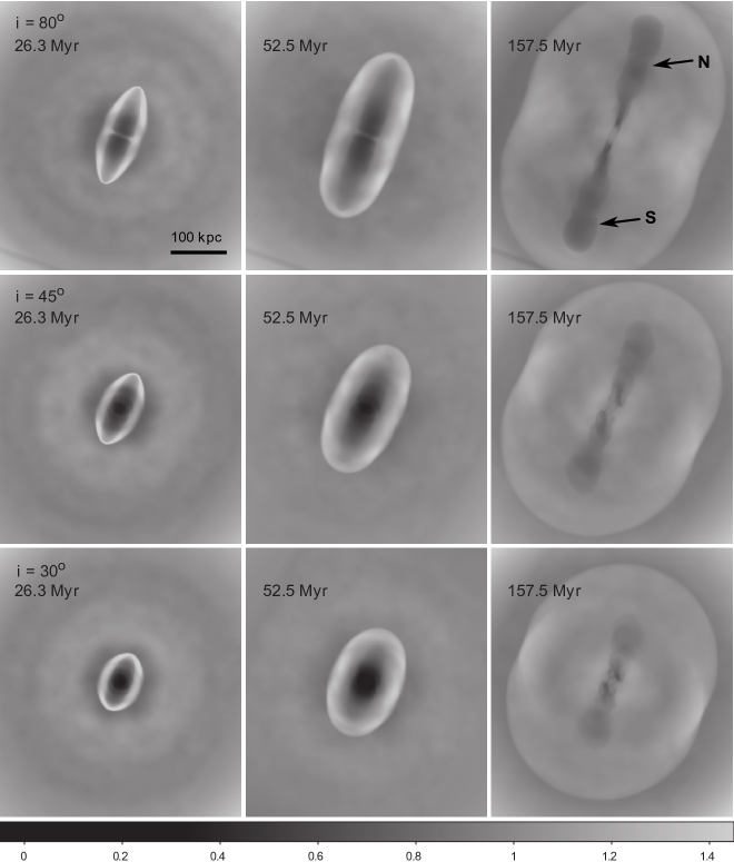
Figure 1: Synthetic observations of the RE simulation at three epochs and three orientations from the energy band 1.5-2.5 keV. Each row corresponds to one inclination angle with the time progressing from left to right. The observations were divided by a best-fit double $\beta-$profile to emphasize the X-ray cavities. The N and S cavity labels distinguish the cavities from each jet.

Synthetic X-ray observations of the RE, relic simulation are shown for several times and projection orientations in Figure 1. Following a common practice designed to highlight AGN-blown cavities, the computed brightness distribution of the ICM outside of the identified cavities was fit with a double $\beta$-profile (§4.1) and then divided out to accentuate the X-ray cavities. The double $\beta$-profile was determined independently for each synthetic X-ray observation. Figure 1 shows the synthetic X-ray observations in a 1.5-2.5 keV band divided by the best-fit double $\beta-$profile in each instance. Time evolution of the system is displayed from left to right. At the earliest time shown, 26.3 Myr, the jets had just turned off. Each row corresponds to a different orientation, with the inclination angle of the jet with respect to the line of sight decreasing from top to bottom. There are several notable features in each observation. Cavities are seen as brightness decrements from the surrounding emission. A pair of cavities is seen at 26.3 and 52.5 Myr at large inclination but appear to merge into a single cavity at small inclination. Presumably X-ray emission from a central galaxy would prevent the two cavities from appearing as a single cavity. Our simulations, however, do not include emission from gas bound specifically to the central galaxy. All inclinations show a pair of cavities at 157.5 Myr. The contrast in brightness of the cavity to the surrounding gas diminishes with both distance from cluster center and decreasing inclination. A detailed discussion on these trends can be found in Enßlin & Heinz (2002). The bow shock from the jets is seen in all observations. At early times the bow shock appears as a bright rim surrounding the cavities. At later times the bow shock has moved far from the edge of the cavities and no longer appears as a bright rim.

3.2 Intermittent (I13) Observations

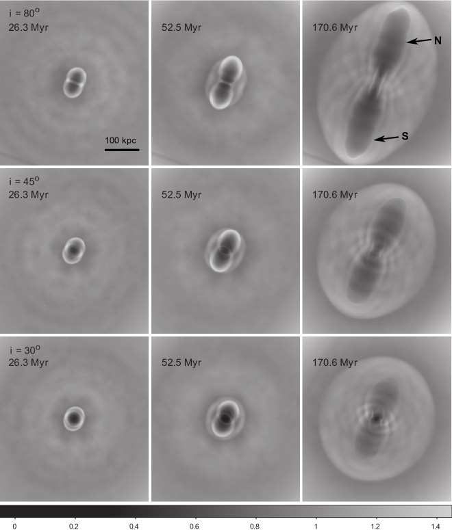
Figure 2: Synthetic observations as in Figure 1 of the I13 simulation.

Figure 2 shows a similar set of observations to those in Figure 1, but for the I13, intermittent jet simulation. Several new features are seen with the introduction of jet intermittency. Late times at every inclination reveal “ripples” between the cavities and the bow shock. These features correspond to sound waves generated at the cavity walls during periods of jet activity. Similar “ripples” have been seen in observations of the Perseus cluster (Fabian et al. (2003)). A second, related distinction from the RE observations is the appearance of bright rims outlining the cavities at every epoch. At smaller inclination angles the bright rims resemble the “arms” seen on smaller scales in NGC 4636 (Baldi et al., 2009).

4 Cavity Measurements

In the following analysis we attempted to apply common techniques for extracting two fundamental parameters for each cavity detected in each observation throughout the elapsed time of each jet model. Every epoch for a given simulation represents a separate test for measuring both cavity enthalpy and cavity age. Following this time evolution allows us to detect biases and trends in the quality of the measurements. For the remainder of this paper we refer to values measured directly from the simulation data as the “actual” values, while values measured from the synthetic observations are referred to as “observed” values. We report the fractional error on a measured quantity $x$ as $\epsilon_{x}\equiv(x_{observed}-x_{actual})/x_{actual}$ for the remainder of this paper.

4.1 Enthalpy

The minimum energy required to produce a cavity is generally estimated as the total thermal energy in the cavity and the work done inflating the cavity slowly at constant pressure; that is, the enthalpy in the cavity, $H=U_{therm}+PV\sim{\rm several}\times PV$. In particular, if the adiabatic index of the cavity plasma is $\gamma_{c}$,

$$H=\frac{\gamma_{c}}{\gamma_{c}-1}PV.$$ (8)

For a gas with $\gamma_{c}=5/3$, applicable to our simulations, this gives $H=(5/2)PV$. Estimation of cavity enthalpy, under the assumption that the cavity was inflated at its current location, requires knowledge of both the cavity volume and surrounding gas pressure. Since the AGN activity disturbed large volumes of the ICM it is not straightforward to determine either its pressure distribution or, for that matter, the volume occupied by the AGN generated cavity. A common strategy to resolve these two problems involves fitting a simple, symmetric brightness profile to regions of emission that seem not to include cavity structures. That profile can then be used to obtain estimates for the average radial ICM properties. There are several variations of this strategy (e.g., Wise et al., 2004; Bîrzan et al., 2004). Our goal was not to determine the best strategy but to use a common approach as an example. We followed a procedure similar to Wise et al. (2004) and Xue & Wu (2000) to extract pressure and Bîrzan et al. (2004) to extract volume from each observation.

For this exercise we used a double $\beta-$profile profile (e.g., Ikebe et al., 1996) of the form

$$S_{X}(r_{p})=S_{0}\left(S_{01}\left[1+\left(\frac{r_{p}}{R_{C1}}\right)^{2}\right]^{1/2-3\beta_{1}}+S_{02}\left[1+\left(\frac{r_{p}}{R_{C2}}\right)^{2}\right]^{1/2-3\beta_{2}}\right),$$ (9)

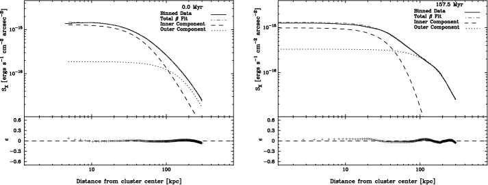
Figure 3: Double $\beta-$profile fits to azimuthally averaged radial brightness brightness distributions measured from the synthetic X-ray observations. On the left is the fit for the initialized cluster of both RE and I13 observed at an inclination of 80${}^{\text{o}}$. On the right is a fit for the RE simulation at 157 Myr observed at an inclination of 45${}^{\text{o}}$. The bottom panel of each plot shows the fractional error of the fit to the observed distribution.

where $r_{p}$ is the projected distance from cluster center, to model the brightness distribution of the X-ray emitting ICM. Xue & Wu (2000) discuss the benefits of using this profile as opposed to a single $\beta-$profile. The profile was fit independently to each 1.5-2.5 keV synthetic X-ray observation of the RE and I13 simulations. The synthetic images were divided into annular bins, each $\approx$ 1 arc sec in width. To remove any effects of the X-ray cavities in characterizing the brightness profile of the cluster plasma, a set of ellipses was chosen that best fit each cavity by eye. Any pixels within these ellipses were excluded from the annular bins. The average flux from the remaining pixels was used to define an azimuthally averaged brightness profile that was fit with the double $\beta$-profile. Refer to Appendix A for details regarding the fitting procedure. Figure 3 shows example double $\beta-$profile fits for observations of both models at an inclination of $i$ = 45${}^{\text{o}}$. The best fit profiles resulted in $0.5\leq\beta_{1}\leq 1.5$, $0.9\leq\beta_{2}\leq 1.8$ with typical values $R_{C1}\sim 50$ kpc, $R_{C2}\sim 200$ kpc, $S_{01}\sim 0.8$, and $S_{02}\sim 0.2$. The undisturbed cluster parameters were $\beta_{1}=0.7$, $\beta_{2}=1$, $R_{C1}=55$ kpc, $R_{C2}=260$ kpc, $S_{01}=0.9$, and $S_{02}=0.1$.

4.1.1 Cluster Temperature Profile

The ICM temperature, $T_{ICM}$, at a given projected radius, $r_{p}$, was determined from the ratio of fluxes in two bands; 1.5-2.5 keV and 9.5-10.5 keV. In particular, the equation

$$\frac{S_{X,1.5-2.5}(r_{p})}{S_{X,9.5-10.5}(r_{p})}=\frac{\int_{\nu=(1+z)1.5\,keV/h}^{\nu=(1+z)2.5\,keV/h}g_{ff}(\nu,T_{ICM})e^{-h\nu/T_{ICM}}d\nu}{\int_{\nu=(1+z)9.5\,keV/h}^{\nu=(1+z)10.5\,keV/h}g_{ff}(\nu,T_{ICM})e^{-h\nu/T_{ICM}}d\nu}$$ (10)

was solved for $T_{ICM}$ using the aforementioned double $\beta$-profile fits. Following Wise et al. (2004), we assumed that the two components of the double $\beta$-profile corresponded to two phases of the ICM with temperatures $T_{ICM,1}$ for the inner component and $T_{ICM,2}$ for the outer component. $T_{ICM,1}$ was taken to be the minimum and $T_{ICM,2}$ the maximum temperatures found using Equation 10. The projected radius for the transition from $T_{ICM,1}$ to $T_{ICM,2}$ was chosen to be the average of $R_{C1}$ and $R_{C2}$. Figure 4 shows a comparison between the actual azimuthally averaged temperature profile as a function of physical radius from the RE initial conditions and the two component projected profile. Note that $T_{ICM,1}$ mostly exceeded the actual inner core temperatures, since hotter gas along the line of sight contaminated $S_{X}$ at small $r_{p}$.

4.1.2 Cluster Electron Density Profile

The radial thermal electron density profile of component $i=1,2$ was obtained by inverting equation (9), following the derivation of Xue & Wu (2000);

$$n_{ei}^{2}(r_{p}=0)=\left(\frac{4\pi^{1/2}}{\alpha(T_{ICM,i})g_{i}\mu_{e}}\right)\left(\frac{\Gamma(3\beta_{i})}{\Gamma(3\beta_{i}-1/2)}\right)\left(\frac{S_{0i}}{R_{Ci}}\right)A_{ij},$$ (11)

where

$$\alpha(T_{ICM,i})=\frac{2^{4}e^{6}}{3m_{e}\hbar c^{2}}\left(\frac{2\pi\,1.602\times 10^{-9}\,T_{ICM,i}}{3m_{e}c^{2}}\right)^{1/2},$$ (12)

$$g_{i}=\int_{\nu=(1+z)1.5\,keV/h}^{\nu=(1+z)2.5\,keV/h}g_{ff}(\nu,T_{ICM,i})\,e^{-h\nu/T_{ICM}}\,d\nu,$$ (13)

and

$$\frac{1}{A_{ij}}=1+\frac{R_{Ci}S_{0j}g_{i}}{R_{Cj}S_{0i}g_{j}}\left(\frac{T_{ICM,i}}{T_{ICM,j}}\right)^{1/2}\left[\frac{\Gamma(3\beta_{j})\Gamma(3\beta_{i}-1/2)}{\Gamma(3\beta_{i})\Gamma(3\beta_{j}-1/2)}\right],$$

$$j=1,2\,\,and\,\,j\neq i.$$ (14)

The values for $S_{0i}$, $R_{Ci}$, and $\beta_{i}$ were the best fit values for each component from the 1.5-2.5 keV observation. For simplicity, we assumed pure hydrogen. The electron weight, $\mu_{e}=2/(1+X)$, where $X$, the hydrogen mass fraction, was therefore unity. The total electron density at a projected radius $r_{p}$ was determined by

$$n_{e}(r_{p})=\displaystyle\sum_{i=1}^{2}n_{ei}(r_{p})=\left(n_{e}(r_{p}=0)\displaystyle\sum_{i=1}^{2}n_{ei}(r_{p}=0)\left[1+\left(\frac{r_{p}}{R_{Ci}}\right)^{2}\right]^{-3\beta_{i}}\right)^{1/2}.$$ (15)

Figures 5 and 6 show example observed electron density profiles determined by Equation 15 compared to the actual azimuthally averaged electron density from the RE simulation from observations at $i$ = 45^°. The data for the actual density were generated considering only computational zones with $C_{jet}$ = 0 (pure ICM plasma) to avoid any contamination by AGN plasma. Near to and within the jet launching region, $\lesssim\,l_{jet}$, this condition was, of course, not met while the jets were active. For this reason there are no data points at small radii in Figures 5 and 6 when the jets were active.

The initial conditions in the upper left panel of Figure 5 reveal a bias towards lower density within the inner core radius (${\lesssim}$ 50 kpc) with a fractional error $\epsilon_{\rho}\sim$ 15%. This is a result of the bias toward higher temperatures in the determination of $T_{ICM,1}$ discussed in §4.1.1. By holding $j_{\nu}$ constant in Equation 7 for an observation with $h\nu_{local}$ approximately equal to the actual gas temperature it can be shown that an overestimate of the gas temperature will result in an underestimate of the electron density. After jet activity terminated in the RE simulation, the observed density profile matches the actual ICM profile with an error, $\epsilon_{\rho}\sim$ 30%. The largest contribution to the error is from regions influenced by the bow shock. Excluding these regions gives $\epsilon_{\rho}\lesssim$ 15%. Evidence of the bow shock is seen in the actual density profile as a bump in excess of the smooth, observationally determined profile at $r_{p}$ = 35 kpc for 26.3 Myr, 70 kpc for 52.5 Myr, and 200 kpc at 157.5 Myr. These distances correspond to the cluster-centric distance of the bow shock orthogonal to the jet axis. In general, the observed distribution closely matches the actual distribution for radii outside the inner core radius, $R_{C1}$, at all times also with $\epsilon_{\rho}\lesssim$ 10%.

The I13 profiles in Figure 6, similarly display fractional errors for the observed distribution $\epsilon_{\rho}\lesssim$ 15% at all times exterior to $R_{C1}$. Evidence of the bow shock is seen here as well in the actual profile as a bump in excess over the observed profile at $b$ = 20 kpc for 26.3 Myr, 55 kpc for 52.5 Myr, 100 kpc for 105 Myr, and 200 kpc for 170.6 Myr. The electron density profile of the ICM obtained from the brightness profile was reliable to within $\sim$ 20% outside of regions influenced by shocks regardless of jet intermittency and observed inclination. Inside of shock influenced regions the fractional error was as high as $\sim$ 40%.

4.1.3 Cluster Pressure Profile

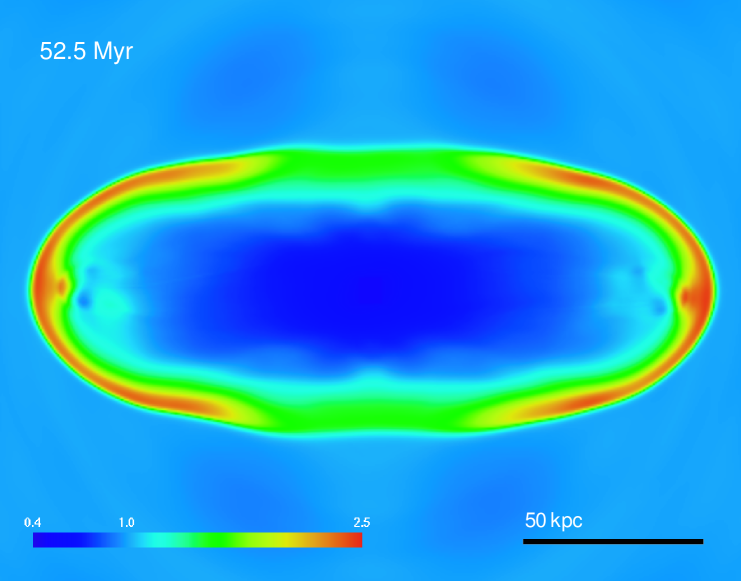
Figure 9: A slice through the midplane of the computational box showing the ratio of the pressure at 52.5 Myr into the RE simulation to the initial conditions. The pressure within 50 kpc of the cluster center has dropped by $\sim$20% from the initial conditions. The bow shock is visible as an increase in pressure by a factor of $\sim$ 2.5 from the initial conditions. (A color version of this figure is available in the online journal.)

The (azimuthally averaged) radial ICM pressure profile was calculated for each observation from the double $\beta$-profile model temperature and density profiles just outlined, assuming an ideal gas equation of state. Figures 7 and 8 show example pressure profiles determined from the observed temperature and density profiles along with azimuthally averaged ICM pressures and AGN pressures extracted directly from the RE and I13 simulation. Following the procedure used for density, only zones with $C_{jet}$ = 0 (pure ICM plasma) were used to measure the ICM pressure profile. Zones with $C_{jet}\geq$ 0.01 were used to measure the AGN pressure profile. The top left panel of Figure 7 shows the results of the double $\beta$-profile inversion (the “observed” profile) for the initial conditions. Within $R_{C1}$ the observed profile underestimates the actual ICM profile by $\gtrsim$ 10%. This is due to the underestimate of the electron density discussed in §4.1.2. Outside of $R_{C1}$ the ICM pressure profile is measured with $\epsilon_{P}\leq$ 10%. At the time the jets are turned off for the RE simulation, the top right panel of Figure 7, the ICM pressure is measured with $\epsilon_{P}$ $<$ 20% at all radii. The signature of the bow shock in the ICM (solid line) can be seen at 35 kpc as a bump in excess over the observed profile. At 52.5 Myr, the lower left panel, the observed profile significantly overestimates the ICM pressure by $\epsilon_{P}$ $>$ 10% within $R_{C1}$. The pressure $\sim$ 35 kpc behind the bow shock has dropped $\sim$ 20% from the initial conditions at this time as seen in Figure 9. By 157.5 Myr, the ICM has relaxed closer to equilibrium, and the observed profile measures the actual pressure to $\epsilon_{P}\leq$ 15%.

The observed pressure profiles for the I13 simulation shown in Figure 8 reproduced the ICM profile to $\epsilon_{P}\leq$ 45% at all times, and at distances $\gtrsim 20-30$ kpc from cluster center the observed profile was typically much better than that. The intermittency of the jets in the I13 run produced a more complex pressure distribution than the RE simulation. It cannot be captured by the smooth profile produced by the double $\beta-$profile inversion. At 52.5 and 105 Myr, the actual pressure varies $\pm$30% from the observed pressure within $R_{C2}$. By 170.6 Myr, the strength of the bow shock has diminished, and the error on the observed profile falls to $\epsilon_{P}\leq$ 10% outside $R_{C1}$. Inside of $R_{C1}$, however, the effects of the AGN activity produces a pressure structure poorly reproduced by the observed profile. The measurement of the ICM pressure profile from observation was reliable to within $\sim$ 20% outside of regions strongly affected by jet related shocks. Inside of shocked regions the measurement was only reliable to within $\sim$ 60%. This was true for both the RE and I13 simulations regardless of the observation orientation.

Following convention, the observed ICM pressure profiles were used to calculate X-ray cavity enthalpy on the assumption that the ICM and cavity pressures were equal. The dotted lines in Figures 7 and 8 show the average pressure in AGN plasma at each radial bin. This pressure could only be observationally measured if the cavity were in exact pressure balance with the ICM and the exact cluster-centric distance of the cavity was known. Here we discuss how closely observation matches the AGN plasma profile assuming the cavity location is known. §4.1.5 discusses the effect of projection on inferred pressure.

The AGN plasma pressure in the RE simulation, as shown in Figure 7, roughly follows the ICM pressure at 26.3 and 157.5 Myr except for high pressure at the ends of the jets where momentum flows drive the cavities outward (OJ10). At 52.5 Myr, the AGN plasma pressure differs by as much as a factor of three from the actual ICM pressure from 30-100 kpc. This discrepancy can be explained by the influence of the bow shock. Referring to Figure 9, shocked ICM material between projected distances of 30-100 kpc raised the average ICM pressure over the lower pressure inside of the jet cocoon. The observed pressure profile, which is sensitive to the ICM pressure, is $\sim$ 75% greater than the AGN plasma pressure within $R_{C1}$ at this time.

For the I13 simulation at 26.3 Myr in Figure 8, there is a significant difference between the AGN and ICM profiles from 25-35 kpc also due to the effects of the bow shock. At this time the observed pressure profile overestimates the AGN plasma pressure by $\sim$ 50% within 20 kpc. At 52.5 Myr, the AGN and ICM profiles approximately agree with the exception at the ends of the jets. Here the observed profile matches the actual AGN plasma pressure to within 13%. The observed, AGN, and ICM profiles all agree at 52.5 Myr to within $\sim$ 30% except the ends of the jets. The intermittency of the jets impacts how well the observed profile reproduces the AGN pressure. At 105 Myr, when the jets are inactive, the observed pressure overestimates the AGN pressure within 30 kpc while at 170.6 Myr, when the jets are active, it underestimates it. Inferring AGN plasma pressure from observational measurement of the ICM pressure at a specific radius was reliable only to $\sim$ 75% from the RE and I13 observations.

4.1.4 Cavity System Volume

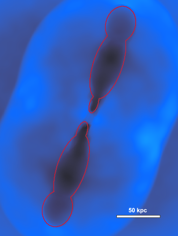
Figure 10: Example of area enclosed by ellipses fit by eye (solid line) to a 1.5-2.5 keV observation of the RE simulation at 131.3 Myr divided by a best-fit double $\beta-$profile. (A color version of this figure is available in the online journal.)

Cavity volumes were estimated from 1.5-2.5 keV observations at each analyzed epoch for both RE and I13 simulations. As already noted, each cavity was fit by eye with a set of ellipses (Bîrzan et al., 2004). For each projection angle, $i=80^{\arcdeg},45^{\arcdeg},~{}{\rm and}~{}30^{\arcdeg}$, the cavities were assumed in this measurement to be in the plane of the sky in order to test the effects of an inaccurate or unknown value for the inclination. These observed cavity volumes were calculated assuming them to be ellipsoids of revolution around the major axis of each projected ellipse. By using multiple ellipses to cover each projected cavity we were better able to define the outer edge of the X-ray cavity. Figure 10 shows an example of the area enclosed by the ellipses chosen for the RE simulation at 131.3 Myr observed at $i$ = 80${}^{\text{o}}$. In general, it was difficult to define the edge of the cavities for the RE simulation once the cavities extended past $R_{C1}$. For the I13 simulation the cavities were often outlined with a bright rim (see Figure 2), making the edge (taken to be the inside of the rim) easier to find.

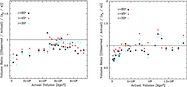
Figure 11: The observationally determined total cavity volume to the actual total cavity volumes from each every analyzed epoch for the RE simulation (left) and the I13 simulation (right). (A color version of this figure is available in the online journal.)

The actual cavity volumes were computed by integrating the volume in the simulation data with $C_{jet}\geq 0.01$ (partially AGN plasma). Observed and actual volumes are compared in Figure 11. Since we expect a projection bias due to foreshortening along the jet axis (see Appendix B), we plot the observed volume divided by $a_{p}/a$, where $a_{p}$ is given by Equation B6 and $a$ is the actual length of a single best fit ellipse, normalized by the actual volume. The scatter in the measurements without correcting for this projection bias was $\sim$ 50%. Two features stand out in the comparisons in Figure 11. First, the $a_{p}/a$ correction reduced the scatter due to the projection bias to approximately 10-15% for both RE and I13. The second obvious feature of the comparison is that the observed cavity volume estimates tend to be modestly smaller than the actual volumes for RE but not for I13. The reason for this has to due with the different shapes of the cavities between RE and I13. I13 retains a nearly elliptical area at all times while RE developed a non-elliptical shape (see Figures 1 and 2), which required many ellipses to fit. Fitting ellipses will tend to underestimate a non-elliptical shape if the observer requires that none of the fits extend beyond the cavity edge. Despite this limitation, and the subjective, observer-dependent nature of the process, our observed volume estimates generally agree with the actual volumes to within about $\pm 50$% (omitting the $a_{p}/a$ correction).

The observations used to determine cavity analysis did not include any noise representing X-ray counts or intrumental effects. Low counts at large cluster centered distances would make cavity edges in those regions more difficult to identify. The long axis of all of the observed cavities, roughly aligned with the jet, would likely be underestimated given these conditions, which would reduce the measured volume by the same amount.

4.1.5 Cavity System Enthalpy

The observational estimates for the ICM pressure profile and cavity system volume presented above were used to derive the total cavity enthalpy, $H_{obs}$. The cavity volume enclosed by the chosen ellipses for each observation was discretized into 1 kpc³ volume elements corresponding to the 1 arc sec resolution of the images for a cluster distance, $D_{L}$ = 240 Mpc. The pressure in each cavity volume was determined from the observed pressure profile and the projected cluster-centric distance of the volume elements. The total enthalpy in the cavity system for each observation was given by

$$H_{obs}=\frac{5}{2}\displaystyle\sum_{i}^{N_{elements}}P_{i}\left(1\,kpc^{3}\right).$$ (16)

Figure 12 shows comparisons of the total energy added to the simulation volumes by jets, $\Delta E_{tot}$, the actual enthalpy in the cavity systems, $H_{act}$, and the above observed cavity enthalpy estimates, $H_{obs}$, throughout the RE and I13 simulations at three inclinations. The value for $H_{act}$ was computed from the pressure and total volume of each voxel in the simulation data with $C_{jet}\geq 0.01$ to be consistent with the synthetic observations (see §3). This conservative cut meant that some ICM enthalpy was included in $H_{act}$ values, making it possible for $H_{act}>\Delta E_{tot}$.

Several features stand out in comparing the various energy measures. The first feature is that $H_{obs}$, $H_{act}$, and $\Delta E_{tot}$ all agree with each other within about a factor of two for a given simulation and inclination angle. Second, the comparisons of enthalpy, both observed and actual, and the total energy measures is better for the intermittent jet simulation, I13, than for the terminated, RE, case. This is consistent with the analysis of the simulations reported in OJ10. In particular, they noted that about 50% of the jet energy ($\Delta E_{tot}$) injected during the active phase of either the I13 or RE model had been converted into ICM thermal or kinetic energy by the end of the simulation. The remaining energy increment was mostly gravitational potential energy in the ICM or thermal energy in the jet cocoon, which is roughly what $H_{obs}$ measures. Approximately 30% of $\Delta E_{tot}$ ended up as gravitational potential energy in the ICM for the RE simulation. By contrast, a much smaller fraction, $\sim 15$%, of $\Delta E_{tot}$ in the intermittent jet, I13, simulation is converted to ICM gravitational by the simulation’s end. Thus, we should expect a closer match between $\Delta E_{tot}$ and $H_{act}$ in that case.

Another striking feature for both panels of Figure 12 is the consistency in $H_{obs}$ among the inclination angles for a given simulation and epoch. This is due to two competing projections effects. In particular, the estimated volume generally decreases with decreasing inclination angle as discussed in §4.1.4, while the projected distance from cluster center decreases, making a cavity appear to be in a higher pressure environment then it actually is. To see the net effect refer to Figures 7 and 8. It is evident that the ICM pressure profile can be approximated as a power law, $P=P_{0}(r/r_{0})^{\alpha}$, over the projected distances the cavities occupy (40-200 kpc) for most of the simulated time. Then, assuming a given cavity is a cylinder with radius $R$ extending from a projected distance $r_{1}\,sin\,i$ to $r_{2}\,sin\,i$ (see Appendix B regarding the use of $sin\,i$) and estimating $\alpha\approx$ -1 we would predict that the enthalpy $H$ would be

$$H =\pi\frac{5}{2}\,R^{2}\,p_{0}\int_{r_{1}\,sin\,i}^{r_{2}\,sin\,i}\left(\frac{r}{r_{0}}\right)^{-1}\,dr$$ (17)

$$=\pi\frac{5}{2}\,R^{2}\,p_{0}ln\left(\frac{r_{2}}{r_{1}}\right),$$ (18)

which is independent of $i$.

For the RE simulation on the left panel of Figure 12 $H_{obs}$ always underestimated $H_{act}$ while the jets were active. Recall that $H_{obs}$ depends on the observed estimate of the ICM pressure distribution and, from §4.1.3, that the observed pressure profile underestimated the AGN plasma pressure (the cavity pressure) while the jets were active. In short, during those times the cavities are over-pressured as they drive moderate strength shocks into the ICM. This is consistent with comparisons shown in Figure 7. Further into the simulation we see $H_{act}$ declining. The cavities are rising buoyantly in the cluster while maintaining approximate pressure equilibrium (see OJ10). The thermal energy in the cavities dropped as this energy was transferred to gravitational potential energy. The observed values follow this trend, remaining within $\approx$ 50% $H_{act}$.

The I13 simulation on the right panel of Figure 12 shows a different evolution of $H_{act}$ and $H_{obs}$ because of the different AGN history. There is a step-like growth of $H_{act}$ due to the intermittency of the jets. The time delay between the peaks of $H_{act}$ and $H_{obs}$ at each step is due to the difference in evolution of the observed ICM pressure and the actual AGN plasma profiles. When the jets turn on the cavities are over-pressured with respect to the ICM, but they eventually expand to approximate pressure balance. Prior to the expansion of the cavities, however, the higher energy content of the cavities cannot be accurately measured by the procedure described in §4.1.3. Therefore, an increase of $H_{obs}$ lags behind an increase of $H_{act}$.

4.2 Ages

Three characteristic timescales are commonly employed for determining cavity age. For a cavity centered at a projected distance $r_{p}$ from cluster center, radius $R$, cross section $S$, drag coefficient $C$, and volume $V$ these times are: 1) the buoyant rise time $t_{buoy}\approx r_{p}\sqrt{CS/(2gV)}$, 2) the “refill time” $t_{r}=2\sqrt{R/g}$, and 3) the sound crossing time $t_{c}=r_{p}/c_{s}$ (Bîrzan et al., 2004). These times can be compared to known ages from the simulations given measurements of the sound speed, $c_{s}$, and $g$ from the synthetic observations. Measurements of each age were made from observations of the N and S cavities (see Figures 1 and 2) at the end of the RE simulation, $t=157.5$ Myr, and I13 simulation, $t=170.6$ Myr, at three different inclination angles. In these observations we represented each cavity as a single ellipsoid with semi-major axis $a$ and semi-minor axis $b$. Following a procedure similar to Bîrzan et al. (2004), the value of $r_{p}$ was the projected distance from cluster center to the center of the cavity, the radius was given by $R=\sqrt{ab}$, and the cross section was given by $S=\pi\,b_{max}^{2}$, where $b_{max}$ was half the maximum azimuthal width of the cavity. The volume $V$ was determined for each cavity following the method described in §4.1.4. The sound speed was given by $c_{s}=\sqrt{\gamma k<T_{ICM}>/(\mu m_{H})}$. At the end of the RE simulation $<T_{ICM}>=$ 2.77 keV giving $c_{s}$ = 941 km s^-1, and at the end of the I13 simulation $<T_{ICM}>=$ 2.82 keV, giving $c_{s}$ = 950 km s^-1. Refer to Appendix C for details on estimating $g$, which we assumed to be constant, from the synthetic observations. We let $C$ = 1 for simplicity.

Table 1 shows the measured parameters and age estimates for each observation at the end of the RE and I13 simulations. Both $t_{buoy}$ and $t_{c}$ are affected by projection. For this reason, we would expect the buoyant rise time to vary as $t_{buoy}\propto r_{p}/\sqrt{a}\propto\sqrt{sin\,i}$ due to projection effects on both the projected distance and semi-major axis of the cavity. The sound crossing time, however, should vary more rapidly with inclination as $t_{c}\propto r_{p}\propto sin\,i$. The cavity pairs for both simulations approximately show this trend for $t_{buoy}$ and $t_{c}$. The refill time shows a weaker dependence on inclination angle because $t_{r}\propto\sqrt{(ab)^{1/2}}\propto(sin\,i)^{1/4}$ (recall that we assumed constant $g$ in calculating ages). An important aspect of Table 1 was that for most cases $t_{buoy}<t_{c}$, which implies a terminal buoyant velocity greater than the sound speed. This unphysical result could have been avoided in a number of ways. In their analysis of Hydra A, for example, Wise et al. (2007) represented the cavity system as a series of spherical bubbles. Approximating the end of the N cavity of the RE simulation observed at $i$ = 80${}^{\text{o}}$ as a sphere would increase $r_{p}$ to $\sim$ 200 kpc and would decrease $V$ to $(4/3)\pi\,r^{3}\sim 1.4\times 10^{5}$ kpc³. Given these measurements for an outer spherical cavity, $t_{buoy}\sim$ 244 Myr while $t_{c}\sim$ 208 Myr. Another approach may have been to assume $C>$ 1 similar to values empirically estimated by Jones & DeYoung (2005). The parameters and measurements used in a buoyant rise model are not very well constrained. A buoyant model also did not properly capture the evolution of the cavities in the RE or I13 simulations (see OJ10). For these reasons we chose not to use $t_{buoy}$ as the cavity age. The equations for $t_{r}$ and $t_{c}$ are related, and the models only differ in the length over which material moves. By convention, $t_{r}$ uses the cavity radius, which is not affected by projection. We instead use the values of $t_{c}$ for the cavity ages in subsequent calculations so that our analysis demonstrates the dependence on projection. When projection did not greatly effect our measurements $t_{c}$ was reliable to within $\pm 20$%.

4.3 Cavity Power

The enthalpy and age of a cavity system are typically combined into a characteristic power called the cavity power $P_{cav}=H/t$. If $P_{cav}$ can be deposited into the ICM it may balance the cooling in the host cluster. It is therefore common practice to compare $P_{cav}$ with the cooling (e.g., Bîrzan et al., 2004; Rafferty et al., 2006; Cavagnolo et al., 2010). The cavity power should represent a lower limit to the total luminosity of the AGN because it does not account for energy already deposited into the ICM or other forms of AGN plasma energy such as magnetic, potential, or kinetic (see §4.1.5). Table 2 shows a comparison of the observed $P_{cav,obs}$ with the actual total average jet luminosity, $L_{jet,act}$, for both RE and I13 observed at the three different inclinations at the end of each simulation. $P_{cav,obs}$ was computed as $H_{obs}/\langle t\rangle$, where $\langle t\rangle$ was the average of the ages in Table 1 for the N and S cavities, while the mean jet power, $L_{jet,act}=\Delta E(t)/t$, where $t$ = 157.5 Myr and $t$ = 170.6 Myr for the RE and I13 simulations respectively. The differences between $P_{cav,obs}$ and $L_{jet,sim}$ at these times were characteristic of early times.

Observations of the RE and I13 simulations produced $P_{cav,obs}$ increasing with decreasing inclination primarily due to projection effects on measuring the ages as discussed in §4.2. For the RE simulation, $P_{cav,obs}<L_{jet,act}$ as we would expect for all but the smallest inclination angles. The I13 observations, however, resulted in $P_{cav,obs}>L_{jet,act}$ at all orientations. The underestimate of cavity system age was the dominant reason $P_{cav,obs}$ exceeded $L_{jet,act}$ in these observations. For measurements from observations at $i$ = 80${}^{\text{o}}$, when the error on the assumed inclination is small, $P_{cav,obs}$ was within $\sim$ 40% of $L_{jet,act}$, and $P_{cav,obs}$ was within a factor of three of $L_{jet,act}$ across all of the observed inclination angles.

5 Conclusions

We have presented an analysis of the reliability of common techniques used to extract X-ray cavity enthalpy, age, and mechanical luminosity from X-ray observations of cavity systems. By utilizing synthetic X-ray observations of detailed simulations we were able to directly compare observationally determined and actual values from the simulations. The important results from this work are:

$\bullet$ The synthetic observations of the I13 simulation show bright rims outlining the cavities at each analyzed epoch out to 170.6 Myr while the RE simulation does not show bright rims. The difference in the AGN history represented by each model accounts for this difference. I13 had periodic injection of energy into the cavities throughout the simulation while RE deposited all of its energy early on.

$\bullet$ Observationally measuring X-ray cavity enthalpy is reliable to within approximately a factor of two across a wide range of age and inclinations for the models of jet intermittency presented here. Several steps go into determining the enthalpy, and each may introduce significant errors. Extracting the ICM electron density profile, for example, was reliable to within $\sim$ 20% outside of regions strongly influenced by shocks. Inside recently shock influenced regions the error was $\sim$ 40%. Combining this and the temperature profile into the pressure inside of the cavity at a given cluster-centric distance may not be as accurate. During periods of jet activity, the observationally determined pressure may differ by as much as $\sim$ 75% from the cavity pressure. This is related to the supersonic speeds of the jets through the ICM and the consequent post-shock pressure enhancement. Our measurements of cavity volume were within $\pm$50% of the actual total cavity system volume. This process is subjective, however, and a more robust and objective method for finding and outlining cavities should be developed. The overall effect of each of these measurements is contained in the factor of two reliability of enthalpy measurements. The energy required to offset cooling in clusters can be characterized as $\eta PV$. An approximate factor of two span in $\eta$ in our tests is due largely to uncertainties in the measurement of $PV$.

$\bullet$ The determination of cavity age from one or more of the commonly used age estimates could potentially be misleading. The buoyant rise model was not an accurate description of the evolution of the cavities in our simulations. A simple application of this model implied unrealistic terminal velocities greater than the sound speed. The refill time model produced ages within $\pm$15% of the correct age regardless of the error on assumed inclination. It relied on an accurate measurement of the gravitational acceleration, however, which assumes the cluster to be in hydrostatic equilibrium. This assumption may be not be valid for a given cluster. We preferred to use the sound crossing time as a simple and fairly robust model for cavity age. For a well constrained inclination angle, our measurements were within $\pm$20% of the actual cavity age.

$\bullet$ Observationally measuring the cavity power produced values within a factor of $\sim$ 3 of the average total jet luminosity from our simulations regardless of assumed inclination angle. The observed cavity power was within 40% of the jet luminosity if the projection effects were negligible. At all observed inclination angles for the I13 simulation and $i$ = 30${}^{\text{o}}$ for the RE simulation the cavity power overestimates the average jet luminosity largely due to underestimates in the cavity system age.

Appendix A Fitting $\beta$ Profiles

To calculate a best fit to the brightness distributions comparable with observations, the flux from the synthetic observation was scaled by the net counts from Chandra observations of Hydra. Counts were taken from the $evt2$ files in the Chandra archive (ObsIDs 575 and 576, Chandra calibration program; ObsIDs 4969 and 4970, program 05800556, P.I. McNamara) (Wise et al., 2007). The total number of counts with energies from 1.5-2.5 keV in a circular region centered on the cluster with a diameter equal to the size of the synthetic observations, 12.3 arc min a side, was extracted for each observation. A total of $N_{c}=451345$ counts for the four observations were detected in this region over 227 ksec. The scaling factor $\xi$ was calculated as

$$\xi=\frac{N_{c}\,\,counts}{\displaystyle\sum_{i}^{N_{pixels}}S_{i}\,\,erg\,s^{-1}\,cm^{-2}},$$ (A1)

where $S_{i}$ is the flux for a given pixel observed over a band from 1.5 to 2.5 keV. $\chi_{norm}^{2}$ was then calculated from the simulated average counts in a bin, the product of $\xi\langle S_{i}\rangle$, assuming Poisson statistics. The downhill simplex method was used to minimize $\chi_{norm}^{2}$ by simultaneously fitting $S_{0i}$, $R_{C,i}$, and $\beta_{i}$. Both the RE and I13 grids extended only 300 kpc. To ensure that our fits were not affected by the truncation of the atmosphere, additional azimuthally averaged data points were generated from a synthetic observation of the cluster discussed in §2.2 extending the initial conditions to 600 kpc.

Appendix B Projected Semi-major Axis of an Ellipsoid

The projected semi-major axis of revolution of an ellipsoid can be determined from the inclination angle, $i$, and the un-projected aspect ratio taken to be $\psi=a/b$, where $a$ is the semi-major axis and $b$ is the semi-minor axis along the other two dimensions. Figure 13 shows an example of the geometry of the problem where the line segment $OC$ is the projected semi-major axis. We start with an ellipse defined by

$$\frac{x^{2}}{a^{2}}+\frac{y^{2}}{b^{2}}=1$$ (B1)

lying in a plane that includes the line of sight with a tangent line of slope

$$\frac{dy}{dx}=-\frac{a^{2}}{b^{2}}\frac{y}{x}=-\psi^{2}\frac{y}{x}=tan\,i$$ (B2)

from the observer. The coordinates $D=\{x_{0},y_{0}\}$, where the tangent line intersects the ellipse, are given by

$$x_{0}=-\left(\frac{1}{\psi^{4}tan^{2}i\,b^{2}}+\frac{1}{a^{2}}\right)^{-1/2},y_{0}=\frac{1}{\psi^{2}tan\,i}x_{0}.$$ (B3)

The equation for the tangent line is then

$$y=y_{0}+tan\,i(x-x_{0}).$$ (B4)

This line will intersect the orthogonal line passing through the origin given by

$$y=-\frac{x}{tan\,i}.$$ (B5)

Solving for $x$ and $y$ where Equations B4 and B5 intersect one finds the length $\bar{OC}$ to be

$$a_{p}\equiv\bar{OC}=\left(\frac{\left(\frac{1}{\psi^{2}}+tan^{2}i\right)^{2}\left(1+tan^{-2}i\right)}{\left(\frac{1}{\psi^{4}tan^{2}i\,b^{2}}+a^{-2}\right)\left(1+tan^{2}i\right)}\right)^{1/2}.$$ (B6)

Figure 14 shows the projected semi-major axis normalized by the actual semi-major axis, $a_{p}/a$, as a function of $i$ for an $\psi=$ 2 and $\psi=$ 4. At large inclination angles ($i\geq 45^{\text{o}}$) $sin\,i$ approximates $a_{p}/a$ to within 12%. For simplicity we typically chose to correct an observed semi-major axis in that regime with $sin\,i$, as it does not require that $\psi$ be known.

Appendix C Gravitational Acceleration

The gravitational acceleration at a given projected cluster radius $r_{p}$ can be determined from the synthetic observations using an “observed” measurement of the distribution of gravitating mass. An estimate of the mass within a radius $r_{p}$ from the synthetic observations was be made assuming the ICM plasma was in hydrostatic equilibrium with an electron density profile derived from a double $\beta$-profile (Equation 15), and dominated by the pressure of the thermal gas. ¿From these assumptions the distribution, given by Xue & Wu (2000), is

$$M(r_{p})=\displaystyle\sum_{i,j}M_{i}(r_{p})\left(\frac{n_{e,i}(r_{p})}{n_{e}(0)}\right)\left[1+\left(1-\frac{\beta_{j}}{\beta_{i}}\frac{r_{p}^{2}+R_{C,i}^{2}}{r_{p}^{2}+R_{C,j}^{2}}\right)\frac{\tilde{n_{e,j}}}{\tilde{n_{e,i}}+\tilde{n_{e,j}}}\right]$$ (C1)

where

$$M_{i}(r_{p})=3\beta_{i}\gamma\frac{T_{ICM,i}(0)r_{p}}{G\mu m_{p}}\frac{r_{p}^{2}}{r_{p}^{2}+R_{C,i}^{2}}\left(\frac{n_{e,i}(r_{p})}{n_{e,i}(0)}\right)^{\gamma-1}$$ (C2)

and

$$\tilde{n_{e,i}}=n_{e,i}(0)\left(1+\frac{r_{p}^{2}}{R_{C,i}^{2}}\right)^{-3\beta_{i}}.$$ (C3)

The gravitational acceleration, $g$, was then computed as $g(r_{p})=GM(r_{p})/r_{p}^{2}$. The resulting value of $g$ varied by approximately a factor of two over most of the observed cluster (10-300 kpc). In deriving the timescales discussed in §4.2 a single value for $g$ is required. We adopted the value of $g$ to be a simple average over the observed $g(r_{p})$ profile. This value for $g$ was within a factor two of the actual gravitational acceleration used in the simulation, $g_{act}(r_{p})$ (Equation 2), over the range 10 kpc $\leq r_{p}\leq$ 300 kpc.

Figure 4: The observed and actual temperature profiles from the initialized cluster of both the RE and I13 simulations. The bottom shows the fractional error of the observationally derived profile from the actual profile.

Figure 5: ICM electron density profile for the RE simulation at four characteristic epochs at an inclination of 45${}^{\text{o}}$. The solid line shows the actual azimuthal average measured from the simulation. The dash-dot line is the profile determined from the inverted double $\beta$-profile fits to the synthetic X-ray observations. The bottom of each panel shows the fractional error of the observed profile from the actual profile.

Figure 6: Similar to Figure 5 for the I13 simulation.

Figure 7: ICM pressure profile for the RE simulation at four characteristic epochs at an inclination of 45${}^{\text{o}}$. The solid line shows the actual azimuthal average measured from the simulation. The dash-dot line is the profile determined from the inverted double $\beta$-profile fits to the synthetic X-ray observations. The dotted line is the average pressure in AGN plasma at that radius measured from the simulation. The bottom of each panel shows the fractional error of the observed profile to the actual ICM profile.

Figure 8: Similar to Figure 7 for the I13 simulation.

Figure 12: Comparison between the actual enthalpy in AGN plasma, $H_{\text{act}}$, and observed enthalpy, $H_{\text{obs}}$, for the RE simulation (left) and the I13 simulation (right). H${}_{\text{obs}}$ measured from observations at three inclination angles are shown. The total energy added to the computational grid by the AGN, $\Delta E_{tot}$, is shown as a dotted line for reference.

Table 1: Cavity Ages

Model	$i$	Cavity	$r_{p}$	$a$	$b$	$b_{max}$	$V$	$g$	tbuoy	tr	tc
			(kpc)	(kpc)	(kpc)	(kpc)	(105 kpc3)	(10-8 cm s-2)	(Myr)	(Myr)	(Myr)
RE	80${}^{\text{o}}$	N	146	118	25	32	3.69	2.4	110	167	152
RE	80${}^{\text{o}}$	S	134	115	26	34	3.62	2.4	108	168	139
RE	45${}^{\text{o}}$	N	97	89	27	32	2.43	2.6	86	153	101
RE	45${}^{\text{o}}$	S	97	87	27	35	2.58	2.6	91	152	101
RE	30${}^{\text{o}}$	N	74	70	24	33	2.09	2.6	73	140	77
RE	30${}^{\text{o}}$	S	74	68	24	38	2.06	2.6	85	139	77
I13	80${}^{\text{o}}$	N	135	120	42	43	9.95	2.4	83	191	139
I13	80${}^{\text{o}}$	S	138	120	45	46	9.83	2.4	91	195	142
I13	45${}^{\text{o}}$	N	96	88	40	43	9.02	2.5	61	172	99
I13	45${}^{\text{o}}$	S	95	90	43	43	8.56	2.5	62	176	99
I13	30${}^{\text{o}}$	N	69	69	41	42	6.63	2.5	50	162	72
I13	30${}^{\text{o}}$	S	73	71	41	42	6.67	2.5	52	164	76

Note. — Several cavity age estimates measured from observation for both RE and I13 at 157.5 Myr and 170.6 Myr respectively.

Table 2: Cavity Power

Model	$i$	H	$\langle t\rangle$	Pcav,obs	Ljet,act
		(1060 erg)	(Myr)	(1044 erg s-1)	(1044 erg s-1)
RE	80${}^{\text{o}}$	3.3	146	7.2	12
RE	45${}^{\text{o}}$	3.4	101	10.6	12
RE	30${}^{\text{o}}$	3.6	77	14.9	12
I13	80${}^{\text{o}}$	11.6	141	26.1	21
I13	45${}^{\text{o}}$	14.4	99	46.1	21
I13	30${}^{\text{o}}$	13.9	74	59.5	21

Note. — Cavity power $P_{cav,obs}$ measured from observation for both RE and I13 at 157.5 Myr and 170.6 Myr respectively. The average jet luminosity in the simulation out to those respective ages, $L_{jet,act}$, is given for comparison.

Figure 13: Diagram showing an ellipse with an aspect ratio of 4 observed at an inclination angle $i=45^{\arcdeg}$. The length of the line segment from point $\bar{OC}$ is the projected semi-major axis. The segment is defined by a tangent line and the orthogonal line passing through the origin.

Figure 14: The projected semi-major axis of an ellipse with an aspect ratio of 2 (solid curve) and aspect ratio of 4 (dashed curve) as a function of inclination angle. A $sin\,i$ (dash-dot curve) curve is shown for comparison. At large inclination angles a simple $sin$ curve closely approximates the projected semi-major axis for both aspect ratios.

References

- Baldi et al. (2009) Baldi, A., Forman, W., Jones, C., Kraft, C., Nulsen, P., Churazov, E., David, L., & Giacintucci, S., ApJ, 707, 1034-1043 (2009).
- Bîrzan et al. (2004) Bîrzan, L., Rafferty, D. A., McNamara, B. R., Wise, M. W., & Nulsen, P. E. J., ApJ, 607, 800-809 (2004).
- Bîrzan et al. (2008) Bîrzan, L., McNamara, B. R., Nulsen, P. E. J., Carilli, C. L., & Wise, M. W., ApJ, 686, 859-880 (2008).
- Brüggen et al. (2005) Brüggen, M., Ruszkowski, M., Hallman, E., ApJ, 630, 740-749 (2005).
- Brüggen et al. (2009) Brüggen, M., Scannapieco, E., & Heinz, S., MNRAS, 395, 2210-2220 (2009).
- Cavagnolo et al. (2010) Cavagnolo, K. W., McNamara, B. R., Nulsen, P. E. J., Carilli, C. L., Bîrzan, L., ApJ, 720, 1066-1072 (2010).
- Clarke et al. (1997) Clarke, D. A., Harris, D. E., & Carilli, C. L., MNRAS, 284, 981-993 (1997).
- Diehl et al. (2007) Diehl, S., & Rafferty, D. 2007, ASP Conference Proc. 386: Extragalactic Jets: Theory and Observation from Radio to Gamma Ray, ed. TA Rector & DS De Young, pp. 358-362
- Diehl et al. (2008) Diehl, S., Li., H., Fryer, C. L., Rafferty, D., ApJ, 687, 173-192 (2008).
- Dong et al. (2010) Dong, R., Rasmussen, J., & Mulchaey, J. S., ApJ, 712, 883-900 (2010).
- Enßlin & Heinz (2002) Enßlin, T. A., & Heinz, S., A&A, 384, L27-L30 (2002).
- Ettori et al. (1998) Ettori, S., Fabian, A. C., & White, D. A., MNRAS, 300, 837-856 (1998).
- Fabian (1994) Fabian, A. C., ARA&A, 32, 277-318 (1994).
- Fabian et al. (2003) Fabian, A. C., Sanders, J. S., Allen, S. W., Crawford, C. S., Iwasawa, K., Johnstone, R. M., Schmidt, R. W., & Taylor, G. B., MNRAS, 344, L43-L47 (2003).
- Ikebe et al. (1996) Ikebe, Y., Ezawa, H., Fukazawa, Y., Hirayama, M., Ishisaki, Y., Kikuchi, K., Kubo, H., Makishima, K., Matsushita, K., Ohashi, T., Takahashi, T., & Tamura, T., Nature, 379, 427-429 (1996).
- Jones et al. (1999) Jones, T. W., Ryu, D., & Engel, A., ApJ, 512, 105-124 (1999).
- Jones & DeYoung (2005) Jones, T. W., & DeYoung, D. S., ApJ, 624, 586-605 (2005).
- Morsony et al. (2010) Morsony, B. J., Heinz, S., Brüggen, M., Ruszkowski, M., MNRAS, 407, 1277-1289 (2010).
- McNamara & Nulsen (2007) McNamara, B. R., & Nulsen, P. E. J., ARA&A, 45, 117-175 (2007).
- Nakamura et al. (2006) Nakamura, M., Li, H., & Li, S., ApJ, 652, 1059-1067 (2006).
- Navarro et al. (1997) Navarro, J. F., Frenk, C. S., & White, S. D. M., ApJ, 490, 493-508 (1997).
- Nozawa et al. (1998) Nozawa, S., Itoh, N., & Kohyama, Y., ApJ, 507, 530- (1998).
- Nulsen et al. (2005) Nulsen, P. E. J., McNamara, B. R., Wise, M. W., & David, L. P., ApJ, 628, 629-636 (2005).
- O’Neill & Jones (2010) O’Neill, S. M., & Jones, T. W., ApJ, 710, 180-196 (2010).
- Peterson et al. (2002) Peterson, J. R., Paerels, F. B. S., Kaastra, J. S., Arnaud, M., Reiprich, T. H., Fabian, A. C., Mushotzsky, R. F., Jernigan, J. G., & Sakelliou, I., A&A, 365, L104-L109 (2001).
- Rafferty et al. (2006) Rafferty, D. A. McNamara, B. R., Nulsen, P. E., & Wise, M. W., ApJ, 652, 216-231 (2006).
- Reynolds et al. (2005) Reynolds, C. S., McKernan, B., Fabian, A. C., Stone, J. M. & Vernaleo, J. C. 2005, MNRAS, 357, 242
- Ryu & Jones (1995) Ryu, D., & Jones, T. W., ApJ, 442, 228-258 (1995).
- Ryu et al. (1998) Ryu, D., Miniati, F., Jones, T. W., & Frank, A., ApJ, 509, 244-255 (1998).
- Sijacki & Springel (2006) Sijacki, E., & Springel, V., MNRAS, 366, 397-416 (2006).
- Tregillis et al. (2001) Tregillis, I. L., Jones, T. W., & Ryu, D., ApJ, 557, 475-491 (2001).
- Tregillis et al. (2002) Tregillis, I. L., Jones, T. W., & Ryu, D. 2002, ASP Conference Proc. 250, Particles and Fields in Radio Galaxies, ed. RA Laing & KM Blundell, San Francisco: ASP, 336
- Tregillis, Jones, & Ryu (2004) Tregillis, I. L., Jones, T. W., & Ryu, D., ApJ, 601, 778-797 (2004).
- Wise et al. (2007) Wise, M. W., McNamara, B. R., Nulsen, P. E. J., Houck, J. C., & David, L. P., ApJ, 659, 1153-1158 (2007).
- Wise et al. (2004) Wise, M. W., McNamara, B. R., & Murray, S. S., ApJ, 601, 184-196 (2004).
- Xue & Wu (2000) Xue, Y.-J. & Wu, X.-P., MNRAS, 318, 715-723 (2000).
- Young et al. (2002) Young, A. J., Wilson, A. S., & Mundell, C. G., ApJ, 579, 560-570 (2002).