Dual algebraic structures for the two-level pairing model

Abstract

Duality relations are explicitly established relating the Hamiltonians and basis classification schemes associated with the number-conserving unitary and number-nonconserving quasispin algebras for the two-level system with pairing interactions. These relations are obtained in a unified formulation for both bosonic and fermionic systems, with arbitrary and, in general, unequal degeneracies for the two levels. Illustrative calculations are carried out comparing the bosonic and fermionic quantum phase transitions.

1 Introduction

The two-level pairing model describes a finite system which undergoes a second-order quantum phase transition between weak-coupling and strong-coupling dynamical symmetry limits. This quantum phase transition is characterized by singularities in the evolution of various ground state properties as the pairing interaction strength is varied: (1) a discontinuity in the second derivative of the ground state eigenvalue, (2) a discontinuity in the first derivative of the quantum order parameter, which is defined by the relative population $\langle N_{2}\rangle-\langle N_{1}\rangle$ of the two levels and is analogous to the magnetization parameter in the Ising model, and (3) a vanishing energy gap $\Delta$ between the ground state and first excited state with the same conserved quantum numbers, and thus a singular level density $\rho\sim\Delta^{-1}$. Although true singularities in these quantities only occur in the limit of infinite particle number, “precursors” are found at finite $N$, which approach the singular limit according to definite power-law scalings [1, 2, 3, 4, 5, 6, 7, 8]. The quantum phase transition in the two-level pairing model has long been of interest for applications to nuclei [9, 10, 11]. It has recently served as a testbed for considering phase transitional phenomena, including the finite-size scaling just described, excited state quantum phase transitions [8, 12, 13, 14, 15], thermodynamic properties [16], decoherence [17], and quasidynamical symmetry [18], as well as for developing the theoretical methods for treatment of these phenomena, including continuous unitary transformation [5, 7] and Holstein-Primakoff boson expansion [19].

Finite systems with pairing-type interactions, and consisting either of bosons or fermions, occur in a broad variety of physical contexts. Fermionic examples include superconducting grains (electrons) [20] and the atomic nucleus (nucleons) [21]. Bosonic examples include the $s$-wave and $d$-wave nucleon pairs of the interacting boson model (IBM) [22], which themselves undergo a bosonic pairing interaction in the description of nuclear quadrupole collectivity, and condensates of trapped bosonic atoms [23, 24].

The Lie algebraic properties of the two-level bosonic and fermionic systems are closely parallel, but the differences which do arise fundamentally affect the irreducible representations (irreps) under which the eigenstates transform and therefore are essential to defining the spectroscopy of the system. Two complementary algebraic formulations are relevant to the description of finite pairing systems [25, 26, 27, 28, 29, 30]: a unitary algebra is spanned by the bilinear products of a creation and anniliation operator [31, 32], and a quasispin algebra [25, 33, 34] is defined in terms of creation and annihilation operators for time-reversed pairs of particles. These structures are intertwined by duality relations, in particular, relating irreps of the quasispin algebra with those of an orthogonal (in the case of bosons) or symplectic (in the case of fermions) subalgebra of the full unitary algebra. Such relations have often been used [35, 36, 37, 38, 39, 40, 30] to effect simplifications of the calculations for two-level and multi-level systems.

In this article, the duality relations between the unitary and quasispin algebraic structures for the two-level system are systematically established. In particular, attempts to compare results across two-level systems with different level degeneracies or between the bosonic and fermionic cases (see Ref. [14]) raise the question as to which differences in spectroscopic results are superficial, i.e., originating from an imperfect choice of correspondence between the Hamiltonian parameters for the two cases, and which are due to more fundamental or irreconciliable distinctions. Therefore, a main intent of the present work is to resolve the relationships between the disparate forms of the Hamiltonian which arise in the definitions of the dynamical symmetries and in numerical studies of the transition between them. These Hamiltonians include: (1) the Casimir form defined in terms of the unitary algebra, (2) the pairing form used in studies of the fermionic system, which is essentially defined in terms of quasispin operators, and (3) the “multipole” form traditionally considered for physical reasons in bosonic studies. The relations are established in a fully general fashion which uniformly accomodates arbitary level degeneracies ($n_{1}$ and $n_{2}$), for both the bosonic and fermionic cases.

Previous work on two-level systems has concentrated either on the so-called $s$-$b$ boson models, with level degeneracies $n_{1}=1$ and $n_{2}\geq 1$ (i.e., for which one of the levels is a singlet), or on fermionic models of equal degeneracies ($n_{1}=n_{2}$). The observations outlined here are intended to provide a foundation for more detailed future work, allowing for the most general choice of level degeneracies. The results are provided as a basis for algebraic studies of the quantum phase transitions, excited state spectroscopic structure, and classical geometry [41, 42] of two-level and multi-level pairing models. Although the discussion is presented for two-level systems, for the sake of clarity, many of the results carry over to multi-level systems essentially without modification.

After a brief summary of the dual algebraic structures for the many-body problem in general (Sec. 2), the unitary algebraic structure is presented in detail, including categorization of the subalgebra structure, classification of the irreducible representations, construction of the generators, and identification of the Casimir operators, all in a unified form for bosonic and fermionic cases (Sec. 3). The simpler quasispin structure is also reviewed (Sec. 4). Duality relations are then established between the unitary (or Casimir) and quasispin (or pairing) formulations of the Hamiltonian (Sec. 5). These are explicitly related to the spectral properties of the two-level system through numerical calculations across the quantum phase transition, illustrating basic distinctions between the bosonic and fermionic cases, when calculated for bosonic and fermionic systems with with similar level degeneracies and/or similar particle number (Sec. 6).

2 Bosonic and fermionic algebras

The fundamental Lie algebra describing transformations of a many-boson or many-fermion system is spanned by the bilinear products of creation and/or annihilation operators $a^{\dagger}_{m^{\prime}}a^{\dagger}_{m}$, $a^{\dagger}_{m^{\prime}}a_{m}$, and $a_{m^{\prime}}a_{m}$ (e.g., Refs. [29, 30]). For bosons, the resulting algebra is $\mathrm{Sp}(2n,\mathbb{R})$, and for fermions it is $\mathrm{SO}(2n)$, where $m$ and $m^{\prime}=1$, $\ldots$, $n$ range over the single particle states of the system. Two important sets of subalgebras arise: number-conserving subalgebras and number-nonconserving (quasispin) subalgebras.

The restriction to number-conserving operators, spanned by the elementary one-body operators $a^{\dagger}_{m^{\prime}}a_{m}$, constitutes a $\mathrm{U}(n)$ algebra. The $\mathrm{U}(n)$ algebra contains a subalgebra $\mathrm{SO}(n)$ for the bosonic case or $\mathrm{Sp}(n)$ for the fermionic case. If each single-particle creation operator $a^{\dagger}_{m}$ is associated with a time-reversed partner $a^{\dagger}_{\bar{m}}$, these $\mathrm{SO}(n)$ or $\mathrm{Sp}(n)$ subalgebras are defined by the property that they leave invariant the “scalar” pair state $\sum_{m}a^{\dagger}_{m}a^{\dagger}_{\bar{m}}|0\rangle$ [30]. This special property underlies the duality relations with the quasispin pair algebra considered in the present work. More specifically, we consider rotationally-invariant problems, for which the single-particle states may be identified as the $2j+1$ substates of single-particle levels of various angular momenta $j$ (i.e., $j$-shells, in the nomenclature of nuclear physics, which we adopt for either bosonic or fermionic levels). Then the creation operators are of the form $a^{\dagger}_{m}\rightarrow a^{\dagger}_{km}$ and $a^{\dagger}_{\bar{m}}\rightarrow(-)^{j_{k}-m}a^{\dagger}_{k,-m}$ for the $k$th level. For such rotationally-invariant systems, the $\mathrm{SO}(n)$ or $\mathrm{Sp}(n)$ subalgebras in turn contain the physical $\mathrm{SO}(3)\sim\mathrm{SU}(2)$ angular momentum algebra. Although we follow the convention of denoting the angular momentum algebra $\mathrm{SO}(3)$ in the bosonic case and $\mathrm{SU}(2)$ in the fermionic case, there is no material distinction between the algebras. In general, there may also be other, intervening subalgebras in the chain.

Alternatively, the scalar pair creation operator $S_{+}={{\textstyle\frac{1}{2}}}\sum a^{\dagger}_{m}a^{\dagger}_{\bar{m}}$, the scalar pair annihilation operator $S_{-}={{\textstyle\frac{1}{2}}}\sum a_{\bar{m}}a_{m}$, and the number-conserving operator $S_{0}={{\textstyle\frac{1}{4}}}\sum(a^{\dagger}_{m}a_{m}+\theta a_{m}a^{\dagger}_{m})$ close under commutation, where $\theta=+$ for bosonic systems or $\theta=-$ for fermionic systems. These operators define a number-nonconserving pair quasispin algebra, either ${\mathcal{SU}(1,1)}$ for bosons or ${\mathcal{SU}(2)}$ for fermions. The caligraphic notation for the quasispin algebras is adopted [30] to avoid ambiguity between the ${\mathcal{SU}(2)}$ quasispin algebra and the $\mathrm{SU}(2)$ angular momentum algebra.

In summary, for a bosonic system, the subalgebras under consideration are

$$\mathrm{Sp}(2n,\mathbb{R})\supset\left\{\begin{array}[]{l}\mathrm{U}(n)\supset\mathrm{SO}(n)\supset\cdots\supset\mathrm{SO}(3)\\ {\mathcal{SU}(1,1)}\supset\mathrm{U}(1),\end{array}\right.$$ (1)

and, for a fermionic system, they are

$$\mathrm{SO}(2n)\supset\left\{\begin{array}[]{l}\mathrm{U}(n)\supset\mathrm{Sp}(n)\supset\cdots\supset\mathrm{SU}(2)\\ {\mathcal{SU}(2)}\supset\mathrm{U}(1).\end{array}\right.$$ (2)

The subalgebras of $\mathrm{U}(n)$ are useful in the classification of states not only for the pairing Hamiltonian (defined in Sec. 5.2) but also for a much richer range of Hamiltonians [43].

A close relation between unitary chain and quasispin subalgebras arises since the quasispin and orthogonal or symplectic algebras may be embedded as mutually commuting “dual” algebras within the larger $\mathrm{Sp}(2n,\mathbb{R})$ or $\mathrm{SO}(2n)$ algebra. The algebraic foundations are discussed in detail in Refs. [25, 26, 27, 28, 29, 30]. Here we simply note that duality denotes the situation in which the states within a space may be classified simultaneously in terms of two mutually commuting groups (or algebras) $G_{1}$ and $G_{2}$, such that the irrep labels of the two groups are in one-to-one correspondence. For the present problem, the embedding and associated labels are given, for the bosonic case, by

$$\mathrm{Sp}(2n,\mathbb{R})\supset\bigl{[}\stackrel{{\scriptstyle[}}{{[}}v]]{}{\mathrm{SO}(n)}\supset\cdots\supset\stackrel{{\scriptstyle[}}{{J}}]{}{\mathrm{SO}(3)}\bigr{]}\otimes\bigl{[}\stackrel{{\scriptstyle[}}{{S}}]{}{{\mathcal{SU}(1,1)}}\supset\stackrel{{\scriptstyle[}}{{N}}]{}{\mathrm{U}(1)}\bigr{]}$$ (3)

and, for the fermionic case, by

$$\mathrm{SO}(2n)\supset\bigl{[}\stackrel{{\scriptstyle[}}{{\{}}v\}]{}{\mathrm{Sp}(n)}\supset\cdots\supset\stackrel{{\scriptstyle[}}{{J}}]{}{\mathrm{SU}(2)}\bigr{]}\otimes\bigl{[}\stackrel{{\scriptstyle[}}{{S}}]{}{{\mathcal{SU}(2)}}\supset\stackrel{{\scriptstyle[}}{{N}}]{}{\mathrm{U}(1)}\bigr{]}.$$ (4)

The seniority label $v$ (Sec. 3.2) and quasispin label $S$ (Sec. 4) are in one-to-one correspondence, i.e., specifying the value of one uniquely determines the value of the other, and vice versa.

The duality relations hold equally well regardless of whether the $n$-dimensional single-particle space is construed to consist of a single $j$-shell ($n=2j+1$, odd for bosons or even for fermions), two $j$-shells ($n=n_{1}+n_{2}$), or, indeed, multiple $j$-shells. The one-level case has been considered in detail (e.g., Ref. [29]). However, we find that the detailed construction of operators for two-level systems within the context of this duality, as needed for spectroscopic studies of these systems, requires elaboration. Although, for simplicity, we consider only the case of two levels, the results may readily be generalized to additional levels.

3 Unitary algebra

3.1 Subalgebra chains

Consider the $\mathrm{U}(n)$ subalgebra chains for the two-level system, consisting of either bosonic or fermionic levels, of possibly unequal degeneracies. If the levels are $j$-shells of angular momenta $j_{1}$ and $j_{2}$, the level degeneracies are $n_{1}=2j_{1}+1$ and $n_{2}=2j_{2}+1$, and the total degeneracy of the system is $n=n_{1}+n_{2}$. For the bosonic case, we have

$$\stackrel{{\scriptstyle[}}{{[N]}}]{}{\mathrm{U}(n_{1}+n_{2})}\supset\left\{\begin{array}[]{c}\stackrel{{\scriptstyle[}}{{[v]}}]{}{\mathrm{SO}(n_{1}+n_{2})}\\ \stackrel{{\scriptstyle[}}{{[N_{1}]}}]{}{\mathrm{U}_{1}(n_{1})}\otimes\stackrel{{\scriptstyle[}}{{[N_{2}]}}]{}{\mathrm{U}_{2}(n_{2})}\end{array}\right\}\@eqncr\supset\stackrel{{\scriptstyle[}}{{[v_{1}]}}]{}{\mathrm{SO}_{1}(n_{1})}\otimes\stackrel{{\scriptstyle[}}{{[v_{2}]}}]{}{\mathrm{SO}_{2}(n_{2})}\supset\stackrel{{\scriptstyle[}}{{J_{1}}}]{}{\mathrm{SO}_{1}(3)}\otimes\stackrel{{\scriptstyle[}}{{J_{2}}}]{}{\mathrm{SO}_{2}(3)}\supset\stackrel{{\scriptstyle[}}{{J}}]{}{\mathrm{SO}_{12}(3)}$$ (7)

and, for the fermionic case, we have

$$\stackrel{{\scriptstyle[}}{{\{N\}}}]{}{\mathrm{U}(n_{1}+n_{2})}\supset\left\{\begin{array}[]{c}\stackrel{{\scriptstyle[}}{{\{v\}}}]{}{\mathrm{Sp}(n_{1}+n_{2})}\\ \stackrel{{\scriptstyle[}}{{\{N_{1}\}}}]{}{\mathrm{U}_{1}(n_{1})}\otimes\stackrel{{\scriptstyle[}}{{\{N_{2}\}}}]{}{\mathrm{U}_{2}(n_{2})}\end{array}\right\}\@eqncr\supset\stackrel{{\scriptstyle[}}{{\{v_{1}\}}}]{}{\mathrm{Sp}_{1}(n_{1})}\otimes\stackrel{{\scriptstyle[}}{{\{v_{2}\}}}]{}{\mathrm{Sp}_{2}(n_{2})}\supset\stackrel{{\scriptstyle[}}{{J_{1}}}]{}{\mathrm{SU}_{1}(2)}\otimes\stackrel{{\scriptstyle[}}{{J_{2}}}]{}{\mathrm{SU}_{2}(2)}\supset\stackrel{{\scriptstyle[}}{{J}}]{}{\mathrm{SU}_{12}(2)},$$ (10)

where $n_{1}=2j_{1}+1$ and $n_{2}=2j_{2}+1$. The irreducible representation labels, indicated beneath the symbol for each algebra, are defined in Sec. 3.2, and the algebras themselves are constructed explicitly in Sec. 3.3. Throughout the following discussion, bosonic and fermionic cases will be considered in parallel.

The subalgebras summarized in (7) and (10) are generically present, regardless of the level degeneracies $n_{1}$ and $n_{2}$, for $n_{1}$ and $n_{2}\geq 2$. However, several clarifying comments are in order:

(1) The important special case of a singlet bosonic level ($j_{k}=0$) leads to $n_{k}=1$, and the corresponding orthogonal algebra $\mathrm{SO}_{k}(n_{k})$ is undefined. The label $v_{k}$ may still be defined, in a limited sense, through the quasispin, as noted in Sec. 4. Two-level bosonic problems in which $j_{1}=0$ are termed $s$-$b$ boson models. These include the Schwinger boson realization ($j_{1}=j_{2}=0$) of the Lipkin model [44]. The subalgebra chains and labeling schemes for the $s$-$b$ models were considered in Ref. [14].

(2) For a fermionic level with $j_{k}={{\textstyle\frac{1}{2}}}$, and therefore $n_{k}=2$, the symplectic algebra $\mathrm{Sp}_{k}(n_{k})$ in (10) is identical to the $\mathrm{SU}_{k}(2)$ angular momentum algebra.

(3) Additional subalgebras of $\mathrm{U}(n_{1}+n_{2})$ may also arise, parallel to chains indicated above and still containing the angular momentum algebra, e.g., for the interacting boson model ($n_{1}=1$ and $n_{2}=5$), there is a physically relevant chain $\mathrm{U}(6)\supset\mathrm{SU}(3)\supset\mathrm{SO}_{12}(3)$ [22]. However, since these chains are not directly relevant to the pairing problem and cannot be treated in a uniform fashion for arbitrary $n_{1}$ and $n_{2}$, they are not considered further here.

(4) Further subalgebras may also intervene between $\mathrm{SO}(n)$ and $\mathrm{SO}(3)$, or between $\mathrm{Sp}(n)$ and $\mathrm{SU}(2)$, the classic example being the appearance of the exceptional algebra $\mathrm{G}_{2}$ in the chain $\mathrm{SO}(7)\supset\mathrm{G}_{2}\supset\mathrm{SO}(3)$ [31].

(5) Whenever two realizations of the same algebra commute with each other, the sum generators $G_{i}=G^{(1)}_{i}+G^{(2)}_{i}$ also form a new realization of the algebra, as in ordinary angular momentum addition. For instance, addition of the angular momentum generators for the two levels [$L=L^{(1)}+L^{(2)}$] gives the generators of the sum angular momentum algebra $\mathrm{SO}_{12}(3)$ (bosonic) or $\mathrm{SU}_{12}(2)$ (fermionic) in (7) and (10). However, more generally, if the two levels have equal degeneracies ($n_{1}=n_{2}\equiv n_{12}$), such a combination of generators may also be made higher in the subalgebra chains (7) and (10), yielding $\mathrm{U}_{1}(n_{12})\otimes\mathrm{U}_{2}(n_{12})\supset\mathrm{U}_{12}(n_{12})\supset\mathrm{SO}_{12}(3)$ and $\mathrm{SO}_{1}(n_{12})\otimes\mathrm{SO}_{2}(n_{12})\supset\mathrm{SO}_{12}(n_{12})\supset\mathrm{SO}_{12}(3)$ for the bosonic case, or similarly $\mathrm{U}_{1}(n_{12})\otimes\mathrm{U}_{2}(n_{12})\supset\mathrm{U}_{12}(n_{12})\supset\mathrm{SU}_{12}(2)$ and $\mathrm{Sp}_{1}(n_{12})\otimes\mathrm{Sp}_{2}(n_{12})\supset\mathrm{Sp}_{12}(n_{12})\supset\mathrm{SU}_{12}(2)$ for the fermionic case.

3.2 Branching

The branching rules for the irreps arising in the bosonic or fermionic realizations of the algebras in (7) and (10) provide the classification of states for the two-level pairing model. Some, but not all, of these branchings can be expressed in closed form.

For the bosonic realization of $\mathrm{U}(n)$, the symmetric irreps $[N]\equiv[N0\ldots 0]$ (with $n$ labels) are obtained, where $N$ is the occupation number. For $\mathrm{SO}(n)$, the irreps are $[v]\equiv[v0\ldots 0]$ (with $\lfloor n/2\rfloor$ labels).

The $\mathrm{U}(n)\rightarrow\mathrm{SO}(n)$ branching is of the type considered by Hammermesh [45] and is given by

$$v=(N\bmod 2),\ldots,N-2,N.$$ (11)

This rule applies both to the branching $\mathrm{U}(n_{1}+n_{2})\rightarrow\mathrm{SO}(n_{1}+n_{2})$ and to the branching associated with each of the two levels in $\mathrm{U}_{1}(n_{1})\otimes\mathrm{U}_{2}(n_{2})\rightarrow\mathrm{SO}_{1}(n_{1})\otimes\mathrm{SO}_{2}(n_{2})$. Note that $n$ is odd for a single bosonic level and is even for the two-level system. [The $\mathrm{U}(n)\rightarrow\mathrm{U}_{1}(n_{1})\otimes\mathrm{U}_{2}(n_{2})$ branching rule follows trivially from additivity of the number operators, $N=N_{1}+N_{2}$.]

For the branching $\mathrm{SO}(n_{1}+n_{2})\rightarrow\mathrm{SO}_{1}(n_{1})\otimes\mathrm{SO}_{2}(n_{2})$, the allowed $v_{1}$ and $v_{2}$ are obtained by considering all partitions of $v$ as

$$v=v_{1}+v_{2}+2n_{v}\quad(n_{v}=0,1,\ldots,\lfloor v/2\rfloor).$$ (12)

This rule may be verified by dimension counting arguments, that is, $\dim[v]=\sum_{v_{1}v_{2}}\dim[v_{1}]\dim[v_{2}]$, using the Weyl dimension formula [45]. Notice that for the bosonic system (in contrast to the fermionic case below) the branching rule for $\mathrm{SO}(n_{1}+n_{2})\rightarrow\mathrm{SO}_{1}(n_{1})\otimes\mathrm{SO}_{2}(n_{2})$ is independent of the level degeneracies $n_{1}$ and $n_{2}$, and the total occupation number $N$ influences the allowed $\mathrm{SO}_{1}(n_{1})$ and $\mathrm{SO}_{2}(n_{2})$ irreps only through the constraint (11) on $v$.

The allowed partitions $v\rightarrow(v_{1}v_{2})$ are listed, for low $v$, in Table 1. As a concrete example, for $N=2$, the allowed $\mathrm{SO}(n_{1}+n_{2})$ irreps have $v=0$ and $2$, with branchings to $\mathrm{SO}_{1}(n_{1})\otimes\mathrm{SO}_{2}(n_{2})$ given by the corresponding rows of Table 1. As a specific example of the equivalence of dimensions, consider the case of the two-level bosonic system with $j_{1}=j_{2}=1$, thus described by $\mathrm{SO}(6)\supset\mathrm{SO}_{1}(3)\otimes\mathrm{SO}_{2}(3)$. The $v=2$ irrep of $\mathrm{SO}(6)$ has dimension $20$, while the corresponding $\mathrm{SO}(3)\otimes\mathrm{SO}(3)$ irreps likewise have total dimension $\dim(2,0)+\dim(1,1)+\dim(0,2)+\dim(0,0)=(5)(1)+(3)(3)+(1)(5)+(1)(1)=20$.

Table 1: Partitions $v\rightarrow(v_{1},v_{2})$ of the form permitted by the $\mathrm{SO}(n_{1}+n_{2})\rightarrow\mathrm{SO}_{1}(n_{1})\otimes\mathrm{SO}_{2}(n_{2})$ branching rule (12). The partitions permitted by the $\mathrm{Sp}(n_{1}+n_{2})\rightarrow\mathrm{Sp}_{1}(n_{1})\otimes\mathrm{Sp}_{2}(n_{2})$ branching rule (14) are a subset of these.

• $v$	$n_{v}$	$(v_{1},v_{2})$
  0	0	(0,0)
  1	0	(1,0), (0,1)
  2	0	(2,0), (1,1), (0,2)
  	1	(0,0)
  3	0	(3,0), (2,1), (1,2), (0,3)
  	1	(1,0), (0,1)
  4	0	(4,0), (3,1), (2,2), (1,3), (0,4)
  	1	(2,0), (1,1), (0,2)
  	2	(0,0)
  5	0	(5,0), (4,1), (3,2), (2,3), (1,4), (0,5)
  	1	(3,0), (2,1), (1,2), (0,3)
  	2	(1,0), (0,1)
  6	0	(6,0), (5,1), (4,2), (3,3), (2,4), (1,5), (0,6)
  	1	(4,0), (3,1), (2,2), (1,3), (0,4)
  	2	(2,0), (1,1), (0,2)
  	3	(0,0)

The branchings of the form $\mathrm{SO}(n)\rightarrow\mathrm{SO}(3)$, needed for $\mathrm{SO}_{1}(n_{1})\otimes\mathrm{SO}_{2}(n_{2})\rightarrow\mathrm{SO}_{1}(3)\otimes\mathrm{SO}_{2}(3)$, are more complicated and, in general, involve missing labels. However, such branchings occur widely in physical applications, and general methods exist for the solution based on weights or character theory [46, 29]. An explicit multiplicity formula is obtained in Ref. [47], applicable to the symmetric irreps arising in the present bosonic case (7). Finally, the reduction $\mathrm{SO}_{1}(3)\otimes\mathrm{SO}_{2}(3)\rightarrow\mathrm{SO}_{12}(3)$ is governed by the usual triangle inequality for angular momentum addition.

The branching rules for the fermionic case are nearly identical, with a few modifications. For $\mathrm{U}(n)$ we obtain the antisymmetric irreps $\{N\}\equiv[1,\ldots,1,0,\ldots,0]$, that is, with $N$ unit entries (out of $n$ labels total). Similarly, for $\mathrm{Sp}(n)$ we have $\{v\}\equiv[1,\ldots,1,0,\ldots,0]$, with $v$ unit entries (out of $n/2$ labels total).

The branching rule for $\mathrm{U}(n)\rightarrow\mathrm{Sp}(n)$ [45] requires the modification of (11) to

$$v=(N^{\prime}\bmod 2),\ldots,N^{\prime}-2,N^{\prime},$$ (13)

where $N^{\prime}\equiv\min(N,n-N)$. Notice, therefore, that $v\leq{{\textstyle\frac{1}{2}}}n$. This rule applies to $\mathrm{U}(n_{1}+n_{2})\rightarrow\mathrm{Sp}(n_{1}+n_{2})$ and to $\mathrm{U}_{1}(n_{1})\otimes\mathrm{U}_{2}(n_{2})\rightarrow\mathrm{Sp}_{1}(n_{1})\otimes\mathrm{Sp}_{2}(n_{2})$.

The values of $v_{1}$ and $v_{2}$ arising in the branching $\mathrm{Sp}(n_{1}+n_{2})\rightarrow\mathrm{Sp}_{1}(n_{1})\otimes\mathrm{Sp}_{2}(n_{2})$ are again given by the partitioning condition (12), but now subject to an additional constraint, so

$$\begin{array}[]{l}v=v_{1}+v_{2}+2n_{v}\quad(n_{v}=0,1,\ldots,\lfloor v/2\rfloor)\\ |(v_{1}-v_{2})-{{\textstyle\frac{1}{2}}}(n_{1}-n_{2})|\leq{{\textstyle\frac{1}{2}}}(n_{1}+n_{2})-v,\end{array}$$ (14)

as can again be verified by dimensional counting. The branching rules (13) and (14) together automatically enforce $v_{1}\leq{{\textstyle\frac{1}{2}}}n_{1}$ and $v_{2}\leq{{\textstyle\frac{1}{2}}}n_{2}$. For two levels of equal degeneracy ($n_{1}=n_{2}\equiv n_{12}$), the constraint simplifies to

$$|v_{1}-v_{2}|\leq n_{12}-v$$ (15)

and only serves to exclude $(v_{1},v_{2})$ values when $v>{{\textstyle\frac{1}{2}}}n_{12}$.

For illustration, branchings for the low-dimensional case $\mathrm{Sp}(4)\rightarrow\mathrm{Sp}(2)\otimes\mathrm{Sp}(2)$ (two $j={{\textstyle\frac{1}{2}}}$ levels) are given in Table 2. The chain $\mathrm{Sp}(4)\supset\mathrm{Sp}(2)\otimes\mathrm{Sp}(2)$ is isomorphic to the canonical chain $\mathrm{SO}(5)\supset\mathrm{SO}(4)$ of orthogonal algebras, and the branchings given in Table 2 therefore also follow from the $\mathrm{SO}(n)$ canonical branching rule [48, 49, 50]. The $\mathrm{SO}(5)$ Cartan labels are given by $[\lambda_{1},\lambda_{2}]=[{{\textstyle\frac{1}{2}}}(\lambda_{1}^{\prime}+\lambda_{2}^{\prime}),{{\textstyle\frac{1}{2}}}(\lambda_{1}^{\prime}-\lambda_{2}^{\prime})]$, where $[\lambda_{1}^{\prime},\lambda_{2}^{\prime}]$ are the $\mathrm{Sp}(4)$ Cartan labels, and the $\mathrm{SO}(4)$ Cartan labels are given by $[\lambda_{1},\lambda_{2}]=[{{\textstyle\frac{1}{2}}}(v_{1}+v_{2}),{{\textstyle\frac{1}{2}}}(v_{1}-v_{2})]$ (see Ref. [51] for a summary of notation for this chain). Branchings for the higher-dimensional case $\mathrm{Sp}(20)\supset\mathrm{Sp}(10)\otimes\mathrm{Sp}(10)$ are given in Table 3.

Table 2: Branching $\mathrm{Sp}(4)\rightarrow\mathrm{Sp}_{1}(2)\otimes\mathrm{Sp}_{2}(2)$ for irreps of the two-level fermionic system consisting of two $j=1/2$ levels. Allowed irreps are a subset of those listed in Table 1. The Cartan labels of these irreps with respect to the isomorphic chain $\mathrm{SO}(5)\supset\mathrm{SO}(4)$ are also indicated.

• $N$	$v$	$[\lambda_{1},\lambda_{2}]_{\mathrm{SO}(5)}$	$(v_{1},v_{2})$	$[\lambda_{1},\lambda_{2}]_{\mathrm{SO}(4)}$
  0	0	[0,0]	(0,0)	[0,0]
  1	1	[${{\textstyle\frac{1}{2}}}$,${{\textstyle\frac{1}{2}}}$]	(1,0), (0,1)	[${{\textstyle\frac{1}{2}}}$,${{\textstyle\frac{1}{2}}}$], [${{\textstyle\frac{1}{2}}}$,$-{{\textstyle\frac{1}{2}}}$]
  2	0	[0,0]	(0,0)	[0,0]
  	2	[1,0]	(1,1), (0,0)	[1,0], [0,0]
  3	1	[${{\textstyle\frac{1}{2}}}$,${{\textstyle\frac{1}{2}}}$]	(1,0), (0,1)	[${{\textstyle\frac{1}{2}}}$,${{\textstyle\frac{1}{2}}}$], [${{\textstyle\frac{1}{2}}}$,$-{{\textstyle\frac{1}{2}}}$]
  4	0	[0,0]	(0,0)	[0,0]

Table 3: Branching $\mathrm{Sp}(20)\rightarrow\mathrm{Sp}_{1}(10)\otimes\mathrm{Sp}_{2}(10)$ for irreps of the two-level fermionic system consisting of two $j=9/2$ levels, with $N=10$. The fermionic branching rule (14) restricts the allowed irreps, relative to those listed in Table 1, for $v>{{\textstyle\frac{1}{2}}}n_{12}=5$.

• $v$	$n_{12}-v$	$(v_{1},v_{2})$
  0		(0,0)
  2		(2,0), (1,1), (0,2), (0,0)
  4		(4,0), (3,1), (2,2), (1,3), (0,4), (2,0), (1,1), (0,2), (0,0)
  6	4	(5,1), (4,2), (3,3), (2,4), (1,5), (4,0), (3,1), (2,2), (1,3), (0,4),
  		(2,0), (1,1), (0,2), (0,0)
  8	2	(5,3), (4,4), (3,5), (4,2), (3,3), (2,4), (3,1), (2,2), (1,3),
  		(2,0), (1,1), (0,2), (0,0)
  10	0	(5,5), (4,4), (3,3), (2,2), (1,1), (0,0)

3.3 Generators

Of the generators for the algebras in chains (7) and (10), those involving a single level are well known [32]. Here we must construct the generators for the two-level system. Since the subalgebra chains terminate in the two-level angular momentum algebra, $\mathrm{SO}_{12}(3)\sim\mathrm{SU}_{12}(2)$, it is most natural to express the generators as spherical tensors with respect to this angular momentum algebra.

First, let us briefly review the results for the single $j$-shell, with creation operators $a^{\dagger}_{m}$ and annihilation operators $a_{m}$ ($m=-j$, $-j+1$, $\ldots$, $j$). In the case of a single bosonic level, with degeneracy $n=2j+1$ ($j$ integer), the subalgebra chain for $\mathrm{U}(n)$ is $\mathrm{U}(n)\supset\mathrm{SO}(n)\supset\cdots\supset\mathrm{SO}(3)$ [see (1)]. The generators of $\mathrm{U}(n)$, in spherical tensor form, are the bilinears

$$G^{(g)}_{\gamma}=(a^{\dagger}\times\tilde{a})^{(g)}_{\gamma}\qquad(g=0,1,\ldots,2j),$$ (16)

where $\gamma=-g$, $-g+1$, $\ldots$, $+g$. The product of two spherical tensor operators is defined by $(A^{a}\times B^{b})^{c}_{\gamma}=\sum_{\alpha\beta}(a\alpha b\beta|c\gamma)A^{a}_{\alpha}B^{b}_{\beta}$. We follow the time reversal phase convention $\tilde{A}^{a}_{\alpha}=(-)^{a-\alpha}A^{a}_{-\alpha}$ [52]. Thus, e.g., $\tilde{a}_{m}=(-)^{j-m}a_{-m}$, where the time reversal phase factor is required for the annihilation operator to transform as a spherical tensor under rotation.

The commutators of the generators are most conveniently expressed in the spherical tensor coupled form (see appendix)

$$\bigl{[}G^{(e)},G^{(f)}\bigr{]}^{(g)}=(-)^{g}[1-(-)^{e+f+g}]\hat{e}\hat{f}{\scriptstyle\scriptsize\left\{\begin{array}[]{ccc}e&f&g\\ j&j&j\end{array}\right\}}G^{(g)},$$ (17)

where we adopt the shorthand $\hat{\jmath}=(2j+1)^{1/2}$. The coefficient on the right hand side of (17) vanishes unless $e+f+g$ is odd. Consequently, the generators $G^{(g)}_{\gamma}$ with $g$ odd ($g=1$, $3$, $\ldots$, $2j-1$) close under commutation, forming the basis for the subalgebra $\mathrm{SO}(n)$. Finally, the generators $G^{(1)}_{\gamma}$, which span the $\mathrm{SO}(3)$ algebra, are proportional to the physical angular momentum generators $L^{(1)}_{\lambda}=[{{\textstyle\frac{1}{3}}}j(j+1)(2j+1)]^{1/2}(a^{\dagger}\times\tilde{a})^{(1)}_{\lambda}$ for a single bosonic $j$-shell.

For a single fermionic level, with degeneracy $n=2j+1$ ($j$ half-integer), we have instead the chain $\mathrm{U}(n)\supset\mathrm{Sp}(n)\supset\cdots\supset\mathrm{SU}(2)$ [see (2)]. The generators $G^{(g)}_{\gamma}$ of $\mathrm{U}(n)$ again obey the commutation relations (17), and the generators with $g$ odd ($g=1$, $3$, $\ldots$, $2j$) now span the $\mathrm{Sp}(n)$ algebra. The $G^{(1)}_{\gamma}$ are proportional to the physical angular momentum operators, now given by $L^{(1)}_{\lambda}=-[{{\textstyle\frac{1}{3}}}j(j+1)(2j+1)]^{1/2}(a^{\dagger}\times\tilde{a})^{(1)}_{\lambda},$ closing as an $\mathrm{SU}(2)$ algebra.

Proceeding now to the algebras involving both levels of the two-level system, let us reduce the complexity of the subscripts, relative to the generic multi-level notation $a^{\dagger}_{km}$, by denoting the creation operators for the two levels by $a^{\dagger}_{\alpha}(\equiv a^{\dagger}_{1,\alpha})$ and $b^{\dagger}_{\beta}(\equiv a^{\dagger}_{2,\beta})$, respectively, with angular momenta $j_{a}\equiv j_{1}$ and $j_{b}\equiv j_{2}$, where $\alpha=-j_{a}$, $-j_{a}+1$, $\ldots$, $+j_{a}$ and $\beta=-j_{b}$, $-j_{b}+1$, $\ldots$, $+j_{b}$. The level degeneracies appearing in the algebra labels are $n_{1}=2j_{a}+1$ and $n_{2}=2j_{b}+1$. The algebra $\mathrm{U}(n_{1}+n_{2})$ is spanned by

$$\begin{array}[]{l@{\quad}l}G_{aa}^{(g)}=(a^{\dagger}\times\tilde{a})^{(g)}&(g=0,1,\ldots,2j_{a})\\ G_{ab}^{(g)}=(a^{\dagger}\times\tilde{b})^{(g)}&(g=|j_{a}-j_{b}|,\ldots,j_{a}+j_{b})\\ G_{ba}^{(g)}=(b^{\dagger}\times\tilde{a})^{(g)}&(g=|j_{a}-j_{b}|,\ldots,j_{a}+j_{b})\\ G_{bb}^{(g)}=(b^{\dagger}\times\tilde{b})^{(g)}&(g=0,1,\ldots,2j_{b}).\end{array}$$ (18)

The commutation relations for these generators are listed in Table 4. They may all be obtained from the general bilinear commutation relation (128). Notice the nearly identical commutation relations for the bosonic and fermionic realizations of the $\mathrm{U}(n_{1}+n_{2})$ algebra, with sign differences indicated by the presence of the symbol $\theta$ in Table 4 (recall that $\theta=+$ for the bosonic case and $\theta=-$ for the fermionic case). Commutators not listed in Table 4, e.g., $[G_{ab}^{(e)},G_{ba}^{(f)}]^{(g)}$, can be obtained from those given, by the coupled commutator symmetry relation (99). The subalgebra $\mathrm{U}_{1}(n_{1})\otimes\mathrm{U}_{2}(n_{2})$ is obtained by simply omitting the “mixed” generators $G_{ab}^{(g)}$ and $G_{ba}^{(g)}$.

Table 4: Commutation relations for the generators of the $\mathrm{U}(n_{1}+n_{2})$ algebra of the two-level bosonic system ($\theta=+$) or fermionic system ($\theta=-$), in coupled form.

• $E^{(e)}$	$F^{(f)}$	$[E^{(e)},F^{(f)}]^{(g)}$
  $G^{(e)}_{aa}$	$G^{(f)}_{aa}$	$(-)^{g}[1-(-)^{e+f+g}]\hat{e}\hat{f}{\scriptstyle\scriptsize\left\{\begin{array}[]{ccc}e&f&g\\ j_{a}&j_{a}&j_{a}\end{array}\right\}}G^{(g)}_{aa}$
  $G^{(e)}_{bb}$	$G^{(f)}_{bb}$	$(-)^{g}[1-(-)^{e+f+g}]\hat{e}\hat{f}{\scriptstyle\scriptsize\left\{\begin{array}[]{ccc}e&f&g\\ j_{b}&j_{b}&j_{b}\end{array}\right\}}G^{(g)}_{bb}$
  $G^{(e)}_{ab}$	$G^{(f)}_{ab}$	0
  $G^{(e)}_{ba}$	$G^{(f)}_{ba}$	0
  $G^{(e)}_{aa}$	$G^{(f)}_{bb}$	0
  $G^{(e)}_{ba}$	$G^{(f)}_{ab}$	$-(-)^{e+f}\hat{e}\hat{f}{\scriptstyle\scriptsize\left\{\begin{array}[]{ccc}e&f&g\\ j_{a}&j_{a}&j_{b}\end{array}\right\}}G^{(g)}_{aa}+(-)^{g}\hat{e}\hat{f}{\scriptstyle\scriptsize\left\{\begin{array}[]{ccc}e&f&g\\ j_{b}&j_{b}&j_{a}\end{array}\right\}}G^{(g)}_{bb}$
  $G^{(e)}_{aa}$	$G^{(f)}_{ab}$	$\theta(-)^{j_{a}+j_{b}+g}\hat{e}\hat{f}{\scriptstyle\scriptsize\left\{\begin{array}[]{ccc}e&f&g\\ j_{b}&j_{a}&j_{a}\end{array}\right\}}G^{(g)}_{ab}$
  $G^{(e)}_{aa}$	$G^{(f)}_{ba}$	$-\theta(-)^{j_{a}+j_{b}+e+f}\hat{e}\hat{f}{\scriptstyle\scriptsize\left\{\begin{array}[]{ccc}e&f&g\\ j_{b}&j_{a}&j_{a}\end{array}\right\}}G^{(g)}_{ba}$
  $G^{(e)}_{bb}$	$G^{(f)}_{ab}$	$-\theta(-)^{j_{a}+j_{b}+e+f}\hat{e}\hat{f}{\scriptstyle\scriptsize\left\{\begin{array}[]{ccc}e&f&g\\ j_{a}&j_{b}&j_{b}\end{array}\right\}}G^{(g)}_{ab}$
  $G^{(e)}_{bb}$	$G^{(f)}_{ba}$	$\theta(-)^{j_{a}+j_{b}+g}\hat{e}\hat{f}{\scriptstyle\scriptsize\left\{\begin{array}[]{ccc}e&f&g\\ j_{a}&j_{b}&j_{b}\end{array}\right\}}G^{(g)}_{ba}$

Table 5: Commutation relations for the generators of the $\mathrm{SO}(n_{1}+n_{2})$ algebra of the two-level bosonic system ($\theta=+$) or the $\mathrm{Sp}(n_{1}+n_{2})$ algebra of the fermionic system ($\theta=-$), in coupled form.

• $E^{(e)}$	$F^{(f)}$	$[E^{(e)},F^{(f)}]^{(g)}$
  $G^{(e)}_{aa}$	$G^{(f)}_{aa}$	$2(-)^{g}\hat{e}\hat{f}{\scriptstyle\scriptsize\left\{\begin{array}[]{ccc}e&f&g\\ j_{a}&j_{a}&j_{a}\end{array}\right\}}G^{(g)}_{aa}$
  $G^{(e)}_{bb}$	$G^{(f)}_{bb}$	$2(-)^{g}\hat{e}\hat{f}{\scriptstyle\scriptsize\left\{\begin{array}[]{ccc}e&f&g\\ j_{b}&j_{b}&j_{b}\end{array}\right\}}G^{(g)}_{bb}$
  $F^{(e)}$	$F^{(f)}$	$-2(-)^{j_{a}+j_{b}+f}\hat{e}\hat{f}{\scriptstyle\scriptsize\left\{\begin{array}[]{ccc}e&f&g\\ j_{a}&j_{a}&j_{b}\end{array}\right\}}G^{(g)}_{aa}-2(-)^{j_{a}+j_{b}+e}\hat{e}\hat{f}{\scriptstyle\scriptsize\left\{\begin{array}[]{ccc}e&f&g\\ j_{b}&j_{b}&j_{a}\end{array}\right\}}G^{(g)}_{bb}$
  $G^{(e)}_{aa}$	$G^{(f)}_{bb}$	0
  $G^{(e)}_{aa}$	$F^{(f)}$	$\theta(-)^{j_{a}+j_{b}+g}\hat{e}\hat{f}{\scriptstyle\scriptsize\left\{\begin{array}[]{ccc}e&f&g\\ j_{b}&j_{a}&j_{a}\end{array}\right\}}F^{(g)}$
  $G^{(e)}_{bb}$	$F^{(f)}$	$\theta(-)^{j_{a}+j_{b}+f}\hat{e}\hat{f}{\scriptstyle\scriptsize\left\{\begin{array}[]{ccc}e&f&g\\ j_{a}&j_{b}&j_{b}\end{array}\right\}}F^{(g)}$

The $\mathrm{SO}(n_{1}+n_{2})$ subalgebra, for the bosonic case, or $\mathrm{Sp}(n_{1}+n_{2})$ subalgebra, for the fermionic case, is then obtained by restricting (18) to the following generators: $G_{aa}^{(g)}$ with $g$ odd ($g=1$, $3$, $\ldots$, $2j_{a}-1$ or $2j_{a}$), $G_{bb}^{(g)}$ with $g$ odd ($g=1$, $3$, $\ldots$, $2j_{b}-1$ or $2j_{b}$), and certain linear combinations of the form $F^{(g)}=\eta_{g}G_{ab}^{(g)}+\xi_{g}G_{ba}^{(g)},$ the coefficients of which are determined by the requirement of closure. Specifically, using the results of Table 4, it is found that closure is obtained if $\xi_{g}/\eta_{g}=\sigma_{0}(-)^{g}$ for all $g$. That is, the relative sign between the terms must alternate, between generators $F^{(g)}$ with even and odd tensor rank $g$, but an overall sign parameter $\sigma_{0}$ may be chosen as either $\pm 1$. Thus, we obtain

$$F^{(g)}=\eta_{g}[(a^{\dagger}\times\tilde{b})^{(g)}+\sigma_{0}(-)^{g}(b^{\dagger}\times\tilde{a})^{(g)}].$$ (19)

Note therefore that there are actually two distinct $\mathrm{SO}(n_{1}+n_{2})$ subalgebras which may be included in (7), or two $\mathrm{Sp}(n_{1}+n_{2})$ subalgebras in chain (10), distinguished by the relative sign $\sigma_{0}$ in the generators $F^{(g)}$.

An overall arbitrary phase $\eta_{g}$ remains in the definition of $F^{(g)}$. If we choose $F^{(g)}$ to be a “self-adjoint” tensor, in the sense that

$$F^{(g)\,\dagger}=\tilde{F}^{(g)},$$ (20)

i.e., $F^{(g)\,\dagger}_{\gamma}=(-)^{g-\gamma}F^{(g)}_{-\gamma},$ the commutation relations among the generators take on a simple form and, moreover, involve only real coefficients. Let $\sigma_{0}=(-)^{s}$, with $s=0$ or $1$. Then a self-adjoint tensor $F^{(g)}$ is obtained for the choice

$$\eta_{g}=\left\{\begin{array}[]{r@{\quad}l}1&\text{$a+b+s$ even}\\ i&\text{$a+b+s$ odd}.\end{array}\right.$$ (21)

The commutation relations for the $\mathrm{SO}(n_{1}+n_{2})$ or $\mathrm{Sp}(n_{1}+n_{2})$ generators are listed in Table 5.

The phase choice (21) for the two-level generator $F^{(g)}$ also offers consistency with the $s$-$b$ boson models, where $F^{(j_{b})}$ plays an important role as a physical transition operator. For instance, in the IBM ($j_{s}=0$ and $j_{d}=2$), the choice $\sigma_{0}=+$ (i.e., $s=0$) gives $\mathrm{SO}(6)$ generator $F^{(2)}=(s^{\dagger}\times\tilde{d})^{(2)}+(d^{\dagger}\times\tilde{s})^{(2)},$ which is the leading-order electric quadrupole operator [38]. The choice $\sigma_{0}=-$ (i.e., $s=1$) instead yields the generator $F^{(2)}=i[(s^{\dagger}\times\tilde{d})^{(2)}-(d^{\dagger}\times\tilde{s})^{(2)}]$ of a distinct $\mathrm{SO}(6)$ subalgebra, denoted by $\overline{\mathrm{SO}(6)}$ [53], which has been shown to be relevant to the decomposition of nuclear excitations into intrinsic and collective parts [54].

Finally, construction of the remaining subalgebras in (7) and (10) follows by application of the same principles. The $\mathrm{SO}_{1}(n_{1})\otimes\mathrm{SO}_{2}(n_{2})$ or $\mathrm{Sp}_{1}(n_{1})\otimes\mathrm{Sp}_{2}(n_{2})$ algebra is obtained by restriction to $G_{aa}^{(g)}$ and $G_{bb}^{(g)}$ with $g$ odd, and $\mathrm{SO}_{1}(3)\otimes\mathrm{SO}_{2}(3)$ or $\mathrm{SU}_{1}(2)\otimes\mathrm{SU}_{2}(2)$ is obtained by further restriction to $g=1$. The combined angular momentum algebra, $\mathrm{SO}_{12}(3)$ or $\mathrm{SU}_{12}(2)$, then has generators $L^{(1)}_{\lambda}$, where

$$L^{(1)}=\theta[{{\textstyle\frac{1}{3}}}j_{a}(j_{a}+1)(2j_{a}+1)]^{1/2}G_{aa}^{(1)}+\theta[{{\textstyle\frac{1}{3}}}j_{b}(j_{b}+1)(2j_{b}+1)]^{1/2}G_{bb}^{(1)}.$$ (22)

3.4 Casimir operators

To exploit the symmetry properties of the two-level pairing model with respect to the subalgebras of $\mathrm{U}(n_{1}+n_{2})$, it will be necessary (Sec. 5.1) to express the Hamiltonian in terms of the quadratic Casimir operators of the algebras in (7) and (10). Identification of the Casimir operator proceeds in two stages. First, a quadratic operator which commutes with the generators must be identified. This only defines the Casimir operator to within a normalization (and phase) factor. It is then desirable to choose the normalization such that the eigenvalues of the Casimir operator match the conventional eigenvalue formulas [55, 43], given in terms of the Cartan highest-weight labels for the irrep in Table 6. For the symmetric irreps of $\mathrm{SO}(n)$ or antisymmetric irreps of $\mathrm{Sp}(n)$ arising in the two-level pairing problem, the eigenvalues can be expressed in terms of the single unified formula

$$\biggl{\langle}\Biggl{\{}\begin{array}[]{c}C_{2}[\mathrm{SO}(n)]\\ C_{2}[\mathrm{Sp}(n)]\end{array}\Biggr{\}}\biggr{\rangle}=2v(\theta v+n-2\theta).$$ (23)

Thus, as the second stage of defining the Casimir operator, the normalization is evaluated by explicitly considering the action of the operator on the one-body states, for which the irrep labels are known.

Table 6: Casimir operator eigenvalue formulas relevant to the two-level pairing model. Expressions are given first in terms of the generic Cartan irrep labels $[\lambda_{1}\lambda_{2}\ldots\lambda_{k}]$ and then specialized to the specific irreps arising for the two-level pairing system.

• Algebra		$\langle C_{2}\rangle_{[\lambda_{1}\lambda_{2}\ldots]}$	Irrep	$\langle C_{2}\rangle$	System
  $\mathrm{SO}(n)$	$n=2k+1$	$\sum_{i=1}^{k}2\lambda_{i}(\lambda_{i}+2k+1-2i)$	$[v]$	$2v(v+n-2)$	Bosonic single-level
  $\mathrm{SO}(n)$	$n=2k$	$\sum_{i=1}^{k}2\lambda_{i}(\lambda_{i}+2k-2i)$	$[v]$	$2v(v+n-2)$	Bosonic two-level
  $\mathrm{Sp}(n)$	$n=2k$	$\sum_{i=1}^{k}2\lambda_{i}(\lambda_{i}+2k+2-2i)$	$\{v\}$	$2v(-v+n+2)$	Fermionic
  $\mathrm{U}(n)$		$\sum_{i=1}^{n}\lambda_{i}(\lambda_{i}+n+1-2i)$	$[N]$	$N(N+n-1)$	Bosonic
  			$\{N\}$	$N(-N+n+1)$	Fermionic

For the single-level algebra, $\mathrm{SO}(n)$ or $\mathrm{Sp}(n)$, the operator $G\circ G$, defined by

$$G\circ G=-\sum_{\text{$g$ odd}}\hat{g}[G^{(g)}\times G^{(g)}]^{(0)}_{0},$$ (24)

commutes with all the generators, i.e., $G^{(g)}$ with $g$ odd [31, 46, 24]. The result follows from the general theory of Casimir operators for an algebra, and it may be verified by explicitly evaluating the commutator $[G^{(g)},G\circ G]^{(g)}$, using commutator (17) and product rule (105). In terms of the conventional spherical tensor scalar product, defined by $A^{(c)}\cdot B^{(c)}=(-)^{c}\hat{c}(A^{(c)}\times B^{(c)})^{(0)}_{0}$, this operator is $G\circ G=\sum_{\text{$g$ odd}}G^{(g)}\cdot G^{(g)}.$ The eigenvalue of $G\circ G$ acting on the one-body state $|a\rangle$ may easily be evaluated by Wick’s theorem in coupled form [57], using the commutator results described in the appendix. Comparison with the eigenvalue formula (23) gives normalization

$$\Biggl{\{}\begin{array}[]{c}C_{2}[\mathrm{SO}(n)]\\ C_{2}[\mathrm{Sp}(n)]\end{array}\Biggr{\}}=4G\circ G,$$ (25)

covering both the bosonic and fermionic cases.

Proceeding to the two-level problem, for the Casimir operator of $\mathrm{SO}(n_{1}+n_{2})$ or $\mathrm{Sp}(n_{1}+n_{2})$, we start from the Casimir operators $4G_{aa}\circ G_{aa}$ and $4G_{bb}\circ G_{bb}$ of each single-level subalgebra, as defined in (24). Although each of these operators commutes with each of the generators of $\mathrm{SO}_{1}(n_{1})\otimes\mathrm{SO}_{2}(n_{2})$ or $\mathrm{Sp}_{1}(n_{1})\otimes\mathrm{Sp}_{2}(n_{2})$, they do not commute with the two-level generators $F^{(g)}$. We therefore introduce the operator

$$F\circ F=\sum_{g}\hat{g}[F^{(g)}\times F^{(g)}]^{(0)}_{0},$$ (26)

or, equivalently, $F\circ F=\sum_{g}(-)^{g}F^{(g)}\cdot F^{(g)},$ with $g=|j_{a}-j_{b}|,\ldots,j_{a}+j_{b}$. This quantity is invariant with respect to $\mathrm{SO}_{1}(n_{1})\otimes\mathrm{SO}_{2}(n_{2})$ or $\mathrm{Sp}_{1}(n_{1})\otimes\mathrm{Sp}_{2}(n_{2})$. Moreover, the combination

$$\Biggl{\{}\begin{array}[]{c}C_{2}[\mathrm{SO}(n_{1}+n_{2})]\\ C_{2}[\mathrm{Sp}(n_{1}+n_{2})]\end{array}\Biggr{\}}=2\theta F\circ F+4G_{aa}\circ G_{aa}+4G_{bb}\circ G_{bb}$$ (27)

commutes with all the generators of $\mathrm{SO}(n_{1}+n_{2})$ or $\mathrm{Sp}(n_{1}+n_{2})$, as seen by application of the commutators in Table 5 and the product rule (105). That this combination of operators also has the correct normalization to match the eigenvalue formula for $C_{2}[\mathrm{SO}(n)]$ ($n$ even) or $C_{2}[\mathrm{Sp}(n)]$ (Table 6) may be verified by explicitly calculating the one-body expectation value $\langle{a}|{C_{2}}|{a}\rangle$ or $\langle{b}|{C_{2}}|{b}\rangle$.

Returning to the example of the IBM $\mathrm{SO}(6)\supset\mathrm{SO}(5)$ chain, the Casimir operator (25) becomes

$$C_{2}[\mathrm{SO}(5)]=4(d^{\dagger}\times\tilde{d})^{(1)}\cdot(d^{\dagger}\times\tilde{d})^{(1)}+4(d^{\dagger}\times\tilde{d})^{(3)}\cdot(d^{\dagger}\times\tilde{d})^{(3)},$$ (28)

for the single level consisting of the quadrupole boson $d^{(2)}$. Then, for the $\mathrm{SO}(6)$ algebra of the two-level $s$-$d$ system,

$$C_{2}[\mathrm{SO}(6)]=2[(s^{\dagger}\times\tilde{d})^{(2)}+(d^{\dagger}\times\tilde{s})^{(2)}]\cdot[(s^{\dagger}\times\tilde{d})^{(2)}+(d^{\dagger}\times\tilde{s})^{(2)}]+C_{2}[\mathrm{SO}(5)],$$ (29)

consistent with the usual result [22].

Similar results apply to the quadratic Casimir operators of the unitary algebras in (7) and (10). For the single-level algebra, the linear invariant of $\mathrm{U}(n)$ is simply the occupation number operator $N=\sum_{m}a^{\dagger}_{m}a_{m}$, or $N=\theta\hat{\jmath}G^{(0)}_{0}$. The quadratic invariant is given by

$$C_{2}[\mathrm{U}(n)]=\sum_{g}\hat{g}(-)^{g}[G^{(g)}\times G^{(g)}]^{(0)}_{0},$$ (30)

or $C_{2}[\mathrm{U}(n)]=\sum_{g}G^{(g)}\cdot G^{(g)}.$ However, for the bosonic realization of $\mathrm{U}(n)$, only symmetric irreps arise, and, for the fermionic realization of $\mathrm{U}(n)$, only antisymmetric irreps arise, with eigenvalues as given in Table 6. Therefore, in either situation, it is found that the quadratic invariant is simply a function of the linear invariant and can be expressed as

$$C_{2}[\mathrm{U}(n)]=N(\theta N+n-\theta).$$ (31)

Likewise, the Casimir operator of the two-level system’s algebra $\mathrm{U}(n_{1}+n_{2})$ may be expressed as

$$C_{2}[\mathrm{U}(n_{1}+n_{2})]=2\theta N_{1}N_{2}+n_{2}N_{1}+n_{1}N_{2}+C_{2}[\mathrm{U}_{1}(n_{1})]+C_{2}[\mathrm{U}_{2}(n_{2})].$$ (32)

This result is obtained by comparison of the eigenvalues for $C_{2}[\mathrm{U}(n_{1}+n_{2})]$ with those for $C_{2}[\mathrm{U}(n_{1})]$ and $C_{2}[\mathrm{U}(n_{2})]$, together with the additivity of the number operators ($N=N_{1}+N_{2}$).

4 Quasispin algebra

First, we note that a set of three operators $S_{+}$, $S_{-}$, and $S_{z}$ obeying the commutation relations

$$[S_{0},S_{+}]=+S_{+}\quad[S_{0},S_{-}]=-S_{-}\quad[S_{+},S_{-}]=-2\theta S_{0},$$ (33)

and obeying the unitarity conditions $S_{+}^{\dagger}=S_{-}$ and $S_{0}^{\dagger}=S_{0}$, span a unitary realization either of the algebra $\mathrm{SU}(1,1)$, for $\theta=+$, or of the algebra $\mathrm{SU}(2)$, for $\theta=-$. The $\mathrm{SU}(1,1)$ or $\mathrm{SU}(2)$ invariant operator is given by

$$\begin{array}[]{r@{}l}\mathrm{\mathbf{S}}^{2}&=S_{0}^{2}-{{\textstyle\frac{1}{2}}}\theta(S_{+}S_{-}+S_{-}S_{+})\\ &=S_{0}(S_{0}-1)-\theta S_{+}S_{-}.\end{array}$$ (34)

For an irrep of $\mathrm{SU}(1,1)$, this operator takes on eigenvalues $S(S-1)$, and the possible eigenvalues of $S_{0}$ are given by $M=S$, $S+1$, $S+2$, $\ldots$. For the “true” group representations of $\mathrm{SU}(1,1)$, $S$ must be integer or half-integer, but description of the bosonic system in the quasi-spin formalism as considered below requires the projective representations with $S={{\textstyle\frac{1}{4}}}$, ${{\textstyle\frac{3}{4}}}$, ${{\textstyle\frac{5}{4}}}$, $\ldots$, for reasons described in Ref. [34]. As usual, for $\mathrm{SU}(2)$, $\mathrm{\mathbf{S}}^{2}$ takes on eigenvalues $S(S+1)$, with $S=0$, ${{\textstyle\frac{1}{2}}}$, $1$, $\ldots$, and the eigenvalues of $S_{0}$ are given by $M=-S$, $\ldots$, $+S-1$, $+S$.

Now, consider a system consisting of one or more $j$-shells of angular momentum $j_{k}$ ($k=1$, $2$, $\ldots$). Regardless of whether the operators $a^{\dagger}_{km}$ for the $k$th level are bosonic or fermionic, a quasispin algebra is defined following the prescription of Sec. 2. The scalar pair creation operator, scalar pair annihilation operator, and an operator simply related to the number operator for this level form a closed set under commutation. Specifically, let

$$\begin{array}[]{l}S_{k+}={{\textstyle\frac{1}{2}}}\sum_{m}a^{\dagger}_{km}a^{\dagger}_{k\bar{m}}\\ S_{k-}={{\textstyle\frac{1}{2}}}\sum_{m}a_{k\bar{m}}a_{km}\\ S_{k0}={{\textstyle\frac{1}{4}}}\sum_{m}(a^{\dagger}_{km}a_{km}+\theta a_{km}a^{\dagger}_{km}).\end{array}$$ (35)

These define either an $\mathrm{SU}(1,1)$ quasispin algebra for bosons [34], which we denote by ${\mathcal{SU}_{k}(1,1)}$, or an $\mathrm{SU}(2)$ quasispin algebra for fermions [25, 26], which we denote by ${\mathcal{SU}_{k}(2)}$. In terms of spherical tensor coupled products, these operators (35) may be represented as

$$\begin{array}[]{l}S_{k+}={{\textstyle\frac{1}{2}}}\hat{\jmath}_{k}(a^{\dagger}_{k}\times a^{\dagger}_{k})^{(0)}_{0}\\ S_{k-}={{\textstyle\frac{1}{2}}}\theta\hat{\jmath}_{k}(\tilde{a}_{k}\times\tilde{a}_{k})^{(0)}_{0}\\ S_{k0}={{\textstyle\frac{1}{4}}}\hat{\jmath}_{k}\theta[(a^{\dagger}_{k}\times\tilde{a}_{k})^{(0)}_{0}+(\tilde{a}_{k}\times a^{\dagger}_{k})^{(0)}_{0}].\end{array}$$ (36)

The operator $S_{k0}$ is related to the number operator $N_{k}=\sum_{m}a^{\dagger}_{km}a_{km}$, which may be expressed in spherical tensor form as $N_{k}=\hat{\jmath}_{k}(a^{\dagger}_{k}\times\tilde{a}_{k})^{(0)}_{0}$, by

$$S_{k0}={{\textstyle\frac{1}{2}}}(N_{k}+\theta\Omega_{k}),$$ (37)

where the constant $\Omega_{k}={{\textstyle\frac{1}{2}}}(2j_{k}+1)$ is the pair degeneracy of the level $k$. The quasispin $S_{k}$, moreover, is related to the seniority quantum number $v_{k}$ by the duality relation for a single $j$-shell.

It is therefore possible to interconvert between quasispin quantum numbers $S_{k}$ and $M_{k}$, for each level, and occupation-seniority quantum numbers $N_{k}$ and $v_{k}$, according to

$$\begin{array}[]{l}S_{k}={{\textstyle\frac{1}{2}}}(\Omega_{k}+\theta v_{k})\\ M_{k}={{\textstyle\frac{1}{2}}}(N_{k}+\theta\Omega_{k}).\end{array}$$ (38)

Since the lowest weight state for a given quasispin (i.e., with $M_{k}=\theta S_{k}$) is destroyed by the pair annihilation operator, and since this state contains $N_{k}=v_{k}$ particles, $v_{k}$ may be interpreted as the number of unpaired particles, either bosons or fermions. The seniority $v_{k}$ takes on values $v_{k}=0$, $1$, $2$, $\ldots$, subject to the constraint $v_{k}\leq N_{k}$ for bosons or $v_{k}\leq\min(N_{k},2\Omega_{k}-N_{k})$ for fermions, by the $M$ contents of the irreducible representations noted above. Note, therefore, in the fermionic case, that $v_{k}\leq\Omega_{k}$, with the maximum value occuring for half filling ($N_{k}=\Omega_{k}$).

A quasispin algebra for the two-level system — which we denote by ${\mathcal{SU}_{12}(1,1)}$ for the bosonic case or ${\mathcal{SU}_{12}(2)}$ for the fermionic case — is spanned by the sum generators

$$S_{+}=S_{1+}+\sigma S_{2+}\quad S_{-}=S_{1-}+\sigma S_{2-}\quad S_{0}=S_{10}+S_{20}.$$ (39)

A quasispin algebra is obtained with either choice of sign $\sigma=\pm$ in the ladder operators. This algebra defines a total quasispin quantum number $S$ which is dual to the two-level algebra seniority quantum number $v$, by a relation of the same form as (38), namely,

$$\begin{array}[]{l}S={{\textstyle\frac{1}{2}}}(\Omega+\theta v)\\ M={{\textstyle\frac{1}{2}}}(N+\theta\Omega),\end{array}$$ (40)

where $N$ and $\Omega$ are defined above as the sums of the single-level values. The allowed values for the total quasispin $S$ are given for ${\mathcal{SU}_{12}(1,1)}$ by $S\geq S_{1}+S_{2}$ (i.e., $S_{1}\otimes S_{2}\rightarrow S_{1}+S_{2}$, $S_{1}+S_{2}+1$, $\ldots$) and for ${\mathcal{SU}_{12}(2)}$ by the familiar triangle inequality $|S_{1}-S_{2}|\leq S\leq S_{1}+S_{2}$ (i.e., $S_{1}\otimes S_{2}\rightarrow|S_{1}-S_{2}|$, $\ldots$, $S_{1}+S_{2}-1$, $S_{1}+S_{2}$).

When reexpressed in terms of the seniority labels $v_{1}$, $v_{2}$, and $v$, the ${\mathcal{SU}(1,1)}$ coupling rule is equivalent to the $\mathrm{SO}(n_{1}+n_{2})\rightarrow\mathrm{SO}_{1}(n_{1})\otimes\mathrm{SO}_{2}(n_{2})$ branching rule (12), and the ${\mathcal{SU}(2)}$ coupling rule is equivalent to the $\mathrm{Sp}(n_{1}+n_{2})\rightarrow\mathrm{Sp}_{1}(n_{1})\otimes\mathrm{Sp}_{2}(n_{2})$ branching rule (14). Similarly, the ${\mathcal{SU}(1,1)}$ $M$ content rule is equivalent to the $\mathrm{U}(n)\rightarrow\mathrm{SO}(n)$ branching rule (11), and the ${\mathcal{SU}(2)}$ $M$ content rule is equivalent to the $\mathrm{U}(n)\rightarrow\mathrm{Sp}(n)$ branching rule (13).

5 Hamiltonian relations

5.1 Dynamical symmetries

Before considering the pairing Hamiltonian in particular, let us consider the Hamiltonian defined by the Casimir operators of the unitary subalgebra chains. A dynamical symmetry [43] arises when the Hamiltonian is constructed in terms of the Casimir operators of a single chain of subalgebras. The eigenstates thus reduce the subalgebra chain, i.e., constitute irreps of the subalgebras. More generally, especially when considering phase transitions, it is useful to construct the Hamiltonian from terms consisting of Casimir operators from multiple, parallel chains, here the upper and lower chains of (7) or (10), as

$$H=aN+b_{1}N_{1}+b_{2}N_{2}+b\Biggl{\{}\begin{array}[]{c}C_{2}[\mathrm{SO}(n_{1}+n_{2})]\\ C_{2}[\mathrm{Sp}(n_{1}+n_{2})]\end{array}\Biggr{\}}\@eqncr+c_{1}\Biggl{\{}\begin{array}[]{c}C_{2}[\mathrm{SO}_{1}(n_{1})]\\ C_{2}[\mathrm{Sp}_{1}(n_{1})]\end{array}\Biggr{\}}+c_{2}\Biggl{\{}\begin{array}[]{c}C_{2}[\mathrm{SO}_{2}(n_{2})]\\ C_{2}[\mathrm{Sp}_{2}(n_{2})]\end{array}\Biggr{\}}+d_{1}\mathrm{\mathbf{J}}_{1}^{2}+d_{2}\mathrm{\mathbf{J}}_{2}^{2}+e\mathrm{\mathbf{J}}^{2},$$ (47)

where higher-order invariants may also be included

The upper chain in (7) or (10) defines an $\mathrm{SO}(n_{1}+n_{2})$ or $\mathrm{Sp}(n_{1}+n_{2})$ dynamical symmetry, and the lower chain defines a $\mathrm{U}_{1}(n_{1})\otimes\mathrm{U}_{2}(n_{2})$ dynamical symmetry. The $\mathrm{U}_{1}(n_{1})\otimes\mathrm{U}_{2}(n_{2})$ dynamical symmetry is obtained for the Hamiltonian (47) with $b=0$, i.e.,

$$H=aN+b_{1}N_{1}+b_{2}N_{2}\@eqncr+c_{1}\Biggl{\{}\begin{array}[]{c}C_{2}[\mathrm{SO}_{1}(n_{1})]\\ C_{2}[\mathrm{Sp}_{1}(n_{1})]\end{array}\Biggr{\}}+c_{2}\Biggl{\{}\begin{array}[]{c}C_{2}[\mathrm{SO}_{2}(n_{2})]\\ C_{2}[\mathrm{Sp}_{2}(n_{2})]\end{array}\Biggr{\}}+d_{1}\mathrm{\mathbf{J}}_{1}^{2}+d_{2}\mathrm{\mathbf{J}}_{2}^{2}+e\mathrm{\mathbf{J}}^{2}.$$ (52)

The eigenstates $|NN_{1}N_{2}v_{1}v_{2}\cdots J_{1}J_{2}J\rangle$ have definite occupation numbers for each of the levels and have energy eigenvalues

$$E=aN+b_{1}N_{1}+b_{2}N_{2}+2c_{1}v_{1}(\theta v_{1}+n_{1}-2\theta)+2c_{2}v_{2}(\theta v_{2}+n_{2}-2\theta)\@eqncr+d_{1}J_{1}(J_{1}+1)+d_{2}J_{2}(J_{2}+1)+eJ(J+1).$$

The $\mathrm{SO}(n_{1}+n_{2})$ or $\mathrm{Sp}(n_{1}+n_{2})$ dynamical symmetry is obtained for the Hamiltonian (47) with $b_{1}=b_{2}=0$, i.e.,

$$H=aN+b\Biggl{\{}\begin{array}[]{c}C_{2}[\mathrm{SO}(n_{1}+n_{2})]\\ C_{2}[\mathrm{Sp}(n_{1}+n_{2})]\end{array}\Biggr{\}}\@eqncr+c_{1}\Biggl{\{}\begin{array}[]{c}C_{2}[\mathrm{SO}_{1}(n_{1})]\\ C_{2}[\mathrm{Sp}_{1}(n_{1})]\end{array}\Biggr{\}}+c_{2}\Biggl{\{}\begin{array}[]{c}C_{2}[\mathrm{SO}_{2}(n_{2})]\\ C_{2}[\mathrm{Sp}_{2}(n_{2})]\end{array}\Biggr{\}}+d_{1}\mathrm{\mathbf{J}}_{1}^{2}+d_{2}\mathrm{\mathbf{J}}_{2}^{2}+e\mathrm{\mathbf{J}}^{2},$$ (59)

with eigenstates $|Nvv_{1}v_{2}\cdots J_{1}J_{2}J\rangle$ and energy eigenvalues

$$E=aN+2bv(\theta v+n_{1}+n_{2}-2\theta)+2c_{1}v_{1}(\theta v_{1}+n_{1}-2\theta)+2c_{2}v_{2}(\theta v_{2}+n_{2}-2\theta)\@eqncr+d_{1}J_{1}(J_{1}+1)+d_{2}J_{2}(J_{2}+1)+eJ(J+1).$$

The energy spectrum for the dynamical symmetry follows from the branching rules of Sec. 3.2. Example level energy diagrams are shown for a bosonic system ($n_{1}=n_{2}=3$) in Fig. 1(a) and for a fermionic system of similar degeneracies ($n_{1}=n_{2}=4$) in Fig. 1(b).

Figure 1: Energy diagrams for the bosonic $\mathrm{SO}(n_{1}+n_{2})$ and fermionic $\mathrm{Sp}(n_{1}+n_{2})$ dynamical symmetries of the two-level pairing model. The degeneracy within irreducible representations of the two-level algebra (brackets labeled by $v$) is split according to the single-level algebra irreducible representation labels $(v_{1}v_{2})$. (a) Energy levels for the bosonic $\mathrm{SO}(6)\supset\mathrm{SO}(3)\otimes\mathrm{SO}(3)$ dynamical symmetry Hamiltonian ($j_{1}=j_{2}=1$). (b) Energy levels for the fermionic $\mathrm{Sp}(8)\supset\mathrm{Sp}(4)\otimes\mathrm{Sp}(4)$ dynamical symmetry Hamiltonian ($j_{1}=j_{2}={{\textstyle\frac{3}{2}}}$). The Hamiltonian in each case is chosen as $H=-\theta F\circ F$, i.e., $b=-{{\textstyle\frac{1}{2}}}$ and $c_{1}=c_{2}=+{{\textstyle\frac{1}{2}}}$ in (59). The total occupation in both cases is $N=4$, which for the fermionic example gives half filling.

5.2 Pairing Hamiltonian

The pairing Hamiltonian for a generic multi-level system, consisting of levels of angular momentum $j_{1}$, $j_{2}$, $\ldots$, is given by

$$H=\sum_{km}\varepsilon_{k}a^{\dagger}_{km}a_{km}+{{\textstyle\frac{1}{4}}}\sum_{{\scriptstyle\scriptsize\begin{array}[]{c}k^{\prime}k\\ m^{\prime}m\end{array}}}G_{k^{\prime}k}(-)^{j_{k^{\prime}}-m^{\prime}}a^{\dagger}_{k^{\prime}m^{\prime}}a^{\dagger}_{k^{\prime},-m^{\prime}}(-)^{j_{k}-m}a_{k,-m}a_{km},$$ (60)

where the summation indices $k$ and $k^{\prime}$ run over the single-particle levels ($k=1$, $2$, $\ldots$), and $m$ and $m^{\prime}$ run over their substates ($m=-j_{k}$, $-j_{k}+1$, $\ldots$, $+j_{k}$). The creation operators $a^{\dagger}_{km}$ and annihilation operators $a_{km}$ obey either canonical commutation relations (bosons) or anticommutation relations (fermions). The first term represents the one-body energy contribution for each level, and the products in the second term are creation or annihilation operators for pairs involving time-reversed partner substates. Note that $G_{k^{\prime}k}=G_{kk^{\prime}}^{*}$ by Hermiticity of $H$, and that we take all coefficients to be real. That this Hamiltononian is specifically constructed from angular momentum zero pair operators is seen by rewriting it in terms of angular-momentum coupled products, as

$$H=\sum_{k}\varepsilon_{k}N_{k}+{{\textstyle\frac{1}{4}}}\theta\sum_{k^{\prime}k}G_{k^{\prime}k}\hat{\jmath}_{k^{\prime}}\hat{\jmath}_{k}(a^{\dagger}_{k^{\prime}}\times a^{\dagger}_{k^{\prime}})^{(0)}_{0}(\tilde{a}_{k}\times\tilde{a}_{k})^{(0)}_{0}.$$ (61)

The Hamiltonian (60) is integrable and may be solved using a generalized Gaudin algebra [59] or, under certain conditions, Bethe ansatz [60, 61] methods. Two limiting cases deserve special mention, since they are characterized by dynamical symmetries (Sec. 5.1), as described below, and are solvable by more elementary methods. (1) Trivially, when all $G_{k^{\prime}k}=0$, the problem reduces to that of a system of noninteracting particles (weak-coupling limit), with eigenstates characterized by occupations numbers $N_{k}$. (2) When all $\varepsilon_{k}=0$, physically corresponding to the situation in which the level energy difference is negligible relative to the pairing strength (strong-coupling limit), and if all $G_{k^{\prime}k}$ are equal to within possible phase factors (uniform pairing), the problem is immediately solvable by the use of quasispin (Sec. 5.3).

5.3 Quasispin Hamiltonian

The generic multi-level pairing Hamiltonian (60) can be expressed entirely in terms of the quasispin generators, by comparison with (36), as

$$H=\sum_{k}\varepsilon_{k}(2S_{k0}-\theta\Omega_{k})+\sum_{k^{\prime}k}G_{k^{\prime}k}S_{k^{\prime}+}S_{k-}.$$ (62)

This Hamiltonian therefore conserves the quasispin $S_{k}$ or, equivalently, the seniority $v_{k}$, associated with each level. The Hamiltonian is also number conserving, so the total $z$-projection $S_{0}=\sum_{k}S_{k0}={{\textstyle\frac{1}{2}}}(N+\theta\Omega)$ is conserved, where $N=\sum_{k}N_{k}$ and $\Omega=\sum_{k}\Omega_{k}$. However, the individual $S_{k0}$ are not in general conserved, unless the levels completely decouple, with $G_{k^{\prime}k}=0$ for all $k^{\prime}\neq k$.

Note that numerical diagonalization is straightforward in the weak-coupling basis, consisting of states $|N_{1}v_{1}N_{2}v_{2}\cdots\rangle$ of good seniority and occupation for each level. The action of the Hamiltonian (62) on these states follows from the known action of the quasispin ladder operators, $S_{\pm}|SM\rangle=[-\theta(S\pm\theta M)(S\mp\theta M-\theta)]^{1/2}|S(M\pm 1)\rangle$, once the quantum numbers are translated via (38). Specifically,

$$\begin{array}[]{l}S_{k+}|\cdots N_{k}v_{k}\cdots\rangle={{\textstyle\frac{1}{2}}}[\theta(N_{k}-v_{k}+2)(N_{k}+v_{k}+2\theta\Omega_{k})]^{1/2}|\cdots(N_{k}+2)v_{k}\cdots\rangle\\ S_{k-}|\cdots N_{k}v_{k}\cdots\rangle={{\textstyle\frac{1}{2}}}[\theta(N_{k}-v_{k})(N_{k}+v_{k}+2\theta\Omega_{k}-2)]^{1/2}|\cdots(N_{k}-2)v_{k}\cdots\rangle.\end{array}$$ (65)

Consequently, the matrix elements for the diagonal pairing terms are

$$\langle\cdots N_{k}v_{k}\cdots|S_{k+}S_{k-}|\cdots N_{k}v_{k}\cdots\rangle={{\textstyle\frac{1}{4}}}\theta[N_{k}(N_{k}+2\theta\Omega_{k}-2)-v_{k}(v_{k}+2\theta\Omega_{k}-2)]$$ (66)

and for the off-diagonal terms are

$$\langle\cdots(N_{k^{\prime}}+2)v_{k^{\prime}}\cdots(N_{k}-2)v_{k}\cdots|S_{k^{\prime}+}S_{k-}|\cdots N_{k^{\prime}}v_{k^{\prime}}\cdots N_{k}v_{k}\cdots\rangle\@eqncr={{\textstyle\frac{1}{4}}}[(N_{k^{\prime}}-v_{k^{\prime}}+2)(N_{k^{\prime}}+v_{k^{\prime}}+2\theta\Omega_{k^{\prime}})\@eqncr\qquad\qquad\times(N_{k}-v_{k})(N_{k}+v_{k}+2\theta\Omega_{k}-2)]^{1/2},$$

as noted for the fermionic case in, e.g., Refs. [10, 40].

Returning to the two-level problem, the pairing Hamiltonian in quasispin notation is

$$H=\varepsilon_{1}(2S_{10}-\theta\Omega_{1})+G_{11}S_{1+}S_{1-}+\varepsilon_{2}(2S_{20}-\theta\Omega_{2})+G_{22}S_{2+}S_{2-}\@eqncr+G_{12}(S_{1+}S_{2-}+S_{2+}S_{1-}).$$

The two-level pairing Hamiltonian has two dynamical symmetries [62] defined with respect to the quasispin algebras, corresponding to either the upper or lower subalgebra chains in

$$\stackrel{{\scriptstyle[}}{{v_{1}}}]{}{{\mathcal{SU}_{1}(1,1)}}\otimes\stackrel{{\scriptstyle[}}{{v_{2}}}]{}{{\mathcal{SU}_{2}(1,1)}}\supset\left\{\begin{array}[]{c}\stackrel{{\scriptstyle[}}{{v}}]{}{{\mathcal{SU}_{12}(1,1)}}\\ \stackrel{{\scriptstyle[}}{{N_{1}}}]{}{\mathrm{U}_{1}(1)}\otimes\stackrel{{\scriptstyle[}}{{N_{2}}}]{}{\mathrm{U}_{2}(1)}\end{array}\right\}\supset\stackrel{{\scriptstyle[}}{{N}}]{}{\mathrm{U}_{12}(1)}$$ (67)

for the bosonic case or

$$\stackrel{{\scriptstyle[}}{{v_{1}}}]{}{{\mathcal{SU}_{1}(2)}}\otimes\stackrel{{\scriptstyle[}}{{v_{2}}}]{}{{\mathcal{SU}_{2}(2)}}\supset\left\{\begin{array}[]{c}\stackrel{{\scriptstyle[}}{{v}}]{}{{\mathcal{SU}_{12}(2)}}\\ \stackrel{{\scriptstyle[}}{{N_{1}}}]{}{\mathrm{U}_{1}(1)}\otimes\stackrel{{\scriptstyle[}}{{N_{2}}}]{}{\mathrm{U}_{2}(1)}\end{array}\right\}\supset\stackrel{{\scriptstyle[}}{{N}}]{}{\mathrm{U}_{12}(1)}$$ (68)

for the fermionic case, with conserved quantum numbers as indicated. Here the algebra $\mathrm{U}_{k}(1)$ is the trivial Abelian algebra spanned by $S_{k0}$, and $\mathrm{U}_{12}(1)$ is spanned by the their sum $S_{0}$, as defined in (39). The occupation-seniority labels ($v$ and $N$) are indicated, rather than the quasispin labls ($S$ and $M$), for a closer connection to the physical problem and easier comparison with the dual algebra’s dynamical symmetries.

The dynamical symmetry Hamiltonian for the upper subalgebra chain is the strong coupling limit (i.e., $\varepsilon_{1}=\varepsilon_{2}=0$) of the two-level pairing Hamiltonian, with uniform pairing strength, as defined in Sec. 5.2. Specifically, let $G_{11}=\sigma G_{12}=\sigma G_{21}=G_{22}\equiv G$, for either sign $\sigma=\pm$. Then the Hamiltonian is given by

$$H=GS_{+}S_{-},$$ (69)

where $S_{\pm}$ are the sum-quasispin ladder operators of (39), defined in terms of the same sign $\sigma$. Since $S_{+}S_{-}=\theta[S_{0}(S_{0}-1)-\mathrm{\mathbf{S}}^{2}]$, by (34), the strong-coupling Hamiltonian conserves the total quasispin $S$ (or seniority $v$), as well as the projection quantum number $M$ (or occupation $N$), and has eigenvalues

$$\langle S_{+}S_{-}\rangle={{\textstyle\frac{1}{4}}}\theta[N(N+2\theta\Omega-2)-v(v+2\theta\Omega-2)],$$ (70)

as expressed in terms of the occupation-seniority labels. The eigenstates are identical to those of the $\mathrm{SO}(n_{1}+n_{2})$ or $\mathrm{Sp}(n_{1}+n_{2})$ dynamical symmetry Hamiltonian (59). The specific relationship between the Hamiltonians is determined below in Sec. 5.4.

The dynamical symmetry Hamiltonian for the lower subalgebra chain is the weak-coupling limit of the pairing Hamiltonian ($G_{k^{\prime}k}=0$), as defined in Sec. 5.2. The dynamical symmetry eigenstates are simply the level occupation eigenstates of good $N_{1}$ and $N_{2}$, as for the $\mathrm{U}_{1}(n_{1})\otimes\mathrm{U}_{2}(n_{2})$ dynamical symmetry Hamiltonian (52), i.e., the weak-coupling basis states considered above.

The full two-level pairing Hamiltonian (5.3) can be expressed entirely in terms of the invariant operators of algebras appearing in the upper and lower chains. Specifically,

$$H=\varepsilon_{1}(2S_{10}-\theta\Omega_{1})+(G_{11}-\sigma G_{12})\theta[S_{10}(S_{10}-1)-\mathrm{\mathbf{S}}_{1}^{2}]\@eqncr+\varepsilon_{2}(2S_{20}-\theta\Omega_{2})+(G_{22}-\sigma G_{12})\theta[S_{20}(S_{20}-1)-\mathrm{\mathbf{S}}_{2}^{2}]\@eqncr+G_{12}\sigma\theta[S_{0}(S_{0}-1)-\mathrm{\mathbf{S}}^{2}].$$

5.4 Duality relations for the Hamiltonian

The eigenstates for the dynamical symmetries of the two algebraic frameworks — number-conserving unitary and number-nonconserving quasispin — are identical, that is, the irreps which reduce the unitary algebra chains (7) and (10) reduce the quasispin algebra chains (67) and (68) as well, and the labels for the chains are connected through the duality relations. The pairing Hamiltonian is defined in Sec. 5.2 [see (60)] in terms of certain combinations of operators which represent scalar pair creation, scalar pair annihilation, and number operators. These are noted in Sec. 5.3 [see (62)] to be essentially the quasispin generators, and the Hamiltonian can also therefore be expressed directly in terms of the quasispin invariants [see (5.3)]. However, the pairing Hamiltonian can just as well be expressed in terms of the Casimir operators of subalgebras of $\mathrm{U}(n_{1}+n_{2})$, as a special case of the Hamiltonian of Sec. 5.1 [see (47)]. That such a relation exists is implied by the duality of irreps, but it is explicitly obtained by appropriate recoupling and reordering of the bosonic or fermionic creation and annihilation operators in this section.

For a single $j$-shell, recoupling and commutation of creation operators yields

$$(a^{\dagger}\times a^{\dagger})^{(0)}_{0}(\tilde{a}\times\tilde{a})^{(0)}_{0}\@eqncr=\frac{\theta}{\hat{\jmath}^{2}}\left[-(a^{\dagger}\times\tilde{a})^{(0)}_{0}+\sum_{g}\hat{g}[(a^{\dagger}\times\tilde{a})^{(g)}\times(a^{\dagger}\times\tilde{a})^{(g)}]^{(0)}_{0}\right].$$

Thus, the relation between quasispin and Casimir Hamiltonians for a single level is

$$4S_{+}S_{-}=-\theta N+C_{2}[\mathrm{U}(n)]-{{\textstyle\frac{1}{2}}}\Biggl{\{}\begin{array}[]{c}C_{2}[\mathrm{SO}(n)]\\ C_{2}[\mathrm{Sp}(n)]\end{array}\Biggr{\}},$$ (71)

by comparison with the explicit realizations of the various operators, namely, $N$ from Sec. 3.4, $C_{2}[\mathrm{SO}(n)]$ or $C_{2}[\mathrm{Sp}(n)]$ from (25), $C_{2}[\mathrm{U}(n)]$ from (30), and $S_{\pm}$ from (36).

For the two-level system, which has quasispin generators given by (39), the product $S_{+}S_{-}$ involves both single-level terms ($S_{1+}S_{1-}$ and $S_{2+}S_{2-}$) and “cross terms” ($\sigma S_{1+}S_{2-}$ and $\sigma S_{2+}S_{1-}$), which destroy a pair in one level and create a pair in the other. Recoupling and commutation of the mixed terms yields

$$(a^{\dagger}\times a^{\dagger})^{(0)}_{0}(\tilde{b}\times\tilde{b})^{(0)}_{0}+(b^{\dagger}\times b^{\dagger})^{(0)}_{0}(\tilde{a}\times\tilde{a})^{(0)}_{0}\@eqncr=\frac{(-)^{j_{a}+j_{b}}\theta\sigma_{0}}{\hat{\jmath}_{a}\hat{\jmath}_{b}}\left[F\circ F-2N_{a}N_{b}-\theta(\hat{\jmath}_{b}^{2}N_{a}+\hat{\jmath}_{a}^{2}N_{b})\right].$$

The one-level terms and mixed terms of $S_{+}S_{-}$ may thus be combined to give an expression involving the $\mathrm{SO}(n_{1}+n_{2})$ or $\mathrm{Sp}(n_{1}+n_{2})$ Casimir operator and $\mathrm{U}(n_{1}+n_{2})$ invariants, if and only if the sign $\sigma$ arising in the definition of the sum quasispin algebra and the sign $\sigma_{0}$ entering into the definition of $F^{(g)}$ are related by

$$\frac{\sigma_{0}}{\sigma}=-\theta(-)^{j_{a}+j_{b}}.$$ (72)

We again have an expression of the same form as (71),

$$4S_{+}S_{-}=-\theta(N_{1}+N_{2})+C_{2}[\mathrm{U}(n_{1}+n_{2})]-{{\textstyle\frac{1}{2}}}\Biggl{\{}\begin{array}[]{c}C_{2}[\mathrm{SO}(n_{1}+n_{2})]\\ C_{2}[\mathrm{Sp}(n_{1}+n_{2})]\end{array}\Biggr{\}}.$$ (73)

That the expression is of this form is to be expected from the general nature of the duality, which indeed makes no assumption (Sec. 2) as to whether the single-particle states are considered to be arranged into a single $j$-shell, as for (71), or two $j$-shells, as here. From a practical standpoint, what is most useful is that the relation can now be expressed explicitly in terms of the two-level system operators given by (27), (32), and (39) as spherical-tensor products of creation and annihilation operators, with well-defined phases $\sigma_{0}$ and $\sigma$.

The two-level operator correspondence (73) relates the ${\mathcal{SU}_{12}(1,1)}$ or ${\mathcal{SU}_{12}(2)}$ dynamical symmetry Hamiltonian in the quasispin scheme (69), i.e., strong coupling with uniform pairing, to the $\mathrm{SO}(n_{1}+n_{2})$ or $\mathrm{Sp}(n_{1}+n_{2})$ dynamical symmetry Hamiltonian in the unitary algebra scheme. Furthermore, taken in conjunction with the single-level operator correspondence (71), it allows the full two-level pairing Hamiltonian (not just at the dynamical symmetry limit) to be expressed in terms of Casimir operators of algebras appearing in the two parallel subalgebra chains of $\mathrm{U}(n_{1}+n_{2})$. Starting from (5.3), one obtains

$$H=(\varepsilon_{1}-{{\textstyle\frac{1}{4}}}\theta G_{11})N_{1}+{{\textstyle\frac{1}{4}}}(G_{11}-\sigma G_{12})C_{2}[\mathrm{U}_{1}(n_{1})]-{{\textstyle\frac{1}{8}}}(G_{11}-\sigma G_{12})\Biggl{\{}\begin{array}[]{c}C_{2}[\mathrm{SO}_{1}(n_{1})]\\ C_{2}[\mathrm{Sp}_{1}(n_{1})]\end{array}\Biggr{\}}\@eqncr\qquad+(\varepsilon_{2}-{{\textstyle\frac{1}{4}}}\theta G_{22})N_{2}+{{\textstyle\frac{1}{4}}}(G_{22}-\sigma G_{12})C_{2}[\mathrm{U}_{2}(n_{2})]-{{\textstyle\frac{1}{8}}}(G_{22}-\sigma G_{12})\Biggl{\{}\begin{array}[]{c}C_{2}[\mathrm{SO}_{2}(n_{2})]\\ C_{2}[\mathrm{Sp}_{2}(n_{2})]\end{array}\Biggr{\}}\@eqncr+{{\textstyle\frac{1}{4}}}\sigma G_{12}C_{2}[\mathrm{U}(n_{1}+n_{2})]-{{\textstyle\frac{1}{8}}}\sigma G_{12}\Biggl{\{}\begin{array}[]{c}C_{2}[\mathrm{SO}(n_{1}+n_{2})]\\ C_{2}[\mathrm{Sp}(n_{1}+n_{2})]\end{array}\Biggr{\}}.$$ (80)

For this relation to be valid, the phases $\sigma_{0}$ and $\sigma$, used in defining the generators for orthogonal or symplectic algebra and two-level quasispin algebra, respectively, must be related by (72).

5.5 Multipole Hamiltonian

The Hamiltonian for spectroscopic studies of the $s$-$b$ boson models is commonly expressed in terms of a “multipole” term of the form $[(s^{\dagger}\times\tilde{b})^{(L)}+(b^{\dagger}\times\tilde{s})^{(L)}]\cdot[(s^{\dagger}\times\tilde{b})^{(L)}+(b^{\dagger}\times\tilde{s})^{(L)}]$, where $L=j_{b}$ [63]. For instance, the customary IBM $\mathrm{U}(5)$–$\mathrm{SO}(6)$ quadrupole Hamiltonian [64, 65] is

$$H_{QQ}=\frac{(1-\xi)}{N}N_{d}-\frac{\xi}{N^{2}}\bigl{[}(s^{\dagger}\times\tilde{d})^{(2)}+(d^{\dagger}\times\tilde{s})^{(2)}\bigr{]}\cdot\bigl{[}(s^{\dagger}\times\tilde{d})^{(2)}+(d^{\dagger}\times\tilde{s})^{(2)}\bigr{]}.$$ (81)

The $\mathrm{U}(5)$ limit is obtained for $\xi=0$ and the $\mathrm{SO}(6)$ limit for $\xi=1$. The operator $F\circ F$, appearing as the “cross term” in $C_{2}[\mathrm{SO}(n_{1}+n_{2})]$ or $C_{2}[\mathrm{Sp}(n_{1}+n_{2})]$ [see (27)], generalizes the multipole term to the generic two-level model. In contrast, the Hamiltonian for spectroscopic studies of the fermionic system is commonly expressed in pairing or quasispin form [20, 5]. Thus, we seek to relate these distinct — pairing and multipole — forms of the Hamiltonian.

Recall that the operators considered thus far in connection with the strong-coupling limit — $\mathrm{\mathbf{S}}^{2}$, $S_{+}S_{-}$, and $C_{2}[\mathrm{SO}(n_{1}+n_{2})]$ or $C_{2}[\mathrm{Sp}(n_{1}+n_{2})]$ — differ only in normalization (or sign) and by addition of a function of $N$, the conserved total occupation number. Therefore, the eigenstates are identical and the eigenvalues differ only by a rescaling and a constant offset. However, the operator $F\circ F$ appearing in the multipole Hamiltonian differs from these [again, see (27)] by terms proportional to $C_{2}[\mathrm{SO}_{1}(n_{1})]$ and $C_{2}[\mathrm{SO}_{2}(n_{2})]$, in the bosonic case, or $C_{2}[\mathrm{Sp}_{1}(n_{1})]$ and $C_{2}[\mathrm{Sp}_{2}(n_{2})]$, in the fermionic case. The eigenstates are therefore again the same as for $\mathrm{\mathbf{S}}^{2}$, $S_{+}S_{-}$, and $C_{2}[\mathrm{SO}(n_{1}+n_{2})]$ or $C_{2}[\mathrm{Sp}(n_{1}+n_{2})]$, but eigenvalues are no longer degenerate for states sharing the same value of $v$. They are rather now split by $v_{1}$ and $v_{2}$, as illustrated in Fig. 1.

For the explicit relationships among these operators, observe that, by (73),

$$4S_{+}S_{-}=C_{2}[\mathrm{U}(n_{1}+n_{2})]-\theta N-{{\textstyle\frac{1}{2}}}\Biggl{\{}\begin{array}[]{c}C_{2}[\mathrm{SO}(n_{1}+n_{2})]\\ C_{2}[\mathrm{Sp}(n_{1}+n_{2})]\end{array}\Biggr{\}},$$ (82)

and, in terms of (27),

$$\Biggl{\{}\begin{array}[]{c}C_{2}[\mathrm{SO}(n_{1}+n_{2})]\\ C_{2}[\mathrm{Sp}(n_{1}+n_{2})]\end{array}\Biggr{\}}=2\theta F\circ F+\Biggl{\{}\begin{array}[]{c}C_{2}[\mathrm{SO}_{1}(n_{1})]\\ C_{2}[\mathrm{Sp}_{1}(n_{1})]\end{array}\Biggr{\}}+\Biggl{\{}\begin{array}[]{c}C_{2}[\mathrm{SO}_{2}(n_{2})]\\ C_{2}[\mathrm{Sp}_{2}(n_{2})]\end{array}\Biggr{\}}.$$ (83)

Therefore, the pairing ($S_{+}S_{-}$) and multipole ($F\circ F$) forms of the Hamiltonian, those most frequently encountered in applications, are related by

$$-\theta F\circ F=4S_{+}S_{-}-\Bigl{[}C_{2}[\mathrm{U}(n_{1}+n_{2})]-\theta N\Bigr{]}\@eqncr+\frac{1}{2}\Biggl{\{}\begin{array}[]{c}C_{2}[\mathrm{SO}_{1}(n_{1})]\\ C_{2}[\mathrm{Sp}_{1}(n_{1})]\end{array}\Biggr{\}}+\frac{1}{2}\Biggl{\{}\begin{array}[]{c}C_{2}[\mathrm{SO}_{2}(n_{2})]\\ C_{2}[\mathrm{Sp}_{2}(n_{2})]\end{array}\Biggr{\}},$$ (88)

where

$$C_{2}[\mathrm{U}(n_{1}+n_{2})]-\theta N=\Biggl{\{}\begin{array}[]{c}N(N+2\Omega-2)\\ N(2\Omega-N+2)\end{array}$$ (89)

simply contributes a $c$-number shift to the eigenvalue spectrum, without affecting the eigenfunctions.

A positive coefficient ($G>0$) for $S_{+}S_{-}$ gives a positive pair energy, i.e., repulsive pairing, in both bosonic and fermionic cases, as may be seen from (70) with $N=1$ and $v=0$. The sign of the pairing interaction is of special interest in comparing the bosonic and fermionic two-level pairing models, since it should be noted (Sec. 6) that the system undergoes a quantum phase transition for repulsive ($G>0$) pairing interaction in the bosonic case and attractive pairing interaction ($G<0$) in the fermionic case. Thus, it is essential to note that repulsive pairing is obtained for a negative coefficient on $F\circ F$ in the bosonic case and a positive coefficient on $F\circ F$ in the fermionic case, i.e., for $H=-\theta F\circ F$, or vice versa for attractive pairing. Therefore, for repulsive pairing, a Hamiltonian

$$H_{FF}=\frac{(1-\xi)}{N}N_{2}-\theta\frac{\xi}{N^{2}}F\circ F$$ (90)

is the natural generalization of the multipole form for the transitional Hamiltonian (81) to generic two-level pairing models, as considered in Sec. 6.

The last two in terms in (88), involving the Casimir operators of $\mathrm{SO}_{1}(n_{1})$ and $\mathrm{SO}_{2}(n_{2})$ or $\mathrm{Sp}_{1}(n_{1})$ and $\mathrm{Sp}_{2}(n_{2})$, contribute a common shift to the energy eigenvalues for each subspace of states characterized by a given pair of values of the conserved $(v_{1}v_{2})$ quantum numbers, without affecting the eigenfunctions, i.e., these terms serve only to displace the different $(v_{1}v_{2})$ subspaces relative to each other. If only $(v_{1}v_{2})=(00)$ states are considered, the $\mathrm{SO}_{1}(n_{1})$ and $\mathrm{SO}_{2}(n_{2})$ or $\mathrm{Sp}_{1}(n_{1})$ and $\mathrm{Sp}_{2}(n_{2})$ terms have no effect at all. They will therefore not be considered further.

Now to consider the spectra, the strong-coupling Hamiltonian operator $4S_{+}S_{-}$ — we include the factor of $4$ arising in (88) for convenience — has eigenvalues given by (70), obtained with $0\leq v\leq N$ for bosonic pairing or with $0\leq v\leq\min(N,2\Omega-N)$ for fermionic pairing, where only even values of $v$ arise for $N$ even, or odd values of $v$ for $N$ odd [see (11) and (13)]. Thus, taking $N$ even, the eigenvalues span the range

$$\langle 4S_{+}S_{-}\rangle=\underbrace{0}_{v=N},\ldots,\underbrace{N(N+2\Omega-2)}_{v=0},$$ (91)

for bosonic pairing, or

$$\langle 4S_{+}S_{-}\rangle=\underbrace{0}_{{\scriptstyle\scriptsize\begin{array}[]{c}v=N\\ (N\leq\Omega)\end{array}}}~{}\text{or}~{}\underbrace{4(N-\Omega)}_{{\scriptstyle\scriptsize\begin{array}[]{c}v=2\Omega-N\\ (N\geq\Omega)\end{array}}},\ldots,\underbrace{N(2\Omega-N+2)}_{v=0},$$ (92)

for fermionic pairing, in which case $0\leq N\leq 2\Omega$. (If $N$ is odd, the sequences above would end instead with $v=1$ rather than $v=0$, but the large-$N$ dependence of the highest eigenvalue on $N^{2}$ is not changed.) The range of eigenvalues therefore depends upon the total occupation or “filling” $N$ of the two-level system as sketched in Fig. 2(a) for the bosonic system and Fig. 2(b) for the fermionic system. The asymptotic dependences for large degeneracy ($\Omega\gg 1$) are indicated. Specifically, at a filling approximately equal to half the total degeneracy, i.e., $N\approx\Omega$, note that the bosonic eigenvalues span a range $\sim 3\Omega^{2}(\approx 3N^{2})$, while the fermionic eigenvalues for the same filling and degeneracy only span a range of $\sim\Omega^{2}(\approx N^{2})$. If, instead, the limit of large occupation is taken at fixed degeneracy ($\Omega\ll N$) in the bosonic case, the range of eigenvalues $\sim N^{2}$ is the same as for a fermionic pairing model of the same $N$ but at half filling (which is obtained for a correspondingly larger degeneracy $\Omega=N$).

Figure 2: Eigenvalues of the pairing interaction term $4S_{+}S_{-}$, which determines the energy spectrum of the two-level pairing model in the strong coupling limit, shown for the (a) bosonic and (b) fermionic systems, as a function of filling $N$. The eigenvalues are given by (91) and (92), respectively. The axes are labeled generically, to indicate the asymptotic (large-$\Omega$) dependences discussed in the text, but the specific points shown for illustration are calculated for $\Omega=50$.

Note also that, for repulsive pairing, the bosonic ground state (for which $v=N$) has zero eigenvalue. In contrast, the fermionic ground state (for which $v=0$ below half filling and $v=2\Omega-N$ past half filling) has an eigenvalue which grows linearly with $N$ past half filling. The nonzero ground state pairing energy for the fermionic system may be understood since, past half filling, Pauli exclusion enforces the existence of some particles in time-reversal conjugate orbits and hence some probability for pairs coupled to zero angular momentum.

For the multipole form $-\theta F\circ F$ of the pairing interaction operator, the spectrum is shifted downward by an $N$-dependent offset relative to that of $4S_{+}S_{-}$ [see (88)]. The highest eigenvalue (obtained for $v=0$) is always zero. The asymptotic form of the ground state eigenvalue is, alternatively, $\sim-N^{2}$ for fermionic half filling ($1\ll\Omega=N$), $\sim-3N^{2}$ for bosonic “half filling” ($1\ll\Omega\approx N$), and again $\sim-N^{2}$ for the bosonic system at larger boson number ($\Omega\ll N$).

6 Transitional Hamiltonian

A second-order quantum state phase transition occurs between the weak-coupling and strong-coupling limits for the two-level pairing models. Specificially, for the bosonic system it occurs with repulsive pairing interaction, and for the fermionic system it occurs with attractive interaction. The quantum phase transition is apparent numerically from calculations for finite $N$ and from semiclassical treatments of the large-$N$ limit. The present duality relations (Sec. 5) immediately help clarify comparison of numerical eigenvalue spectra across the transition but are also intended to facilitate the construction of coherent states for the semiclassical treatment.

The simplest semiclassical “geometry” for the two-level pairing model is obtained from the quasispin algebraic structure, most simply by replacing the quasispin operators with classical angular momentum vectors, which maps the pairing model onto an essentially one-dimensional coordinate space. This approach has been applied in both the bosonic $s$-$b$ models and fermionic two-level pairing model with equal degeneracies [42, 66, 5, 8, 67]. In both these circumstances, the quantum phase transition is found to occur, in the large-$N$ limit, at $N|G|/\varepsilon=1$. For the $s$-$b$ models, a higher-dimensional and richer classical geometry (see Ref. [42]) has been established through the use of $\mathrm{U}(n_{2}+1)/\mathrm{U}(n_{2})$ coherent states [68, 42, 69, 70, 71]. An extension of this treatment to $\mathrm{U}(n_{1}+n_{2})/[\mathrm{U}(n_{1})\otimes\mathrm{U}(n_{2})]$ for generic two-level pairing models might profitably be obtained using the explicit construction of generators for the $\mathrm{SO}(n_{1}+n_{2})\supset\mathrm{SO}(n_{1})\otimes\mathrm{SO}(n_{2})$ and $\mathrm{Sp}(n_{1}+n_{2})\supset\mathrm{Sp}(n_{1})\otimes\mathrm{Sp}(n_{2})$ chains considered in Sec. 3.

However, at present, we confine ourselves to laying the groundwork for more detailed further work, allowing for the most general choice of level degeneracies and more uniformly treating the bosonic and fermionic cases. A pairing Hamiltonian

$$H_{\text{pair}}=\frac{(1-\xi)}{N}N_{2}+\theta\frac{4\xi}{N^{2}}S_{+}S_{-},$$ (93)

may be defined with opposite signs $\theta$ of the pairing term for the bosonic and fermionic cases, so that the quantum phase transition is obtained in either case. This Hamiltonian yields the weak-coupling limit for $\xi=0$, the strong-coupling limit at $\xi=1$, and the critical interaction strength $N|G|/\varepsilon=1$ at $\xi=1/5$. Scaling of the one-body term by $N^{-1}$ and of the two-body term by by $N^{-2}$ ensures that the critical point remains fixed at the finite value $\xi=1/5$ as $N\rightarrow\infty$. However, for this Hamiltonian, a grossly different “envelope” to the eigenvalue spectrum (i.e., the range of eigenvalues, obtained as a function of the control parameter $\xi$) is found in the bosonic and fermionic cases (see Fig. 3).

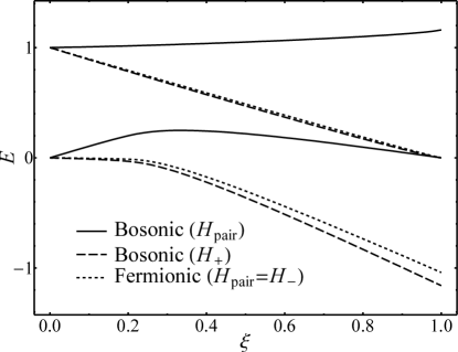
Figure 3: Lowest and highest eigenvalues, within the $(v_{1}v_{2})=(00)$ subspace, for the bosonic two-level pairing model with repulsive pairing interaction, in the usual form as given by $H_{\text{pair}}$ in (93) (solid curves) and after correction by the $\mathrm{U}(n_{1}+n_{2})$ Casimir offset as given by $H_{+}$ in (94) (dashed curves). These are plotted as functions of the control parameter $\xi$ between the weak-coupling and strong-coupling limits. The eigenvalues for the fermionic two-level pairing model with attractive pairing interaction, as given by $H_{\text{pair}}$ or equivalently by $H_{-}$ in (95), are shown for comparison (dotted curves). All calculations are for $N=50$, with $n_{1}=n_{2}=5$ in the bosonic case and $n_{1}=n_{2}=50$ in the fermionic case (see Fig. 4 for more detailed eigenvalue spectra).

To facilitate direct comparison of the bosonic and fermionic quantum phase transitions, it is helpful to instead construct a Hamiltonian for which the ground state energy follows the same trajectory as a function of $\xi$ in the large $N$ limit, and the eigenvalues span the same range at each of the limits, namely, $[0,1]$ for $\xi=0$ and $[-1,0]$ for $\xi=1$. By the results of Sec. 5, this is accomplished by choosing, for repulsive pairing interaction, the Hamiltonian

$$H_{+}=\frac{(1-\xi)}{N}N_{2}+\frac{\xi}{N^{2}}\Biggl{[}4S_{+}S_{-}-\Biggl{\{}\begin{array}[]{c}N(N+2\Omega-2)\\ N(2\Omega-N+2)\end{array}\Biggr{\}}\Biggr{]},$$ (94)

and, for attractive pairing interaction, the usual Hamiltonian

$$H_{-}=\frac{(1-\xi)}{N}N_{2}-\frac{4\xi}{N^{2}}S_{+}S_{-}.$$ (95)

The $c$-number offset included in the definition of $H_{+}$, which arises as $C_{2}[\mathrm{U}(n_{1}+n_{2})]-\theta N$, is included to achieve the same range of eigenvalues in the strong coupling limit, as well as a similar evolution of ground state energy across the transition (Fig. 3), in the large-$N$ limit, thereby facilitating comparison of the bosonic (repulsive pairing) and fermionic (attractive pairing) quantum phase transition. With inclusion of this offset, $H_{+}$ is equivalent to the generalized multipole transitional Hamiltonian (90) when acting on the $(v_{1}v_{2})=(00)$ subspace of any two-level pairing model, as may be seen from (88). In particular, for the $s$-$b$ models, inclusion of this offset makes $H_{+}$ identical to the conventional multipole form (81) of the transitional Hamiltonian, when acting on the $(v_{1}v_{2})=(00)$ subspace.

The evolution of the eigenvalue spectrum across the transition between weak coupling and strong coupling is shown for representative bosonic and fermionic cases in Fig. 4. Specifically, equal-degeneracy pairing models ($n_{1}=n_{2}\equiv\Omega$) are considered, and the $(v_{1}v_{2})=(00)$ states are shown. Here a sufficiently large total occupancy ($N=50$) is chosen such that the precursors of the phase transitional singularities are readily apparent. Spectra are shown for both bosons [Fig. 4 (left)] and fermions [Fig. 4 (right)], with repulsive [Fig. 4 (top)] and attractive [Fig. 4 (bottom)] interactions. Qualitatively similar spectra in the bosonic and fermionic cases are obtained when level degeneracies for the bosonic calculation ($\Omega=5$) are much less than the occupancy, while the degeneracies for the fermionic calculation ($\Omega=50$) are such as to give half filling. Then the “envelope” of the spectrum (the range of eigenvalues at a given value of the Hamiltonian parameter $\xi$) is essentially identical for the bosonic case with repulsive pairing [Fig. 4 (a)] and the fermionic case with attractive pairing [Fig. 4 (d)], i.e., the interactions signs which yield a ground state quantum phase transition. Features to observe include the essentially constant ground state energy for $\xi<1/5$ and downturn [from $0$ to $-1$] for $\xi>1/5$, an approximately linear evolution of the highest eigenvalue from $+1$ to $0$, and a compression of the level density at $E\approx 0$ for $\xi>1/5$, a characteristic of the excited state quantum phase transition [14].

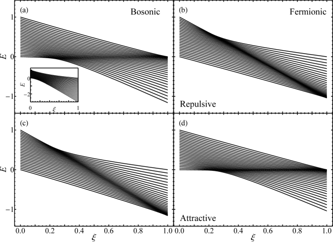
Figure 4: Eigenvalues of the bosonic two-level pairing model, with level degeneracies $n_{1}=n_{2}=5$ (at left), and fermionic two-level pairing model, with level degeneracies $n_{1}=n_{2}=50$ (at right), for repulsive (at top) and attractive (at bottom) pairing interactions, shown for the $(v_{1}v_{2})=(00)$ subspace, as functions of the control parameter $\xi$ between the weak-coupling and strong-coupling limits. All calculations are for $N=50$, thus for $\Omega\ll N$ in the bosonic case and $\Omega=N$ (half filling) in the fermionic case. The alternative regime in which the bosonic system also has $\Omega\approx N$ is shown (specifically, for $n_{1}=n_{2}=51$ and $N=50$) in the inset to panel (a). The Hamiltonians $H_{\pm}$ of (94) and (95) are used in the calculations.

The structure of the eigenvalue spectrum is likewise similar when one compares the bosonic case with attractive pairing [Fig. 4 (c)] and the fermionic case with repulsive pairing [Fig. 4 (b)]. This should hardly be surprising. Indeed, when $n_{1}=n_{2}$, the eigenvalue spectra for Hamiltonians for opposite pairing signs [e.g., Fig. 4 (a) and Fig. 4 (c), or Fig. 4 (b) and Fig. 4 (d)] may be obtained from each other, by negation of the Hamiltonian and interchange of the level labels 1 and 2, to within addition of a $c$-number function of $\xi$. Therefore, in the present example, the resemblance between Fig. 4 (c) and Fig. 4 (b) is a necessary consequence of the resemblance between Fig. 4 (a) and Fig. 4 (d).

The emergence of finite-size precursors to the infinite-$N$ singularities associated with the quantum phase transition depends not only on $N$ but also on the level degeneracies $n_{1}$ and $n_{2}$. An important distinction therefore arises between bosonic and fermionic models [14]. For fermionic systems, the total occupancy $N$ is limited to $n_{1}+n_{2}$. Therefore, the limit of large $N$ can only be taken if the level degeneracies are simultaneously increased. Since at full filling ($N=n_{1}+n_{2}$) the spectrum, like that for zero filling, is trivial, it is more informative to take the limit $N\rightarrow\infty$ at or near half filling [$N={{\textstyle\frac{1}{2}}}(n_{1}+n_{2})\equiv\Omega$]. However, no such restriction arises for bosonic systems, and $N\rightarrow\infty$ can be obtained even for fixed level degeneracies.

Indeed, for the bosonic two-level pairing models, we find numerically that the onset of critical phenomena requires $N\gg\Omega$, not $N\approx\Omega$. The evolution of eigenvalues for the bosonic system with the same occupancy ($N=50$) as in Fig. 4(a), but with level degeneracies comparable to the occupation $n_{1}=n_{2}(=\Omega)=49\approx 50$, analogous to “half filling”, is shown for comparison in Fig. 4 (inset). The eigenvalue spectrum is qualitatively different, as compared to Fig. 4(a) or (d), with respect to each of the properties noted above, e.g., the ground state eigenvalue is not recognizably constant for $\xi<1/5$, there is no apparent change in curvature at $\xi=1/5$, and closer inspection reveals no level spacing compression of the type associated with the excited state quantum phase transition. This is already anticipated from the different eigenvalue range ($\sim 3N^{2}$) in the strong coupling limit, obtained in Sec. 5.5.

Similar distinctions between the large-$N$ limit taken with $N\gg\Omega$ or $N\sim\Omega$ are obtained for the critical scaling properties, which we defer to a more comprehensive study. For now, we restrict attention to the basic energy spectra obtained with the present transitional Hamiltonian for the general two-level pairing model, and note that the spectrum for finite $N$ depends strongly not just on the total degeneracy $n=n_{1}+n_{2}$ of the two levels but on the equality or degree of inequality of the two level degeneracies $n_{1}$ and $n_{2}$.

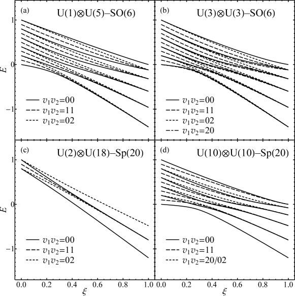
Figure 5: Eigenvalues for the bosonic two-level pairing model, with level degeneracies (a) $n_{1}=1$ and $n_{2}=5$ or (b) $n_{1}=3$ and $n_{2}=3$, and for the fermionic two-level pairing model, with level degeneracies (c) $n_{1}=2$ and $n_{2}=18$ or (d) $n_{1}=10$ and $n_{2}=10$, as functions of the control parameter $\xi$ between the weak-coupling and strong-coupling limits. All calculations are for $N=10$. Eigenvalues are shown only for the lowest-seniority subspaces $(v_{1}v_{2})$, specifically, those with $v_{1}+v_{2}\leq 2$. The Hamiltonian $H_{+}$ of (94) is used for the bosonic calculations and $H_{-}$ of (95) for the fermionic calculations.

The transitional spectra for two different bosonic models with total degeneracy $n=6$, and taken with $N=10$ (i.e., occupation substantially greater than the degeneracy), are compared in Fig. 5 (top): the $s$-$b$ model ($n_{1}=1$ and $n_{2}=5$) [Fig. 5(a)] and the choice of two levels with equal degeneracies ($n_{1}=3$ and $n_{2}=3$) [Fig. 5(b)]. The transitional spectra for the $(v_{1}v_{2})=(00)$ subspaces in Figs. 5(a) and (b) are similar to each other. Although only irreps of type $(0v_{2})$ or $(1v_{2})$ are obtained in the former case, more general irreps $(v_{1}v_{2})$ are possible in the latter case, naturally leading to a more complicated spectrum. In particular, it should be noted that the lowest state from each subspace of the form $(v_{1}0)$ approximately tracks the lowest $(00)$ state in energy, and that these states are in fact lower in energy than the $(00)$ state everywhere between the dynamical symmetry limits [see the lowest curve for $(v_{1}v_{2})=(20)$ in Fig. 5(b)]. It is perhaps not surprising that, given a repulsive pairing interaction, the energy may be lowered by breaking pairs within the lower single-particle energy (i.e., increasing $v_{1}$). In contrast, increasing $v_{2}$ also enforces nonzero occupation ($N_{2}\geq v_{2}$) of the higher single-particle energy level and is therefore not as energetically prefered.

For the fermionic system, the difference between the transitional spectra for near-equal versus highly-imbalanced degeneracies for the two levels is marked. The transitional spectra for two different fermionic models with total degeneracy $n=20$, again taken with $N=10$ (which now represents half filling), are compared in Fig. 5 (bottom): for the most extremely imbalanced possible choice of degeneracies ($n_{1}=2$ and $n_{2}=18$) [Fig. 5(c)] and with equal degeneracies ($n_{1}=10$ and $n_{2}=10$) [Fig. 5(d)]. The quantum phase transition which occurs for equal degeneracies is washed out in the limit of imbalanced degeneracies, as is evident in the simple, near-linear evolution of the ground state energy across Fig. 5(c). Such an effect may be expected on the basis of the Pauli principle. The lower level, of degeneracy $n_{1}=2$, easily saturates at full occupancy, so that the dynamics are effectively those of a one-level system of degeneracy $n_{2}=18$, which does not support critical phenomena as a function of pairing interaction strength.

7 Conclusion

Although the existence of duality relations between the number-conserving unitary and number-nonconserving quasispin algebras for the two-level system with pairing interactions is well known, and indeed these relations have proven useful in practical calculations for specific special cases of the two-level pairing model, here we have sought to establish a systematic treatment of the duality relations, both for bosonic and fermionic two-level pairing models and for arbitrary choice of level degeneracies. A principal goal has been to clarify the relationships between the disparate forms of the Hamiltonian encountered in the study and application of these models. The results are intended to provide a foundation for a more comprehensive investigation of quantum phase transitions in two-level pairing models — including the dependence of scaling properties on the bosonic or fermionic nature of the system and on the level degeneracies — beyond the special cases conventionally considered, namely, bosonic $s$-$b$ models and fermionic models with equal degeneracy. The duality between orthogonal or symplectic algebras and the quasispin algebras is also relevant to the analysis of the classical dynamics of the system, through the associated coset spaces [41]. The dual algebras yield complementary descriptions involving classical coordinate spaces with different dimensionalities [42]. Finally, although the present derivations were given for the case of two-level models, they may readily be extended to the $\mathrm{SO}(n_{1}+n_{2}+\cdots)$ or $\mathrm{Sp}(n_{1}+n_{2}+\cdots)$ algebras associated with multi-level systems, with generators directly generalizing those of (18) and (19), for which the quantum phase transitions have been much less completely studied. Physical realizations of interest in this more general case include the nuclear shell model and descriptions of superconductivity in metallic grains.

Appendix Appendix Spherical tensor commutation relations

When working with angular momentum coupled products of spherical tensor operators, it is convenient to consider the coupled commutator [72, 57], itself a spherical tensor operator, with components given by

$$[A^{(a)},B^{(b)}]^{(c)}_{\gamma}=\sum_{\alpha\beta}(a\alpha b\beta|c\gamma)[A^{(a)}_{\alpha},B^{(b)}_{\beta}].$$ (96)

To clearly set out the identities used in establishing the commutators of the generators in Tables 4 and 5, the basic definitions and properties are summarized in this appendix. The use of coupled commutation results bypasses the tedious process of uncoupling the operators, i.e., introducing multiple sums over products of Clebsch-Gordan coefficients, taking commutators of the spherical tensor components, and then recoupling.

If both bosonic and fermionic operators are to be considered, a consistent set of definitions is obtained if the quantity in brackets is taken to be the graded commutator, that is, either the commutator or the anticommutator according to the bosonic or fermionic nature of the operators. Specifically,

$$[A^{(a)}_{\alpha},B^{(b)}_{\beta}]=A^{(a)}_{\alpha}B^{(b)}_{\beta}-\theta_{ab}B^{(b)}_{\beta}A^{(a)}_{\alpha},$$ (97)

where $\theta_{ab}=+$ if either $A$ or $B$ is a bosonic operator, and $\theta_{ab}=-$ if both $A$ and $B$ are fermionic operators. (For the sake of these definitions, it is assumed that a bosonic operator has integer angular momentum and a fermionic operator has half-integer angular momentum.) The coupled commutator can be written directly in terms of coupled products as

$$[A^{(a)},B^{(b)}]^{(c)}=(A^{(a)}\times B^{(b)})^{(c)}-\theta_{ab}(-)^{c-a-b}(B^{(b)}\times A^{(a)})^{(c)}$$ (98)

and obeys the symmetry or antisymmetry relation

$$[B^{(b)},A^{(a)}]^{(c)}=-\theta_{ab}(-)^{c-a-b}[A^{(a)},B^{(b)}]^{(c)}.$$ (99)

The uncoupled commutators of the spherical tensor components may be recovered from the coupled commutators, if needed, by inverting (96) to give

$$[A^{(a)}_{\alpha},B^{(b)}_{\beta}]=\sum_{c\gamma}(a\alpha b\beta|c\gamma)[A^{(a)},B^{(b)}]^{(c)}_{\gamma}.$$ (100)

The product rule for coupled commutators is [57, (6)]

$$[(A\times B)^{(e)},C]^{(d)}=\sum_{f}\hat{e}\hat{f}\bigl{[}(-)^{a+b+c+d}{\scriptstyle\scriptsize\left\{\begin{array}[]{ccc}a&b&e\\ c&d&f\end{array}\right\}}(A\times[B,C]^{(f)})^{(d)}\@eqncr+\theta_{bc}{\scriptstyle\scriptsize\left\{\begin{array}[]{ccc}a&b&e\\ d&c&f\end{array}\right\}}([A,C]^{(f)}\times B)^{(d)}\bigr{]}.$$ (105)

A second application of this identity yields the double product rule needed for evaluating commutators of one-body or pair operators,

$$[(A\times B)^{(e)},(C\times D)^{(f)}]^{(g)}\@eqncr\qquad=\sum_{hk}\hat{e}\hat{f}\hat{h}\hat{k}\bigl{[}(-)^{e+c+d+g}(-)^{a+b+c+h}{\scriptstyle\scriptsize\left\{\begin{array}[]{ccc}c&d&f\\ g&e&h\end{array}\right\}}{\scriptstyle\scriptsize\left\{\begin{array}[]{ccc}a&b&e\\ c&h&k\end{array}\right\}}[(A\times[B,C]^{(k)})^{(h)}\times D]^{(g)}\@eqncr\qquad+\theta_{bc}(-)^{e+c+d+g}(-)^{b+c+e+k}{\scriptstyle\scriptsize\left\{\begin{array}[]{ccc}c&d&f\\ g&e&h\end{array}\right\}}{\scriptstyle\scriptsize\left\{\begin{array}[]{ccc}a&b&e\\ h&c&k\end{array}\right\}}[([A,C]^{(k)}\times B)^{(h)}\times D]^{(g)}\@eqncr\qquad+\theta_{ec}(-)^{e+c+f+h}(-)^{a+b+d+h}{\scriptstyle\scriptsize\left\{\begin{array}[]{ccc}c&d&f\\ e&g&h\end{array}\right\}}{\scriptstyle\scriptsize\left\{\begin{array}[]{ccc}a&b&e\\ d&h&k\end{array}\right\}}[C\times(A\times[B,D]^{(k)})^{(h)}]^{(g)}\@eqncr\qquad+\theta_{ec}\theta_{bd}(-)^{e+c+f+h}(-)^{b+d+e+k}{\scriptstyle\scriptsize\left\{\begin{array}[]{ccc}c&d&f\\ e&g&h\end{array}\right\}}{\scriptstyle\scriptsize\left\{\begin{array}[]{ccc}a&b&e\\ h&d&k\end{array}\right\}}[C\times([A,D]^{(k)}\times B)^{(h)}]^{(g)}\bigr{]}.$$ (122)

If operators $A^{\dagger}$ and $B^{\dagger}$ are creation operators, obeying cannonical commutation or anticommutation relations, the canonical commutators are represented in coupled form by [57, (10)]

$$[\tilde{A},B^{\dagger}]^{(c)}=\hat{a}\delta_{AB}\delta_{c0}$$ (123)

and $[\tilde{A},\tilde{B}]^{(c)}=[A^{\dagger},B^{\dagger}]^{(c)}=0$. The coupled commutator of two one-body operators is therefore

$$[(A^{\dagger}\times\tilde{B})^{(e)},(C^{\dagger}\times\tilde{D})^{(f)}]^{(g)}=(-)^{2b}(-)^{a+d+g}\hat{e}\hat{f}{\scriptstyle\scriptsize\left\{\begin{array}[]{ccc}e&f&g\\ d&a&b\end{array}\right\}}(A^{\dagger}\times\tilde{D})^{(g)}\delta_{BC}\@eqncr-\theta_{ab}\theta_{bc}\theta_{ca}(-)^{b+c+e+f}\hat{e}\hat{f}{\scriptstyle\scriptsize\left\{\begin{array}[]{ccc}e&f&g\\ c&b&a\end{array}\right\}}(C^{\dagger}\times\tilde{B})^{(g)}\delta_{AD},$$ (128)

as needed, e.g., for the commutators of the generators of $\mathrm{U}(n_{1}+n_{2})$.

References

References

- [1] Botet R and Jullien R 1983 Phys. Rev. B 28 3955
- [2] Rowe D J, Turner P S and Rosensteel G 2004 Phys. Rev. Lett. 93 232502
- [3] Dusuel S and Vidal J 2004 Phys. Rev. Lett. 93 237204
- [4] Dusuel S and Vidal J 2005 Phys. Rev. B 71 224420
- [5] Dusuel S and Vidal J 2005 Phys. Rev. A 71 060304
- [6] Dusuel S, Vidal J, Arias J M, Dukelsky J and García-Ramos J E 2005 Phys. Rev. C 72 011301(R)
- [7] Dusuel S, Vidal J, Arias J M, Dukelsky J and García-Ramos J E 2005 Phys. Rev. C 72 064332
- [8] Leyvraz F and Heiss W D 2005 Phys. Rev. Lett. 95 050402
- [9] Högaasen-Feldman J 1961 Nucl. Phys. 28 258
- [10] Broglia R A, Riedel C and Sørensen B 1968 Nucl. Phys. A 107 1
- [11] Bès D R, Broglia R A, Perazzo R P J and Kumar K 1970 Nucl. Phys. A 143 1
- [12] Cejnar P, Macek M, Heinze S, Jolie J and Dobeš J 2006 J. Phys. A 39 L515
- [13] Heinze S, Cejnar P, Jolie J and Macek M 2006 Phys. Rev. C 73 014306
- [14] Caprio M A, Cejnar P and Iachello F 2008 Ann. Phys. (N.Y.) 323 1106
- [15] Iachello F and Caprio M A 2010 Quantum phase transitions in nuclei Understanding Quantum Phase Transitions ed Carr L D (Boca Raton, FL: CRC Press) chap 27
- [16] Sumaryada T and Volya A 2007 Phys. Rev. C 76 024319
- [17] Pérez-Fernández P, Relaño A, Arias J M, Dukelsky J and García-Ramos J E 2009 Phys. Rev. A 80 032111
- [18] Rowe D J 2004 Phys. Rev. Lett. 93 122502
- [19] Arias J M, Dukelsky J, García-Ramos J E and Vidal J 2007 Phys. Rev. C 75 014301
- [20] von Delft J and Ralph D C 2001 Phys. Rep. 345 61
- [21] de-Shalit A and Talmi I 1963 Nuclear Shell Theory (Pure and Applied Physics no 14) (New York: Academic)
- [22] Iachello F and Arima A 1987 The Interacting Boson Model (Cambridge: Cambridge University Press)
- [23] Law C, Pu H and Bigelow N 1998 Phys. Rev. Lett. 81 5257
- [24] Uchino S, Ostuka T and Ueda M 2008 Phys. Rev. A 78 023609
- [25] Kerman A K 1961 Ann. Phys. (N.Y.) 12 300
- [26] Helmers K 1961 Nucl. Phys. 23 594
- [27] Judd B R 1968 Group theory in atomic spectroscopy Group Theory and Its Applications ed Loebl E M (New York: Academic Press) p 183
- [28] Moshinsky M and Quesne C 1970 J. Math. Phys. 11 1631
- [29] Wybourne B G 1974 Classical Groups for Physicists (New York: Wiley)
- [30] Rowe D J and Wood J L 2010 Fundamentals of Nuclear Models: Foundational Models (Singapore: World Scientific)
- [31] Racah G 1949 Phys. Rev. 76 1352
- [32] Racah G 1965 Springer Tracts Mod. Phys. 37 28
- [33] Kerman A K, Lawson R D and Macfarlane M H 1961 Phys. Rev. 124 162
- [34] Ui H 1968 Ann. Phys. (N.Y.) 49 69
- [35] Lawson R D and Macfarlane M H 1965 Nucl. Phys. 66 80
- [36] Macfarlane M H 1966 Shell model theory of identical nucleons Nuclear Structure Physics (Lectures in Theoretical Physics vol VIII C) ed Kunz P, Lind D A and Brittin W E (Boulder: Univ. of Colorado Press) p 583
- [37] Arima A and Ichimura M 1966 Prog. Theor. Phys. 36 296
- [38] Arima A and Iachello F 1979 Ann. Phys. (N.Y.) 123 468
- [39] Feng Pan and Draayer J P 1998 Nucl. Phys. A 636 156
- [40] Volya A, Brown B A and Zelevinsky V 2001 Phys. Lett. B 509 37
- [41] Gilmore R 1974 Lie Groups, Lie Algebras, and Some of Their Applications (New York: Wiley)
- [42] Feng D H, Gilmore R and Deans S R 1981 Phys. Rev. C 23 1254
- [43] Iachello F 2006 Lie Algebras and Applications (Lecture Notes in Physics vol 708) (Berlin: Springer)
- [44] Lipkin H J, Meshkov N and Glick A J 1965 Nucl. Phys. 62 188
- [45] Hammermesh M 1962 Group Theory and Its Application to Physical Problems (Reading, MA: Addison-Wesley)
- [46] Judd B R 1963 Operator Techniques in Atomic Spectroscopy (New York: McGraw-Hill)
- [47] Gheorghe A and Răduţă A A 2004 J. Phys. A 37 10951
- [48] Gel’fand I M and Cetlin M L 1950 Dokl. Akad. Nauk SSSR 71 1017
- [49] Hecht K T 1965 Nucl. Phys. 63 177
- [50] Kemmer N, Pursey D L and Williams S A 1968 J. Math. Phys. 9 1224
- [51] Caprio M A, Sviratcheva K D and McCoy A E 2010 J. Math. Phys. 51 093518
- [52] Varshalovich D A, Moskalev A N and Khersonskii V K 1988 Quantum Theory of Angular Momentum (Singapore: World Scientific)
- [53] Van Isacker P, Frank A and Dukelsky J 1985 Phys. Rev. C 31 671
- [54] Leviatan A 1987 Ann. Phys. (N.Y.) 179 201
- [55] Nwachuku C O and Rashid M A 1977 J. Math. Phys. 18 1387
- [56] Caprio M A and Iachello F 2007 Nucl. Phys. A 781 26
- [57] Chen J Q, Chen B Q and Klein A 1993 Nucl. Phys. A 554 61
- [58] Lipkin H J 1966 Lie Groups for Pedestrians 2nd ed (Amsterdam: North-Holland)
- [59] Ortiz G, Somma R, Dukelsky J and Rombouts S 2005 Nucl. Phys. B 707 421
- [60] Balantekin A B, de Jesus J H and Pehlivan Y 2007 Phys. Rev. C 75 064304
- [61] Pan F, Xie M X, Guan X, Dai L R and Draayer J P 2009 Phys. Rev. C 80 044306
- [62] Chen H, Brownstein J R and Rowe D J 1990 Phys. Rev. C 42 1422
- [63] Vidal J, Arias J M, Dukelsky J and Garcá-Ramos J E 2006 Phys. Rev. C 73 054305
- [64] Lipas P O, Toivonen P and Warner D D 1985 Phys. Lett. B 155 295
- [65] Iachello F, Zamfir N V and Casten R F 1998 Phys. Rev. Lett. 81 1191
- [66] Somma R, Ortiz G, Barnum H, Knill E and Viola L 2004 Phys. Rev. A 70 042311
- [67] Tsue Y, Providência C, da Providência J and Yamamura M 2007 Prog. Theor. Phys. 117 431
- [68] Gilmore R and Feng D H 1978 Nucl. Phys. A 301 189
- [69] Dieperink A E L, Scholten O and Iachello F 1980 Phys. Rev. Lett. 44 1747
- [70] Ginocchio J N and Kirson M W 1980 Nucl. Phys. A 350 31
- [71] Cejnar P and Iachello F 2007 J. Phys. A 40 581
- [72] French J B 1966 Multipole and sum-rule methods in spectroscopy Proceedings of the International School of Physics “Enrico Fermi”, Course XXXVI ed Bloch C (New York: Academic Press) p 278