Dynamical current-current susceptibility of gapped graphene

Abstract

We present analytical expressions for the current-current correlation function in graphene for arbitrary frequency, wave vector, doping, and band gap induced by a mass term. In the static limit we analyze the Landau (orbital) and Pauli magnetization, as well as the Lindhard correction which describes Friedel and Ruderman-Kittel-Kasuya-Yosida oscillations. In the nonrelativistic limit we compare our results with the situation of the usual two-dimensional electron gas (2DEG). We find that the orbital magnetic susceptibility (OMS) in gapped graphene is smeared out on an energy scale given by the inverse mass. The nonrelativistic limit of the plasmon dispersion and the Lindhard function reproduces the results of the 2DEG. The same conclusion is true for the Pauli part of the susceptibility. The peculiar band structure of gapped graphene leads to pseudospin paramagnetism and thus to a special form of the OMS.

I Introduction

Graphene, which was first isolated in 2004,Novoselov is the name of a monolayer of carbon atoms that are arranged in a hexagonal lattice. It differs compared to most two-dimensional systems by its relativistic energy-momentum relation and its nontrivial spinor structure,Wallace originating from the two-atomic Wigner-Seitz cell, and has remarkable electronic properties.Netro_2009 As a consequence, various effects like the anomalous quantum Hall effect Novoselov2 ; Zhang or the Klein tunneling Young have been discovered. In 1956, the orbital magnetization of two-dimensional graphite had already been calculated, McClure indicating a strong diamagnetism in the undoped hexagonal lattice which was confirmed by recent experiments.Sepioni_2010

In the present work, we study the response of the system to an electromagnetic potential in terms of the current-current correlation function. Similar studies have already been performed recently regarding the density-density response of masslessWunsch ; Sarma and massfulPyat Dirac fermions, the Hall conductivity in the presence of spin-orbit interactionsDyrdal_2009 ; Ingenhoven_2010 including self-energy and vertex corrections,Sinitsyn_2006 and current-current correlations in the absence of a mass term.Polini ; Stauber Here we will generalize those results to the case of massive quasiparticles by taking into account a mass term which breaks sublattice symmetry, leading to a gap between the valence and the conduction band. It can occur due to different mechanisms, including intrinsic spin-orbit couplingMin ; Kane (with a gap of $24\mu eV$),Gmitra_2009 graphene placed on a suitable substrate ($E_{g}=0.26eV$),Zhou or adsorption of molecules (with a gap of several electron volts).Graphan The current correlator is related to the polarization function, which was discussed earlier.Pyat ; Wunsch ; Sarma Its limiting behavior determines the orbital and the Pauli magnetization, the plasmon spectra, and the screening of electric or magnetic impurities. Without the mass term, the Landau magnetization is infinite for intrinsic graphene (i.e. zero chemical potential, $\mu=0$) and zero for extrinsic graphene ($\mu\neq 0$),Polini ; Stauber ; Ando ; McClure ; Sharapov_2004 while the Pauli part vanishes for the former and is finite for the latter case. As gapped graphene is similar to the two-dimensional electron gas (2DEG), we investigate in the nonrelativistic limit, i.e., the limit of single-particle energies just above the band-gap parameter, and compare our results to that of the 2DEG.Stern

The particular features of the density-density and current-current correlation functions in graphene compared to the standard 2DEG rely on the coupling of the orbital degrees of freedom to the sublattice of pseudospin. On the other hand, semiconductor systems involving coupling to other internal degrees of freedom such as the physical electron spin have also been analyzed recently with similar aspects. As examples, we mention studies of the dielectric function of semiconductor 2DEGs with various types of spin-orbit coupling terms, Pletyukhov06 ; Badalyan09 two-dimensional semiconductor hole systems, Cheng01 and $p$-doped bulk semiconductors. Schliemann Moreover, the dielectric function of graphene taking into account the full honeycomb lattice structure (but not a mass term) was analyzed recently in Ref. Stauber10 . Analytical expressions for the polarizability of graphene with finite width of Landau levels, temperature, and mass term can be found in Ref. Pyat2010 .

This paper is organized as follows. After introducing in Sec. II the model Hamiltonian and pertaining quantities, we present in Sec. III analytical expressions for the longitudinal and transversal current-current correlation function. In Sec. IV, we focus on the static limit and determine the orbital and Pauli magnetization. Moreover, we include many-body effects via random-phase approximation (RPA). In Sec. V, we study the effect of an increasing mass term on typical quantities like the magnetic susceptibility, Friedel oscillations, and the plasmon spectra, and we compare the results to the 2DEG. We close with conclusions in Sec. VI. In Appendix A, one can find details of the calculation of the transversal susceptibility, while Appendix B comments on the relation between current and density response.

II The model

The atoms in graphene are arranged in a honeycomb lattice, where each unit cell contains two carbon atoms. The effective Hamiltonian near the corners of the Brillouin zone K/K’, including a mass gap as well as finite doping, is given by, using standard notation

$$\hat{H}_{0} =\sum\limits_{\boldsymbol{k}}\hat{\Psi}_{\boldsymbol{k}}^{\dagger}\begin{pmatrix}\mu+mv_{F}^{2}&\pi_{x}\mp i\pi_{y}\\ \pi_{x}\pm i\pi_{y}&\mu-mv_{F}^{2}\end{pmatrix}\hat{\Psi}_{\boldsymbol{k}}$$ (1)

where we have introduced an electromagnetic vector potential via $\boldsymbol{\pi}=\hbar\boldsymbol{k}+\boldsymbol{A}$. The upper (lower) sign refers to the point K (K’). The field operator is defined by $\boldsymbol{\hat{\Psi}}_{\boldsymbol{k}}=\begin{pmatrix}\hat{a}_{\boldsymbol{k}}\\ \hat{b}_{\boldsymbol{k}}\end{pmatrix}$, where $\hat{a}_{\boldsymbol{k}}$ and $\hat{b}_{\boldsymbol{k}}$ are the destruction operators of the Bloch states in the two sublattices. Concentrating on the K point [upper sign in Eq. (1)], the eigenvalues and eigenspinors at zero vector potential $\boldsymbol{A}=0$ are given by

$$E_{\pm}(\boldsymbol{k})=\mu\pm\sqrt{\left(\hbar v_{F}k\right)^{2}+\left(mv_{F}^{2}\right)^{2}},$$

$$\left|\chi_{\pm}(\boldsymbol{k})\right\rangle=\frac{1}{\sqrt{2}}\begin{pmatrix}\sqrt{1\pm\frac{mv_{F}}{\sqrt{\left(\hbar k\right)^{2}+\left(mv_{F}\right)^{2}}}}\\ \pm\sqrt{1\mp\frac{mv_{F}}{\sqrt{\left(\hbar k\right)^{2}+\left(mv_{F}\right)^{2}}}}\>\frac{k_{x}+ik_{y}}{k}\end{pmatrix},$$

with $k=\sqrt{k_{x}^{2}+k_{y}^{2}}$. The current operator follows from

$$\boldsymbol{\hat{j}}_{\boldsymbol{q}}=\frac{\delta\hat{H}_{0}}{\delta\boldsymbol{A}}=v_{F}\sum\limits_{\boldsymbol{k},\alpha,\beta}\boldsymbol{\hat{\Psi}}^{\dagger}_{\boldsymbol{k}-\boldsymbol{q},\alpha}\boldsymbol{\hat{\sigma}}_{\alpha\beta}\boldsymbol{\hat{\Psi}}_{\boldsymbol{k},\beta}\;,$$ (2)

where $\boldsymbol{\hat{\sigma}}$ are the Pauli matrices. Equation (2) is, up to $v_{F}$, equal to the pseudospin operator. The electric current can be connected with the vector potential via the correlation function $\chi_{\boldsymbol{j}_{\mu}\boldsymbol{j}_{\nu}}$, defined by the Kubo product Guil

$$\chi_{AB}(\omega)=-\frac{i}{\hbar\mathcal{A}}\int_{0}^{\infty}dt\left\langle\left[\hat{A}(t),\hat{B}(0)\right]\right\rangle_{0}e^{i\omega t}e^{-0t}\;.$$

Our system is rotationally invariant and the current is thus a linear combination of a purely longitudinal and a transversal part ($q=\left|\boldsymbol{q}\right|$):

$$\chi_{\boldsymbol{j}_{\mu}\boldsymbol{j}_{\nu}}(\boldsymbol{q},\omega) =\frac{\boldsymbol{q}_{\mu}\boldsymbol{q}_{\nu}}{q^{2}}\chi_{\boldsymbol{j}\boldsymbol{j}}^{L}(q,\omega)$$

$$\hskip 28.45274pt+\left(\delta_{\mu\nu}-\frac{\boldsymbol{q}_{\mu}\boldsymbol{q}_{\nu}}{q^{2}}\right)\chi_{\boldsymbol{j}\boldsymbol{j}}^{T}(q,\omega)\;.$$

For a noninteracting system, $\chi_{\boldsymbol{j}_{\mu}\boldsymbol{j}_{\nu}}(\boldsymbol{q},\omega)$ is given by

$$\chi_{\boldsymbol{j}_{\mu}\boldsymbol{j}_{\nu}}(\boldsymbol{q},\omega)= -\frac{gv_{F}^{2}}{\mathcal{A}}\sum\limits_{\lambda_{1},\lambda_{2},\boldsymbol{k}}\frac{f(E_{\lambda_{1}}(\boldsymbol{k}))-f(E_{\lambda_{2}}(\boldsymbol{k}+\boldsymbol{q}))}{\hbar\omega+E_{\lambda_{1}}(\boldsymbol{k})-E_{\lambda_{2}}(\boldsymbol{k}+\boldsymbol{q})+i0}$$

$$\times\left\langle\chi_{\lambda_{1}}\left(\boldsymbol{k}\right)\right|\boldsymbol{\hat{\sigma}}_{\nu}\left|\chi_{\lambda_{2}}\left(\boldsymbol{k}+\boldsymbol{q}\right)\right\rangle$$

$$\times\left\langle\chi_{\lambda_{2}}\left(\boldsymbol{k}+\boldsymbol{q}\right)\right|\boldsymbol{\hat{\sigma}}_{\mu}\left|\chi_{\lambda_{1}}\left(\boldsymbol{k}\right)\right\rangle,$$ (3)

where $f(E)$ is the Fermi function, and $g$ counts orbital and spin degeneracies ($g=4$ in graphene).

The orbital magnetic susceptibility is given by the static transversal part of $\chi_{\boldsymbol{j}\boldsymbol{j}}$:Guil

$$\tilde{\chi}_{orb}=\frac{e^{2}}{c^{2}}\lim\limits_{q\to 0}\frac{\chi_{\boldsymbol{j}\boldsymbol{j}}^{T}(q,0)}{q^{2}}\;.$$ (4)

Because of the continuity equation, $i\partial_{t}\hat{\rho}_{\boldsymbol{q}}=\boldsymbol{q}\cdot\boldsymbol{\hat{j}}_{\boldsymbol{q}}$, the response to a scalar potential, i.e., the polarization function, is included in the current-current susceptibility. In graphene, this leads to the following relation (see Appendix B):Polini ; Stauber

$$\omega^{2}\>\chi_{\rho\rho}(q,\omega)=q^{2}\chi_{\boldsymbol{j}\boldsymbol{j}}^{L}(q,\omega)-\frac{1}{\hbar\mathcal{A}}\left\langle\left[\boldsymbol{q}\cdot\boldsymbol{\hat{j}}_{\boldsymbol{q}},\hat{\rho}_{-\boldsymbol{q}}\right]\right\rangle_{0}.$$ (5)

The second term on the right-hand side was calculated in Ref. Sabio and reads

$$\frac{1}{\hbar\mathcal{A}}\left\langle\left[\boldsymbol{q}\cdot\boldsymbol{\hat{j}}_{\boldsymbol{q}},\hat{\rho}_{-\boldsymbol{q}}\right]\right\rangle=\frac{gq^{2}D}{8\pi\hbar^{2}},$$

where $D$ is a cutoff parameter, which is usually chosen to be of the order of the inverse lattice constant.Peres Note that the commutator is independent of the mass.

For the following, it is essential to distinguish the cases $mv_{F}^{2}>\mu$ and $\mu>mv_{F}^{2}$. In the first, intrinsic case, the Fermi energy lies between the two bands, while in the second, extrinsic case, the Fermi energy lies either in the conduction or in the valence band. From here, we will omit the spatial indices and use the notation $\chi_{jj}\equiv\chi_{\boldsymbol{j}_{x}\boldsymbol{j}_{x}}$.

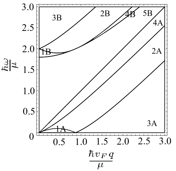
Figure 1: The different regions related to the imaginary part of the current-current correlation function for the extrinsic case of $mv_{F}^{2}/\mu=0.9$. See Table 1 for the definitions of 1A-5B.

Table 1: Definition of the different regions in the $q$-$\omega$-plane related to the imaginary part of the current-current correlation function in the extrinsic case, cf. Eq.(9).

1A:	$\hbar\omega<\mu-\sqrt{(\hbar v_{F})^{2}(q-k_{F})^{2}+(mv_{F}^{2})^{2}}$
1B:	$q<2k_{F}\wedge\;\sqrt{(\hbar v_{F}q)^{2}+4(mv_{F}^{2})^{2}}<\hbar\omega$
	$\hskip 22.76228pt<\mu+\sqrt{(\hbar v_{F})^{2}(q-k_{F})^{2}+(mv_{F}^{2})^{2}}$
2A:	$\pm\mu\mp\sqrt{(\hbar v_{F})^{2}(q-k_{F})^{2}+(mv_{F}^{2})^{2}}<\hbar\omega$
	$\hskip 22.76228pt<-\mu+\sqrt{(\hbar v_{F})^{2}(q+k_{F})^{2}+(mv_{F}^{2})^{2}}$
2B:	$\mu+\sqrt{(\hbar v_{F})^{2}(q-k_{F})^{2}+(mv_{F}^{2})^{2}}<\hbar\omega$
	$\hskip 22.76228pt<\mu+\sqrt{(\hbar v_{F})^{2}(q+k_{F})^{2}+(mv_{F}^{2})^{2}}$
3A:	$\hbar\omega<-\mu+\sqrt{(\hbar v_{F})^{2}(q-k_{F})^{2}+(mv_{F}^{2})^{2}}$
3B:	$\hbar\omega>\mu+\sqrt{(\hbar v_{F})^{2}(q+k_{F})^{2}+(mv_{F}^{2})^{2}}$
4A:	$-\mu+\sqrt{(\hbar v_{F})^{2}(q+k_{F})^{2}+(mv_{F}^{2})^{2}}<\hbar\omega$
	$\hskip 22.76228pt<\hbar v_{F}q$
4B:	$q>2k_{F}\;\wedge\;\sqrt{(\hbar v_{F}q)^{2}+4(mv_{F}^{2})^{2}}<\hbar\omega$
	$\hskip 22.76228pt<\mu+\sqrt{(\hbar v_{F})^{2}(q-k_{F})^{2}+(mv_{F}^{2})^{2}}$
5B:	$\hbar v_{F}q<\hbar\omega<\sqrt{(\hbar v_{F}q)^{2}+4(mv_{F}^{2})^{2}}$

III Results

We restrict our discussions without loss of generality to positive frequencies $\omega$, chemical potentials $\mu$, and mass $m$. All other cases follow from $\chi^{T/L}_{jj}(q,-\omega)=\left[\chi^{T/L}_{jj}(q,\omega)\right]^{*}$ and by observing that the results only depend on the absolute value of $\mu$ and $m^{2}$.

III.1 Intrinsic case

In the intrinsic case, only transitions from the valence into the conduction band contribute. As described in the last section, the longitudinal part, i.e., $\boldsymbol{q}=q\boldsymbol{\hat{x}}$, can be obtained from (5) and the density response given in Ref. Pyat . The longitudinal part was also directly calculated by the authors in order to check relation (5) for finite $m$. Because of the similarity to the transversal case, we restrict details of the calculation, given in the appendix, to the latter. The results are:

$$\operatorname{Im}\left\{\chi_{jj}^{L/T,int}\left(q,\omega\right)\right\}=\frac{g\omega}{16\hbar}\sqrt{1-\left(\frac{v_{F}q}{\omega}\right)^{2}}^{\,\mp 1}\left(1+\frac{\left(2mv_{F}^{2}\right)^{2}}{\hbar^{2}\left(\omega^{2}-(v_{F}q)^{2}\right)}\right)\theta\left((\hbar\omega)^{2}-\left(\hbar v_{F}q\right)^{2}-\left(2mv_{F}^{2}\right)^{2}\right),$$ (6)

$$\operatorname{Re}\left\{\chi_{jj}^{L,int}\left(q,\omega\right)\right\}=\frac{g\left(D-2mv_{F}^{2}\right)}{8\pi\hbar^{2}}+\frac{gmv_{F}^{2}q^{2}}{4\pi\hbar^{2}\left(q^{2}-\omega^{2}/v_{F}^{2}\right)}+\frac{g\omega^{2}}{8\pi\hbar\sqrt{\left|(v_{F}q)^{2}-\omega^{2}\right|}}\left(1+\frac{\left(2mv_{F}^{2}\right)^{2}}{\hbar^{2}\left(\omega^{2}-(v_{F}q)^{2}\right)}\right)$$

$$\hskip 28.45274pt\times\left[\theta\left(v_{F}q-\omega\right)\operatorname{arccos}\left(\frac{2mv_{F}^{2}}{\sqrt{\left(2mv_{F}^{2}\right)^{2}+\hbar^{2}\left((v_{F}q)^{2}-\omega^{2}\right)}}\right)-\theta\left(\omega-v_{F}q\right)\operatorname{arctanh}\left(\frac{2mv_{F}^{2}}{\hbar\sqrt{\omega^{2}-(v_{F}q)^{2}}}\right)\right],$$ (7)

$$\operatorname{Re}\left\{\chi_{jj}^{T,int}\left(q,\omega\right)\right\}=\frac{g\left(D-2mv_{F}^{2}\right)}{8\pi\hbar^{2}}-\frac{g\sqrt{\left|(v_{F}q)^{2}-\omega^{2}\right|}}{8\pi\hbar}\left(1+\frac{\left(2mv_{F}^{2}\right)^{2}}{\hbar^{2}\left(\omega^{2}-(v_{F}q)^{2}\right)}\right)$$

$$\hskip 28.45274pt\times\left[\theta\left(v_{F}q-\omega\right)\operatorname{arccos}\left(\frac{2mv_{F}^{2}}{\sqrt{\left(2mv_{F}^{2}\right)^{2}+\hbar^{2}\left((v_{F}q)^{2}-\omega^{2}\right)}}\right)-\theta\left(\omega-v_{F}q\right)\operatorname{arctanh}\left(\frac{2mv_{F}^{2}}{\hbar\sqrt{\omega^{2}-(v_{F}q)^{2}}}\right)\right],$$ (8)

where $\theta\left(x\right)$ denotes the Heaviside step function.

III.2 Extrinsic case

We have two contributions for the extrinsic case. The first one is the undoped part where only interband transitions contribute (see above), while the second takes into account intraband transitions. Like in the intrinsic case, the longitudinal part is related to the density-density susceptibility via (5):

$$\operatorname{Im}\left\{\chi_{jj}^{L/T,ext}\left(q,\omega\right)\right\}=\frac{g\omega}{16\pi\hbar}\sqrt{\left|1-\left(\frac{v_{F}q}{\omega}\right)^{2}\right|}^{\,\mp 1}\begin{cases}G_{>}^{\mp}\left(\frac{2\mu+\hbar\omega}{\hbar v_{F}q}\right)-G_{>}^{\mp}\left(\frac{2\mu-\hbar\omega}{\hbar v_{F}q}\right)&\text{1A}\\ 0&\text{1B}\\ G_{>}^{\mp}\left(\frac{2\mu+\hbar\omega}{\hbar v_{F}q}\right)&\text{2A}\\ \mp G_{<}^{\mp}\left(\frac{2\mu-\hbar\omega}{\hbar v_{F}q}\right)&\text{2B}\\ 0&\text{3A}\\ \pi\left(1+\frac{\left(2mv_{F}^{2}\right)^{2}}{\hbar^{2}\left(\omega^{2}-(v_{F}q)\right)^{2}}\right)&\text{3B}\\ 0&\text{4A}\\ \pi\left(1+\frac{\left(2mv_{F}^{2}\right)^{2}}{\hbar^{2}\left(\omega^{2}-(v_{F}q)\right)^{2}}\right)&\text{4B}\\ 0&\text{5B ,}\end{cases}$$ (9)

$$\operatorname{Re}\left\{\chi_{jj}^{L/T,ext}\left(q,\omega\right)\right\}=\frac{gD}{8\pi\hbar^{2}}\pm\frac{g\mu\omega^{2}}{2\pi\left(\hbar v_{F}q\right)^{2}}\mp\frac{g\omega}{16\pi\hbar}\sqrt{\left|1-\left(\frac{v_{F}q}{\omega}\right)^{2}\right|}^{\,\mp 1}\,\begin{cases}0&\text{1A}\\ G_{>}^{\mp}\left(\frac{2\mu+\hbar\omega}{\hbar v_{F}q}\right)-G_{>}^{\mp}\left(\frac{2\mu-\hbar\omega}{\hbar v_{F}q}\right)&\text{1B}\\ \pm G_{<}^{\mp}\left(\frac{2\mu-\hbar\omega}{\hbar v_{F}q}\right)&\text{2A}\\ G_{>}^{\mp}\left(\frac{2\mu+\hbar\omega}{\hbar v_{F}q}\right)&\text{2B}\\ \pm G_{<}^{\mp}\left(\frac{2\mu-\hbar\omega}{\hbar v_{F}q}\right)\pm G_{<}^{\mp}\left(\frac{2\mu+\hbar\omega}{\hbar v_{F}q}\right)&\text{3A}\\ G_{>}^{\mp}\left(\frac{2\mu+\hbar\omega}{\hbar v_{F}q}\right)-G_{>}^{\mp}\left(\frac{-2\mu+\hbar\omega}{\hbar v_{F}q}\right)&\text{3B}\\ \pm G_{<}^{\mp}\left(\frac{2\mu-\hbar\omega}{\hbar v_{F}q}\right)\mp G_{<}^{\mp}\left(\frac{2\mu+\hbar\omega}{\hbar v_{F}q}\right)&\text{4A}\\ G_{>}^{\mp}\left(\frac{2\mu+\hbar\omega}{\hbar v_{F}q}\right)+G_{>}^{\mp}\left(\frac{-2\mu+\hbar\omega}{\hbar v_{F}q}\right)&\text{4B}\\ G_{0}^{\mp}\left(\frac{2\mu+\hbar\omega}{\hbar v_{F}q}\right)-G_{0}^{\mp}\left(\frac{2\mu-\hbar\omega}{\hbar v_{F}q}\right)&\text{5B .}\end{cases}$$ (10)

Here we used the shorthand notation

$$G_{<}^{\pm}=x\sqrt{x_{0}^{2}-x^{2}}\pm\left(2-x_{0}^{2}\right)\operatorname{arccos}\left(\frac{x}{x_{0}}\right),$$

$$G_{>}^{\pm}=x\sqrt{x^{2}-x_{0}^{2}}\pm\left(2-x_{0}^{2}\right)\operatorname{arccosh}\left(\frac{x}{x_{0}}\right),$$

$$G_{0}^{\pm}=x\sqrt{x^{2}-x_{0}^{2}}\pm\left(2-x_{0}^{2}\right)\operatorname{arcsinh}\left(\frac{x}{\left|x_{0}\right|}\right),$$

with $x_{0}=\sqrt{1+\frac{\left(2mv_{F}^{2}\right)^{2}}{\hbar^{2}\left((v_{F}q)^{2}-\omega^{2}\right)}}$, and the regions (1A)-(5B), defined in Table 1 and Ref. Pyat . The chemical potential is defined as $\mu=\sqrt{(\hbar v_{F}k_{F})^{2}+(mv_{F}^{2})^{2}}$. The above functions are one of the main results of this work. In the absence of a gap, we recover previous results.Polini ; Stauber Figure 1 illustrates the structure of the regions related to the imaginary part for the specific choice $mv_{F}^{2}/\mu=0.9$.

IV Static limit and magnetic susceptibility

In the static limit, the purely real transversal susceptibility is given by

$$\chi_{jj}^{T,int}\left(q,0\right)=\frac{gD}{8\pi\hbar^{2}}-\frac{gmv_{F}^{2}}{4\pi\hbar^{2}}-\frac{gv_{F}q}{8\pi\hbar}\left(1-\left(\frac{2mv_{F}}{\hbar q}\right)^{2}\right)\operatorname{arccos}\left(\frac{2mv_{F}}{\sqrt{(2mv_{F})^{2}+(\hbar q)^{2}}}\right),$$ (11)

$$\chi_{jj}^{T,ext}\left(q,0\right)=\frac{gD}{8\pi\hbar^{2}}-\frac{gv_{F}q}{8\pi\hbar}\left[\frac{2\mu}{\hbar v_{F}q}\sqrt{1-\left(\frac{2k_{F}}{q}\right)^{2}}+\left(1-\left(\frac{2mv_{F}}{\hbar q}\right)^{2}\right)\cdot\operatorname{arccos}\left(\frac{2\mu}{\hbar v_{F}qx_{0}}\right)\right]\theta\left(q-2k_{F}\right),$$ (12)

while the longitudinal part vanishes, except for the constant term in front. Figure 2 shows the function

$$\frac{1}{q^{2}}\Pi^{T}(q,0)=\frac{1}{q^{2}}\left(\chi_{jj}^{T}\left(q,0\right)-\frac{gD}{8\pi\hbar^{2}}\right)$$

for different values of $a\equiv mv_{F}^{2}/\mu$.

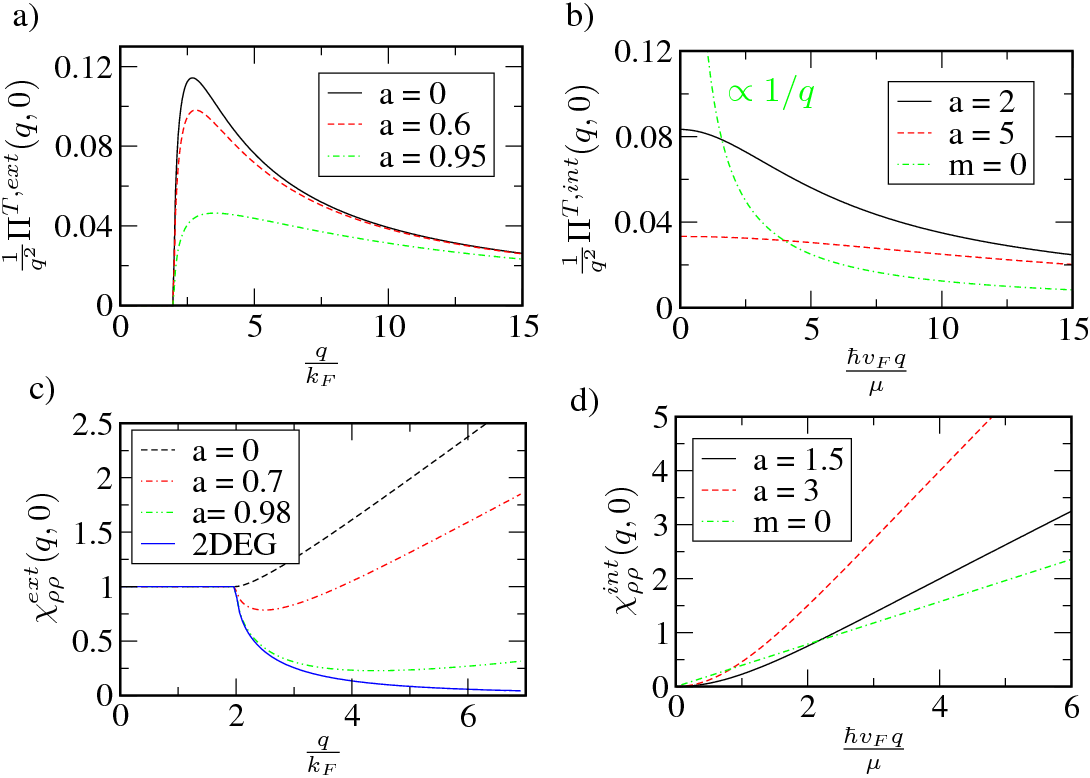
Figure 2: (Color online) Static current correlation function for (a) extrinsic [Eq. (12)] and (b) intrinsic [Eq. (11)] graphene for different ratios $a\equiv mv_{F}^{2}/\mu$ in units of $\frac{-gv_{F}}{2\pi\hbar k_{F}}$. Static polarization for (c) extrinsic [Eq. (16)] and (d) intrinsic [Eq. (15)] graphene in units of $\frac{g\mu}{2\pi\hbar^{2}v_{F}^{2}}$.

We now insert the above functions into (4). The intrinsic part,

$$\tilde{\chi}_{orb}^{int}=-\frac{ge^{2}}{12\pi c^{2}m}\;,$$ (13)

is finite and diamagnetic. Compared to the gapless case, the orbital magnetic susceptibility (OMS) is smeared out on a scale of $1/m$. This broadening of $\tilde{\chi}_{orb}$ also occurs in the presence of disorder,Fukuyama as well as for finite temperature.McClure From (12), one can see that $\Pi^{T,ext}\left(q,0\right)=0$ for $q<2k_{F}$ and thus

$$\tilde{\chi}_{orb}^{ext}=0\;,$$

which is the same as for ungapped graphene. The same result, namely,

$$\tilde{\chi}_{orb}=-\frac{ge^{2}}{12\pi c^{2}m}\>\theta\left(mv_{F}^{2}-\mu\right)\;,$$ (14)

was obtained earlier by energy considerations.Sharapov_2004 ; Ando The limit $m=0$ reproduces previous results:Polini ; Stauber ; McClure

$$\tilde{\chi}_{orb}=-\frac{ge^{2}v_{F}^{2}}{6\pi c^{2}}\delta\left(\mu\right)\;.$$

The expressions for the magnetization given above are only valid for the noninteracting system. A simple way to include many-body effects is via the random-phase approximation.Guil The OMS in RPA is given by

$$\tilde{\chi}_{orb}^{RPA}=\lim\limits_{q\to 0}\frac{\frac{1}{q^{2}}\Pi^{T}(q,0)}{1-\frac{2\pi e^{2}}{\epsilon_{0}q}\Pi^{T}(q,0)}=-\frac{ge^{2}}{12\pi c^{2}m}\theta\left(mv_{F}^{2}-\mu\right),$$

where $\epsilon_{0}$ is the background dielectric constant. One can see that screening effects do not change the Landau part of the magnetization. Without a mass gap, the RPA result

$$\tilde{\chi}_{orb}^{RPA}=\left[1+\frac{g\pi e^{2}}{8\epsilon_{0}}\right]^{-1}\tilde{\chi}_{orb}$$

yields to a renormalization, but the OMS remains infinite and zero, respectively. The situation changes, however, if one includes interaction effects in first-order perturbation theory beyond RPA, leading to paramagnetic behavior in doped graphene sheets.Polini2
The spin correlation function of a noninteracting system equals the density-density susceptibility.Guil The Pauli contribution to the magnetization follows from the limit

$$\tilde{\chi}_{P}=\mu_{B}^{2}\lim\limits_{q\to 0}\chi_{S_{z}S_{z}}(q,0)\;,$$

where $\mu_{B}=\frac{e\hbar}{2m_{0}c}$ is the Bohr magneton and $m_{0}$ is the electrons bare mass. The static polarization readsPyat

$$\chi^{int}_{\rho\rho}(q,0)=\frac{gm}{4\pi\hbar^{2}}-\frac{g\left(\left(\frac{2mv_{F}}{\hbar}\right)^{2}-q^{2}\right)}{8\pi\hbar v_{F}q}\operatorname{arccos}\left(\frac{2mv_{F}}{\sqrt{(2mv_{F})^{2}+(\hbar q)^{2}}}\right),$$ (15)

$$\chi^{ext}_{\rho\rho}\left(q,0\right)=\frac{g\mu}{2\pi\hbar^{2}v_{F}^{2}}\left\{1-\frac{1}{2}\left[\sqrt{1-\left(\frac{2k_{F}}{q}\right)^{2}}-\frac{(\hbar v_{F}q)^{2}-\left(2mv_{F}^{2}\right)^{2}}{2\hbar v_{F}\mu\,q}\operatorname{arccos}\left(\frac{2\mu}{\sqrt{\left(\hbar v_{F}q\right)^{2}+\left(2mv_{F}^{2}\right)^{2}}}\right)\right]\,\theta\left(q-2k_{F}\right)\right\}.$$ (16)

The Pauli part vanishes in the intrinsic case, reflecting the absence of states on the Fermi surface, while the extrinsic part is finite:

$$\tilde{\chi}_{P}=\frac{ge^{2}\mu}{8\pi m_{0}^{2}c^{2}v_{F}^{2}}\>\theta\left(\mu-mv_{F}^{2}\right)\;.$$ (17)

Figure 2 displays the static polarization for different ratios $a=mv_{F}^{2}/\mu$. The limit $a\to 1$ reflects the nonrelativistic case.

V Nonrelativistic limit

V.1 Magnetic susceptibility

The static transversal correlation function for the 2DEG,Guil

$$\chi^{T,2DEG}_{jj}(q,0)=-\frac{gq^{2}}{24\pi m}\left[1-\left(1-\frac{4k_{F}^{2}}{q^{2}}\right)^{3/2}\theta\left(q-2k_{F}\right)\right],$$

leads to the OMS

$$\tilde{\chi}^{2DEG}_{orb}=-\frac{ge^{2}}{24\pi mc^{2}}\;,$$

where $g$ is a degeneracy factor. As described in the last section, the Pauli contribution to the total magnetization is given by the static polarization function Stern

$$\chi_{\rho\rho}^{2DEG}(q,0)=\frac{gm}{2\pi\hbar^{2}}\left[1-\theta\left(q-2k_{F}\right)\sqrt{1-\left(\frac{2k_{F}}{q}\right)^{2}}\;\right],$$

and leads to

$$\tilde{\chi}_{P}^{2DEG}=\mu_{B}^{2}\>\frac{gm}{2\pi\hbar^{2}}=\frac{ge^{2}m}{8\pi m_{0}^{2}c^{2}}\;.$$

Figure 3 displays the function

$$\tilde{\chi}_{tot}^{2DEG}(q,0)=\mu_{B}^{2}\,\chi_{\rho\rho}^{2DEG}(q,0)+\frac{e^{2}}{c^{2}q^{2}}\,\chi^{T,2DEG}_{jj}(q,0)$$

$$=\frac{ge^{2}}{12\pi mc^{2}}\left[1-\frac{3}{2}\theta\left(q-2k_{F}\right)\left\{\sqrt{1-\left(\frac{2k_{F}}{q}\right)^{2}}\right.\right.$$ (18)

$$\left.\hskip 56.9055pt\left.-\frac{1}{3}\left(1-\left(\frac{2k_{F}}{q}\right)^{2}\right)^{3/2}\right\}\right]$$

for the special case $m=m_{0}$. Its limit $q\to 0$ determines the total magnetic susceptibility:

$$\tilde{\chi}_{tot}^{2DEG}=\frac{ge^{2}m}{8\pi c^{2}m_{0}^{2}}\left(1-\frac{1}{3}\left(\frac{m_{0}}{m}\right)^{2}\right)\stackrel{{\scriptstyle m=m_{0}}}{{=}}\frac{ge^{2}}{12\pi c^{2}m}\;.$$ (19)

Figure 3: (Color online) (a) Intraband part of the transversal current correlation function in graphene for different ratios $a\equiv mv_{F}^{2}/\mu$. (b) Sum of Pauli and Landau contribution in the 2DEG for the special case $m=m_{0}$. Both quantities are given in units of $\frac{ge^{2}}{12\pi c^{2}m}$.

Expanding the graphene Hamiltonian (1) in the limit $\pi/mv_{F}\ll 1$, and eliminating the lower spinor component, one finds Ando

$$\hat{H}_{A}=\frac{\boldsymbol{\pi}^{2}}{2m}+\frac{\kappa}{2}g^{*}\mu_{B}B\;,$$ (20)

where $g^{*}=2\frac{m_{0}}{m}$ is the effective Lande factor. $\kappa$ is dependent on the valley, i.e., $\kappa=-1$ for the K point and $\kappa=+1$ for K’. Equation (20) is the well-known Hamiltonian of the 2DEG, including a Zeeman term which changes its sign by interchanging the two valleys. This Zeeman term, however, has nothing to do with the splitting of the energy levels due to the real spin, but is a truly band structure effect. Because of this, the second part of (20) is denoted as the pseudospin Zeeman term.Ando If we neglect states with negative energies, then the susceptibility associated with $\hat{H}_{A}$ is that of (18), while the magnetization is given by (19). At the same time, the OMS of extrinsic graphene, i.e., for $\mu>mv_{F}^{2}$, including only intraband contributions, is given by the paramagnetic term

$$\tilde{\chi}_{orb}^{intraband}=\frac{ge^{2}}{12\pi c^{2}m}\;,$$ (21)

which means that the OMS of gapped graphene without hole states reproduces the total susceptibility of the 2DEG, i.e., the sum of the Pauli and the Landau part. Additionally, (17) describes the Pauli part due to the real spin. In the nonrelativistic limit $\mu\approx mv_{F}^{2}+\frac{\hbar^{2}k_{F}^{2}}{2m}$, Eq. (17) reads

$$\tilde{\chi}_{P}\approx\frac{ge^{2}m}{8\pi c^{2}m_{0}^{2}}\;,$$ (22)

which is just the result of the 2DEG. Note that (22) is true for extrinsic graphene with and without interband contributions.

V.2 Friedel oscillations and plasmon dispersion

Because of the divergent first derivative of the Lindhard correction (i.e., the static polarization) at $q=2k_{F}$ [see Fig. 2(c) for $a>0$], Friedel oscillations in gapped graphene behave differently compared to the gapless case, where the first derivative is finite but the second diverges [see Fig. 2(c) for $a=0$]. The system’s reaction to charged impurities is described by Pyat

$$\Phi_{total}(r) =-\frac{Q\left(m{v_{F}}^{2}\right)^{2}}{\epsilon_{0}a_{0}\mu^{2}}\cdot\frac{\left(2k_{F}\right)^{2}}{\left(2k_{F}+\frac{1}{a_{0}}\right)^{2}}\cdot\frac{\sin{(2k_{F}r)}}{\left(2k_{F}r\right)^{2}},$$

and is similar to the induced spin density $\delta m(r)$, which describes the interaction between magnetic moments, e.g., due to magnetic impurities:

$$\delta m\left(\boldsymbol{r}\,\right) \propto-\int\frac{d\,^{2}q}{\left(2\pi\right)^{2}}\cdot\chi_{\rho\rho}(q,0)\cdot e^{i\boldsymbol{q}\cdot\boldsymbol{r}}$$

$$=\frac{g\left(m{v_{F}}^{2}\right)^{2}\cdot\left(2k_{F}\right)^{2}}{\left(2\pi v_{F}\right)^{2}\hbar\mu}\cdot\frac{\sin{\left(2k_{F}r\right)}}{\left(2k_{F}r\right)^{2}}.$$

Here, $a_{0}=\frac{\epsilon_{0}\hbar^{2}{v_{F}}^{2}}{ge^{2}\mu}$ is an effective Bohr radius. In both cases, the nonrelativistic limit reproduces the result of the 2DEG,Stern

$$\Phi_{total}(r)\approx-\frac{Q}{\epsilon_{0}a_{0}}\cdot\frac{4k_{F}^{2}}{\left(2k_{F}+\frac{1}{a_{0}}\right)^{2}}\cdot\frac{\sin{(2k_{F}r)}}{\left(2k_{F}r\right)^{2}}$$

andBeal

$$\delta m(r)\propto\frac{gm\left(2k_{F}\right)^{2}}{\left(2\pi\right)^{2}\hbar}\cdot\frac{\sin{\left(2k_{F}r\right)}}{\left(2k_{F}r\right)^{2}},$$

while the massless case yields a different power law,Wunsch

$$\Phi_{total}(r)/\delta m\left(\boldsymbol{r}\,\right)\; \propto\frac{\sin{\left(2k_{F}r\right)}}{(k_{F}r)^{3}}.$$

The long wavelength limit of the longitudinal susceptibility determines the dispersion of the collective modes.Guil While plasmons are absent in intrinsic graphene, their dispersion for the extrinsic case reads Pyat

$$\hbar\omega_{p}\left(q\right)=\sqrt{\frac{ge^{2}\mu}{2\epsilon_{0}}\cdot\left[1-\left(\frac{m{v_{F}}^{2}}{\mu}\right)^{2}\right]\cdot q}.$$

In the nonrelativistic limit, this can be approximated as ($n=\frac{g{k_{F}}^{2}}{4\pi}$)

$$\hbar\omega_{p}(q)\approx\sqrt{\frac{2\pi\left(e\hbar\right)^{2}n}{m\epsilon_{0}}\cdot q}$$ (23)

which equals the 2DEG result Stern and particularly shows the same $\sqrt{n}$ density dependence in contrast to the $n^{1/4}$ behavior of $m=0$.Sarma

V.3 Behavior near the threshold $\omega=v_{F}q$

The longitudinal current correlation function for graphene without bandgap is singular at $\omega=v_{F}q$. This solely results from the linear dispersion relation. In gapped graphene, however, the singularity vanishes and the response quantities discussed in this work are smeared out on a scale of $1/m$. This is in accordance with the Lindhard function of the 2DEG,Stern which is not singular at the threshold $\omega=v_{F}q$. However, both the imaginary and the real part of $\chi_{\rho\rho}^{2DEG}$ are finite, while $\operatorname{Im}\left\{\chi_{\rho\rho}(q,v_{F}q)\right\}$ vanishes in graphene [see Eq. (9) for 4A and 5B] and is thus in contrast to the 2DEG result. Furthermore, the real part at $\omega=v_{F}q$ also differs from the result of the 2DEG.

VI Conclusions

In this work, we have derived analytical expressions for the current-current correlation function of graphene for arbitrary frequencies, wave vectors, and doping, including a mass term whose sign depends on the sublattice. The static limit is of particular importance as it determines the magnetization of the system and the screening of impurities. The Landau magnetization of graphene without the mass term is proportional to the $\delta$ function with respect to energy. As we have shown, this changes for finite masses in the intrinsic case, while the extrinsic result remains zero. The Pauli part of the susceptibility was found to be finite and positive for the extrinsic case and zero for the intrinsic case. As gapped graphene is formally quite similar to the 2DEG, we studied the nonrelativistic limit of the magnetization, the Friedel oscillations and the plasmon dispersion. We have demonstrated that all of these quantities, which follow directly from the transversal or longitudinal current correlation function, can reproduce the corresponding 2DEG results (e.g., the $n^{1/2}$ density dependence of the plasmon spectra or the $1/r^{2}$ decay law of the Friedel oscillations), but with one particularity, namely, the pseudospin Zeeman coupling.

Appendix A Details of the calculation of the transversal susceptibility

In this section, we present details of the calculation of the transversal part of the current-current susceptibility. At zero temperature, Eq. (3) can be written as $\chi_{jj}(\boldsymbol{q},\omega)=\xi_{\mu}^{+}+\xi_{\mu}^{-}-\xi_{D}^{-}$ with

$$\xi^{\pm}_{\Lambda}(\boldsymbol{q},\omega)=-\frac{gv_{F}^{2}}{4\pi^{2}} \int\limits d^{2}k\>\frac{1}{2}\left(1\mp\frac{(mv_{F})^{2}-\hbar^{2}k^{2}\left(1-2\sin^{2}\varphi_{\boldsymbol{k}}\right)-\hbar^{2}qk\cos{\left(\varphi_{\boldsymbol{k}}+\varphi_{\boldsymbol{q}}\right)}}{E(k)\cdot E(\boldsymbol{k}+\boldsymbol{q})}\right)\>\theta\left(\Lambda^{2}-(mv_{F}^{2})^{2}-(\hbar v_{F}k)^{2}\right)$$

$$\times\left(\frac{1}{\hbar\omega\mp E(\boldsymbol{k}+\boldsymbol{q})+E(k)+i0}-\frac{1}{\hbar\omega\pm E(\boldsymbol{k}+\boldsymbol{q})-E(k)+i0}\right).$$

The plus (minus) sign corresponds to $\lambda_{1}=\lambda_{2}$ ($\lambda_{1}=-\lambda_{2}$). $\varphi_{\boldsymbol{k}}$ is the angle between $\boldsymbol{k}$ and the $\boldsymbol{\hat{x}}$ axis. For the longitudinal case ($\boldsymbol{q}=q\boldsymbol{\hat{x}}$), we obtain $\cos{\left(\varphi_{\boldsymbol{k}}+\varphi_{\boldsymbol{q}}\right)}=\cos{\varphi_{\boldsymbol{k}}}$, whereas the overlap for the transversal part ($\boldsymbol{q}=q\boldsymbol{\hat{y}}$) is given by $\cos{\left(\varphi_{\boldsymbol{k}}+\pi/2\right)}=-\sin{\varphi_{\boldsymbol{k}}}$. We now set for brevity $\hbar=v_{F}=1$.

A.1 Imaginary part

We define the expression

$$I_{\sigma\tau}^{\Lambda} =-\frac{g}{8\pi}\int\limits_{0}^{\Lambda}d^{2}k\left[1-\sigma\frac{m^{2}-k^{2}\left(1-2\sin^{2}\varphi\right)+qk\sin\varphi}{E(k)\cdot E(\boldsymbol{k}+\boldsymbol{q})}\right]\delta\Big{(}\tau\omega-E(k)+\sigma E(\boldsymbol{k}+\boldsymbol{q})\Big{)}$$

$$=-\frac{g\sigma\sqrt{\omega^{2}-q^{2}}}{16\pi}\;\theta\left(1-\left|\frac{\omega^{2}-q^{2}-2\tau\omega E(k)}{2qk}\right|\right)\>\begin{cases}G_{<}^{+}\left(\frac{2\sqrt{k^{2}+m^{2}}-\tau\omega}{q}\right)&\text{for }\omega>q,\\ G_{>}^{+}\left(\frac{2\sqrt{k^{2}+m^{2}}-\tau\omega}{q}\right)&\text{for }q>\omega,\end{cases}$$

where the functions $G_{>,<}^{\pm}$ and $x_{0}$ are defined in Sec. III.
The imaginary part for intrinsic graphene is given by

$$\operatorname{Im}\left\{\chi^{T,int}_{jj}\left(q,\omega\right)\right\}=I_{--}^{D}-I_{-+}^{D}=\frac{g\sqrt{\omega^{2}-q^{2}}}{16}\times$$

$$\hskip 56.9055pt\times\left(1+\frac{4m^{2}}{\omega^{2}-q^{2}}\right)\theta\left(\omega^{2}-q^{2}-\left(2m\right)^{2}\right).$$

In the doped case, the upper integration limit is not a cutoff parameter but is the Fermi wave vector, and we thus need a distinction of cases as to whether $k$ is cut off by $k_{F}$ or not. For this, we define different regions,Pyat which are given in Table 1 and displayed in Fig. 1 in Sec. III. The intraband contribution to the imaginary part reads

$$\operatorname{Im}\left\{\delta\chi^{T,ext}_{jj}\left(q,\omega\right)\right\}=\sum\limits_{\sigma,\tau=\pm 1}\tau\,I_{\sigma\tau}=\frac{g\sqrt{\left|\omega^{2}-q^{2}\right|}}{16\pi}\begin{cases}G_{>}^{+}\left(\frac{2\mu+\omega}{q}\right)-G_{>}^{+}\left(\frac{2\mu-\omega}{q}\right)&\text{1A}\\ -\pi\left(1+\frac{4m^{2}}{\omega^{2}-q^{2}}\right)&\text{1B}\\ G_{>}^{+}\left(\frac{2\mu+\omega}{q}\right)&\text{2A}\\ G_{<}^{+}\left(\frac{2\mu-\omega}{q}\right)-\pi\left(1+\frac{4m^{2}}{\omega^{2}-q^{2}}\right)&\text{2B}\\ 0&\text{3A}\\ 0&\text{3B}\\ 0&\text{4A}\\ 0&\text{4B}\\ 0&\text{5B}.\end{cases}$$

The addition of the intrinsic part yields the final result given by Eq. (9).

A.2 Real part

The easiest way to find the real part of the intrinsic susceptibility is by using the Kramers-Kronig relation:

$$\operatorname{Re}\left\{\chi^{T,int}_{jj}\left(q,\omega\right)\right\}=\frac{2}{\pi}\mathcal{P}\int\limits_{0}^{D}dx\,\frac{x\operatorname{Im}\left\{\chi^{T,int}_{jj}\left(q,x\right)\right\}}{x^{2}-\omega^{2}}=\frac{g}{8\pi}\left(D-2m\right)-\frac{g\sqrt{\left|q^{2}-\omega^{2}\right|}}{8\pi}\left(1+\frac{4m^{2}}{\omega^{2}-q^{2}}\right)$$

$$\hskip 113.81102pt\times\left[\theta\left(q-\omega\right)\operatorname{arccos}\left(\frac{2m}{\sqrt{4m^{2}+q^{2}-\omega^{2}}}\right)-\theta\left(\omega-q\right)\operatorname{arctanh}\left(\frac{2m}{\sqrt{\omega^{2}-q^{2}}}\right)\right].$$

Note the cutoff-dependent part on the right-hand side. The real part of the extrinsic system is given as follows:

$$\operatorname{Re}\left\{\delta\chi^{T,ext}_{jj}\left(q,\omega\right)\right\}=-\frac{g}{4\pi^{2}}\sum_{\tau=\pm 1}\int d^{2}k\;\frac{1}{2}\left(1-\tau\frac{m^{2}-k^{2}\left(1-2\sin^{2}\varphi\right)+qk\sin\varphi}{E(k)\cdot E(\boldsymbol{k}+\boldsymbol{q})}\right)$$

$$\hskip 170.71652pt\times\left[\frac{1}{\omega+E(\boldsymbol{k})-\tau E(\boldsymbol{k}+\boldsymbol{q})}-\frac{1}{\omega-E(\boldsymbol{k})+\tau E(\boldsymbol{k}+\boldsymbol{q})}\right]$$

$$=-\frac{g\omega^{2}\left(\mu-m\right)}{2\pi q^{2}}-\frac{g\sqrt{\left|\omega^{2}-q^{2}\right|}}{16\pi}\sum\limits_{\sigma=\pm 1}\operatorname{sign}\left(\frac{q^{2}-\omega^{2}}{2\omega}-\sigma E(k)\right)\begin{cases}\left[G_{<}^{+}\left(\frac{2E(k)+\sigma\omega}{q}\right)\right]_{k_{1}}^{k_{2}}&\text{for }q>\omega\\ \left[G_{>}^{+}\left(\frac{2E(k)+\sigma\omega}{q}\right)\right]_{k_{1}}^{k_{2}}&\text{for }\omega^{2}>4m^{2}+q^{2}\\ \left[G_{0}^{+}\left(\frac{2E(k)+\sigma\omega}{q}\right)\right]_{k_{1}}^{k_{2}}&\text{for }q^{2}<\omega^{2}<4m^{2}+q^{2},\end{cases}$$

where $k_{1}$ and $k_{2}$ are determined by the condition $\left(\frac{q^{2}-\omega^{2}-2\sigma\omega E(k)}{2qk}\right)^{2}>1$.
The intraband part of the susceptibility thus reads

$$\operatorname{Re}\left\{\delta\chi^{T,ext}_{jj}\left(q,\omega\right)\right\} =-\frac{g\omega^{2}\left(\mu-m\right)}{2\pi q^{2}}+\frac{g\sqrt{\left|\omega^{2}-q^{2}\right|}}{16\pi}\begin{cases}G_{<}^{+}\left(\frac{2m-\omega}{q}\right)+\operatorname{sign}\left(\frac{q^{2}-\omega^{2}}{2\omega}-m\right)\cdot G_{<}^{+}\left(\frac{2m+\omega}{q}\right)&\text{A}\\ \operatorname{sign}\left(\frac{q^{2}-\omega^{2}}{2\omega}+m\right)\cdot G_{>}^{+}\left(\frac{2m-\omega}{q}\right)-G_{>}^{+}\left(\frac{2m+\omega}{q}\right)&\text{1-4 B}\\ G_{0}^{+}\left(\frac{2m-\omega}{q}\right)-G_{0}^{+}\left(\frac{2m+\omega}{q}\right)&\text{5B}\end{cases}$$

$$+ \frac{g\sqrt{\left|\omega^{2}-q^{2}\right|}}{16\pi}\begin{cases}0&\text{1A}\\ G_{>}^{+}\left(\frac{2\mu+\omega}{q}\right)-G_{>}^{+}\left(\frac{2\mu-\omega}{q}\right)&\text{1B}\\ -G_{<}^{+}\left(\frac{2\mu-\omega}{q}\right)&\text{2A}\\ G_{>}^{+}\left(\frac{2\mu+\omega}{q}\right)&\text{2B}\\ -G_{<}^{+}\left(\frac{2\mu-\omega}{q}\right)-G_{<}^{+}\left(\frac{2\mu+\omega}{q}\right)&\text{3A}\\ G_{>}^{+}\left(\frac{2\mu+\omega}{q}\right)-G_{>}^{+}\left(\frac{-2\mu+\omega}{q}\right)&\text{3B}\\ -G_{<}^{+}\left(\frac{2\mu-\omega}{q}\right)+G_{<}^{+}\left(\frac{2\mu+\omega}{q}\right)&\text{4A}\\ G_{>}^{+}\left(\frac{-2\mu+\omega}{q}\right)+G_{>}^{+}\left(\frac{2\mu+\omega}{q}\right)&\text{4B}\\ G_{0}^{+}\left(\frac{2\mu+\omega}{q}\right)-G_{0}^{+}\left(\frac{2\mu-\omega}{q}\right)&\text{5B}\\ \end{cases}$$

Adding the interband part from above yields the final result given by Eq. (10).

Appendix B Relation between current and density correlation function

We define the four-current $\mathcal{J}^{\mu}=\begin{pmatrix}\hat{\rho}(\boldsymbol{q},t)\\ -\boldsymbol{\hat{j}}(\boldsymbol{q},t)\end{pmatrix}$. The four-current correlator can then be written as

$$q_{\mu}\chi^{\mathcal{J}_{\mu}\mathcal{J}_{\nu}}(\boldsymbol{q},\omega)\equiv-\frac{i}{\hbar\mathcal{A}}\int_{0}^{\infty}dte^{i\omega t-0t}\left\{\left\langle\left[\omega\hat{\rho}(\boldsymbol{q},t),\mathcal{J}^{\nu}(-\boldsymbol{q},0)\right]\right\rangle_{0}-\left\langle\left[\boldsymbol{q}\cdot\boldsymbol{\hat{j}}(\boldsymbol{q},t),\mathcal{J}^{\nu}(-\boldsymbol{q},0)\right]\right\rangle_{0}\right\}=$$

$$=-\frac{1}{\hbar\mathcal{A}}\left\{\left[e^{i\omega t-0t}\left\langle\left[\hat{\rho}(\boldsymbol{q},t),\mathcal{J}^{\nu}(-\boldsymbol{q},0)\right]\right\rangle_{0}\right]_{t=0}^{\infty}-\int_{0}^{\infty}dte^{i\omega t-0t}\left\langle\left[\frac{\partial}{\partial t}\hat{\rho}(\boldsymbol{q},t)+i\boldsymbol{q}\cdot\boldsymbol{\hat{j}}(\boldsymbol{q},t),\left(1+i\right)\mathcal{J}^{\nu}(-\boldsymbol{q},0)\right]\right\rangle_{0}\right\}$$

$$=\frac{1}{\hbar\mathcal{A}}\left\langle\left[\hat{\rho}(\boldsymbol{q},0),\mathcal{J}^{\nu}(-\boldsymbol{q},0)\right]\right\rangle_{0},$$

where in the second line we used the continuity equation. This results in

$$q^{k}\chi_{\boldsymbol{j}_{k}\boldsymbol{j}_{l}}(\boldsymbol{q},\omega)q^{l}=\omega\chi_{\rho\boldsymbol{j}_{k}}(\boldsymbol{q},\omega)q^{l}+\frac{1}{\hbar\mathcal{A}}\left\langle\left[\hat{\rho}_{\boldsymbol{q}},\boldsymbol{q}\cdot\boldsymbol{\hat{j}}_{-\boldsymbol{q}}\right]\right\rangle_{0}$$

$$=\omega^{2}\chi_{\rho\rho}(\boldsymbol{q},\omega)-\frac{1}{\hbar\mathcal{A}}\left\langle\left[\hat{\rho}_{\boldsymbol{q}},\hat{\rho}_{-\boldsymbol{q}}\right]\right\rangle_{0}+\frac{1}{\hbar\mathcal{A}}\left\langle\left[\hat{\rho}_{\boldsymbol{q}},\boldsymbol{q}\cdot\boldsymbol{\hat{j}}_{-\boldsymbol{q}}\right]\right\rangle_{0}.$$

The second term on the right-hand side vanishes,Abedinpour_2011 while the third term needs special attention.Sabio For a translational invariant system, i.e., $q^{k}\chi_{\boldsymbol{j}_{k}\boldsymbol{j}_{l}}(\boldsymbol{q},\omega)q^{l}=q^{2}\chi_{jj}^{L}$, one finally gets Eq. (5). In the nDEG, the last term is exactly canceled by the diamagnetic contribution, i.e., $q_{\mu}\chi^{\mathcal{J}_{\mu}\mathcal{J}_{\nu}}=0$, and thus $\left\langle\partial_{\mu}\mathcal{J}^{\mu}\right\rangle_{0}=0$. In our Dirac model, gauge invariance is broken because of the cutoff in the valence band. This can be seen, for example, by $\lim_{q\to 0}\chi^{L}_{jj}(q,0)\neq 0$, which is unphysical, as a longitudinal static vector potential cannot induce a current. As stated in Ref. Stauber , taking into account the full Brillouin zone leads to the cancellation of the commutator by a diamagnetic contribution (which is absent in the linearized model) and thus to $q_{\mu}\chi^{\mathcal{J}_{\mu}\mathcal{J}_{\nu}}q_{\nu}=0$.

References

- (1) K. S. Novoselov, A. K. Geim, S. V. Morozov, D. Jiang, Y. Zhang, S. V. Dubonos, I. V. Grigorieva, and A. A. Firsov, Science 306, 666 (2004).
- (2) P. R. Wallace, Phys. Rev. 71, 622 (1947).
- (3) A. H. Castro Neto, F. Guinea, N. M. R. Peres, K. S. Novoselov, and A. K. Geim, Rev. Mod. Phys. 81, 109 (2009).
- (4) K. S. Novoselov, A. K. Geim, S. V. Morozov, D. Jiang, M. I. Katsnelson, I. V. Grigorieva1, S. V. Dubonos, and A. A. Firsov, Nature 438, 197 (2005).
- (5) Z. Zhang, J. W. Tan, H. L. Stormer, and P. Kim, Nature 438, 201 (2005).
- (6) A. F. Young and P. Kim, Nature Phys. 5, 222 (2009).
- (7) J. W. McClure, Phys. Rev. 104, 666 (1956).
- (8) M. Sepioni, R. R. Nair, S. Rablen, J. Narayanan, F. Tuna, R. Winpenny, A. K. Geim, and I. V. Grigorieva, Phys. Rev. Lett. 105, 207205 (2010).
- (9) B. Wunsch, T. Stauber, F. Sols, and F. Guinea, New J. Phys. 8, 316 (2006).
- (10) E. H. Hwang and S. Das Sarma, Phys. Rev. B 75, 205418 (2007).
- (11) P. K. Pyatkovskiy, J. Phys.: Condens. Mat. 21, 025506 (2009).
- (12) A. Dyrdal, V. K. Dugaev, and J. Barnas, Phys. Rev. B 80, 155444 (2009).
- (13) P. Ingenhoven, J. Z. Bernad, U. Zulicke, and R. Egger, Phys. Rev. B 81, 035421 (2010).
- (14) N. A. Sinitsyn, A. H. MacDonald, T. Jungwirth, V. K. Dugaev, and Jairo Sinova, Phys. Rev. B 75, 045315 (2007); N. A. Sinitsyn, J. E. Hill, Hongki Min, Jairo Sinova, and A. H. MacDonald, Phys. Rev. Lett. 97, 106804 (2006).
- (15) A. Principi, M. Polini, and G. Vignale, Phys. Rev. B 80, 075418 (2009).
- (16) T. Stauber and G. Gomez-Santos, Phys. Rev. B 82, 155412 (2010).
- (17) H. Min, J. E. Hill, N. A. Sinitsyn, B. R. Sahu, L. Kleinman, and A. H. MacDonald, Phys. Rev. B 74, 165310 (2006).
- (18) C. L. Kane and E. J. Mele, Phys. Rev. Lett. 95, 226801 (2005).
- (19) M. Gmitra, S. Konschuh, C. Ertler, C. Ambrosch-Draxl, and J. Fabian, Phys. Rev. B 80, 235431 (2009).
- (20) S. Y. Zhou, G.-H. Gweon, A. V. Fedorov, P. N. First, W. A. de Heer, D.-H. Lee, F. Guinea, A. H. Castro Neto, and A. Lanzara, Nature Materials 6, 770 (2007).
- (21) D. C. Elias, R. R. Nair, T. M. G. Mohiuddin, S. V. Morozov, P. Blake, M. P. Halsall, A. C. Ferrari, D. W. Boukhvalov, M. I. Katsnelson, A. K. Geim, and K S. Novoselov, Science 323, 610 (2009); J. O. Sofo, A. S. Chaudhari, and G. D. Barber, Phys. Rev. B 75, 153401 (2007); D. W. Boukhvalov, M. I. Katsnelson, and A. I. Lichtenstein, Phys. Rev. B 77, 035427 (2008).
- (22) M. Koshino and T. Ando, Phys. Rev. B 81, 195431 (2010).
- (23) S. G. Sharapov, V. P. Gusynin, and H. Beck, Phys. Rev. B 69, 075104 (2004).
- (24) F. Stern, Phys. Rev. Lett. 18, 546 (1967).
- (25) M. Pletyukhov and V. Gritsev, Phys. Rev. B 74, 045307 (2006).
- (26) S. M. Badalyan, A. Matos-Abiague, G. Vignale, and J. Fabian, Phys. Rev. B 79, 205305 (2009); ibid. 81, 205314 (2010).
- (27) S.-J. Cheng and R. R. Gerhardts, Phys. Rev. B 63, 035314 (2001); V. Lopez-Richard, G. E. Marques, and C. Trallero-Giner, J. Appl. Phys. 89, 6400 (2001); T. Kernreiter, M. Governale, and U. Zülicke, New J. Phys. 12, 093002 (2010).
- (28) J. Schliemann, Europhys. Lett. 91, 67004 (2010); Phys. Rev. B 74, 045214 (2006).
- (29) T. Stauber, J. Schliemann, and N. M. R. Peres, Phys. Rev. B 81, 085409 (2010).
- (30) P. K. Pyatkovskiy, and V. P. Gusynin, Phys. Rev. B 83, 075422 (2011)
- (31) G. Giuliani and G. Vignale, Quantum Theory of the Electron Liquid (Cambridge University Press, Cambridge, 2005).
- (32) J. Sabio and J. Nilsson, and A. H. Castro Neto, Phys. Rev. B 78, 075410 (2008).
- (33) N. M. R. Peres, F. Guinea, and A. H. Castro Neto, Phys. Rev. B 73, 125411 (2006).
- (34) H. Fukuyama, J. Soc. Jpn. 76, 043711 (2007).
- (35) A. Principi, M. Polini, G. Vignale, and M. I. Katsnelson, Phys. Rev. Lett. 104, 225503 (2010).
- (36) M. T. Beal-Monod, Phys. Rev. B 36, 8835 (1987).
- (37) S. H. Abedinpour, G. Vignale, A. Principi, Marco Polini, Wang-Kong Tse, and A. H. MacDonald, arXiv:1101.4291.