The $k$-essence scalar field in the context of Supernova Ia Observations

Abstract

A $k$-essence scalar field model having (non canonical) Lagrangian of the form $L=-V(\phi)F(X)$ where $X=\frac{1}{2}g^{\mu\nu}\nabla_{\mu}\phi\nabla_{\nu}\phi$ with constant $V(\phi)$ is shown to be consistent with luminosity distance-redshift data observed for type Ia Supernova. For constant $V(\phi)$, $F(X)$ satisfies a scaling relation which is used to set up a differential equation involving the Hubble parameter $H$, the scale factor $a$ and the $k$-essence field $\phi$. $H$ and $a$ are extracted from SNe Ia data and using the differential equation the time dependence of the field $\phi$ is found to be: $\phi(t)\sim\lambda_{0}+\lambda_{1}t+\lambda_{2}t^{2}$. The constants $\lambda_{i}$ have been determined. The time dependence is similar to that of the quintessence scalar field (having canonical kinetic energy) responsible for homogeneous inflation. Furthermore, the scaling relation and the obtained time dependence of the field $\phi$ is used to determine the $X$-dependence of the function $F(X)$.

I Introduction

Measurement of luminosity distance of the type Ia Supernovae (SNe Ia) ref:Perlmutter ; ref:Riess98 ; ref:Riess04 ; ref:Riess07 ; ref:Astier ; ref:WoodVasey ; ref:condata ; ref:kowalski during nearly last two decades establishes that the universe is presently undergoing a phase of accelerated expansion. Observation of Baryon Acoustic Oscillations (BAO) ref:Eisenstein ; ref:Cole ; ref:Huetsi ; ref:Percival , Cosmic Microwave Background (CMB) radiations ref:Hinshaw ; ref:komatsu , power spectrum of matter distributions in the universe provide other independent evidence in favour of this late-time cosmic acceleration. A general label for the source of this late-time cosmic acceleration is “dark energy”, which is a hypothetical unclustered form of energy with negative pressure - the negative pressure leading to the cosmic acceleration by counteracting the gravitational collapse. SNe Ia observations have revealed that roughly 70% of the content of the present universe consists of dark energy.

The very nature and origin of dark energy still remains a mystery despite many years of research. There exist diverse theoretical approaches from different viewpoints aiming construction of models for dark energy to explain the present cosmic acceleration. These include the $\Lambda-CDM$ model ref:weinberg89 which fits well with the present cosmological observations but is also plagued with the fine tuning problem from the standpoint of particle physics. Alternative field theoretic models based on consideration of specific forms of the energy-momentum tensor with a negative pressure in Einstein’s equation include quintessence ref:quint and $k$-essence armen1 ; armen2 ; armen3 ; armen4 ; chiba ; ark1 ; cal where scalar fields with slowly varying potentials and scalar field kinetic energy, respectively, drive the cosmic acceleration. There also exist other viable models of dark energy based on modification of geometric part of Einstein’s equation which include $f(R)$ gravity fr1 ; fr2 ; fr3 , scalar-tensor theories st1 ; st2 ; st3 ; st4 ; st5 and brane world models brm1 ; brm2 .

In this work we try to address certain issues related to the framework of $k$-essence scalar field model of dark energy leading to interesting phenomenological consequences in the context of SNe Ia observations. The $k$-essence models which involve actions with non-canonical kinetic terms are strong candidates for dark energy. A theory with a non-canonical kinetic term was first proposed by Born and Infeld in order to get rid of the infinite self-energy of the electron born . Similar theories were also studied in  dirac . Cosmology witnessed these models first in the context of scalar fields having non-canonical kinetic terms which drive inflation. Subsequently $k$-essence models of dark matter and dark energy were also constructed. Effective field theories arising from string theories also have non-canonical kinetic terms callan ; gib1 ; gib2 ; sen .

The motivation for this work comes from the following. A constant potential in the $k$-essence (non-canonical) Lagrangian $L=F(X)V(\phi)$, where $X=\frac{1}{2}g^{\mu\nu}\nabla_{\mu}\phi\nabla_{\nu}\phi$, ensures existence of a scaling relation $X\left(dF/dX\right)^{2}=Ca^{-6}$, $C$ is some constant scherrer ; chimento1 . Recently a Lagrangian for the $k$-essence field has been set up for the curvature constant $K=0$ in a homogeneous and isotropic universe incorporating the above mentioned scaling relation gango1 ; gango2 . Combining this formalism of non-canonical Lagrangian and scaling relation with observational data we determine ($i$) the time dependence of the spatially homogeneous scalar field $\phi(t)$ driving the late-time cosmic acceleration and ($ii$) a form of $F(X)$ satisfying the scaling relation.

This is done as follows. For a spatially homogeneous scalar field $\phi(t)$, Einstein’s field equations in presence of this scaling relation leads to the equation : $\dot{H}-K/a^{2}-\dot{\phi}/a^{3}=0$ (derived below in Sec. II, Eq. 9) $K$ being the curvature constant. This equation connects the time derivative of the field with the scale factor ($a$) and Hubble parameter ($H$) associated with the expansion of FLRW universe. Such an equation holds for a wide class of forms for $F(X)$ respecting the scaling relation. The late-time temporal behaviour of the phenomenological values of the parameters $H$ and $a$, on the other hand, can be extracted from the measured values of the luminosity distance of observed SNe Ia events with different redshift ($z$) values ranging from $0<z\mathrel{\hbox to0.0pt{\lower 4.0pt\hbox{\hskip 1.0pt$\sim$}\hss}\raise 1.0pt\hbox{$<$}}1.8$. Use of these phenomenological values $H(t)$ and $a(t)$ in the above equation thus opens up a possibility of determining from observational data the time dependence of the scalar field $\phi(t)$ in the $k$-essence model with constant potential, without prior knowledge of any specific form for $F(X)$. In presence of the scaling relation the temporal behaviour of the $k$-essence scalar field as obtained from the analysis of SNe Ia data is found to be fitted with the form: $\phi(\tau)=\phi(\tau=0)+\lambda_{1}\tau+\lambda_{2}\tau^{2}$ to an appreciable extent of statistical precision. $\tau$ represents a dimensionless time parameter (defined in Sec. III), with $\tau=0$ corresponding to the present epoch. The numerical values of the constant coefficients $\lambda_{1}$ and $\lambda_{2}$ are estimated directly from the analysis of observational data for three different possible values of the curvature constant $K$. Interestingly the observational data is instrumental in not providing rooms for further higher order terms of $\tau$ in the obtained time dependence of $\phi$. The $k$-essence scalar field responsible for late-time cosmic acceleration is found to have similar time evolution properties to that of a quintessence field responsible for a homogeneous inflation. It should be mentioned that there also exist scenarios to unify inflation with late-time acceleration in certain interesting versions of modified gravity theories odin1 ; odin2 ; odin3 .

Using the scaling relation we can directly compute the dependence of the function $F(X)-F(X_{0})$ on $X$ from the observational data upto the multiplicative constant (appearing in the scaling relation) where $X_{0}$ is the value of $X$ at the present epoch. For this, we first compute the dependence of $F(\tau)-F(\tau=0)$ on time $\tau$ by numerically integrating the scaling relation. Then the time parameter can be eliminated from the obtained time dependences of $X(=\frac{1}{2}\dot{\phi}^{2})$ and $F(\tau)-F(\tau=0)$, by numerically evaluating both quantities at same values of time $\tau$. From this we subsequently obtain the dependence of $F(X)-F(X=0)$ on $X$ along with $1\sigma$ and $2\sigma$ uncertainties owing to the uncertainties in the observational data. Note that, this construction of $F(X)$ in presence of the scaling relation, directly from observation is very different from other constructions of $F(X)$ simon ; barger ; aasen .

The paper is organised as follows. In Sec. II a brief review is given of the $k$-essence scalar field model used to determine the time dependence of the field $\phi$. Accordingly an equation is set up to determine $\phi$ (Eq. (9) below). In Sec. III we present the methodology of analysis of SNe Ia data in order to determine the relevant parameters to be subsequently used to find $\phi$ and $F(X)$ in Sec. IV. Discussions and conclusions are presented in Sec. V.

II The $k$-essence scalar field model and its contact with observation

We first indulge in a brief recollection i.e.

$$L = -V(\phi)F(X)=p$$ (1)

$$\rho = V(\phi)(F-2XF_{X})$$ (2)

where $L$ is the Lagrangian for the $k$-essence models, $p$ is the pressure and $\rho$ is the energy density. $F(X)$ is a function of $X$ with $X={1\over 2}g^{\mu\nu}\nabla_{\mu}\phi\nabla_{\nu}\phi$, and $V(\phi)$ is a potential. In a FLRW background the Einstein’s field equations give

$$H^{2}=\frac{8\pi G}{3}\rho-\frac{K}{a^{2}}$$ (3)

$$\dot{H}+4\pi G(\rho+p)-K/a^{2}=0$$ (4)

where $K$ is the curvature constant, $a$ is the scale factor and $H=\dot{a}/a$. From these two equations we obtain the $K$-independent continuity equation

$$\dot{\rho}+3H(\rho+p) = 0$$ (5)

Using Eqs. (1) and (2) in Eq. (5) and taking the field $\phi$ to be homogeneous (so that $\nabla_{i}\phi=0$ and $X=\frac{1}{2}\dot{\phi}^{2}$) we get the equation for the $k$-essence field as

$$(F_{X}+2XF_{XX})\ddot{\phi}+3HF_{X}\dot{\phi}+(2XF_{X}-F)\frac{V_{\phi}}{V}=0$$ (6)

where $V_{\phi}\equiv\frac{dV}{d\phi}$, $F_{X}\equiv\frac{dF}{dX}$ and $F_{XX}\equiv\frac{d^{2}F}{dX^{2}}$.

If we now choose the potential $V(\phi)$ to be a constant ($\phi$-independent), then the third term in Eq. (6) is absent, one obtains the scaling scherrer ; chimento1

$$XF_{X}^{2} = Ca^{-6}$$ (7)

where $C$ is some constant. We stress here that this scaling relation reflects a fundamental aspect of $k$-essence model with constant potential $V$. The existence of a scaling relation implies presence of relevant scales in the theory. Here this is realized for a constant potential. Throughout this work $V$ is a constant and the scaling relation is preserved.

Using Eqs. (1), (2) and (7) we get from Eq. (4)

$$\dot{H}-\frac{K}{a^{2}}-4\sqrt{2}\sqrt{C}\pi GV\frac{\dot{\phi}}{a^{3}} = 0\,.$$ (8)

Rescaling the field as $4\sqrt{2}\sqrt{C}\pi GV\phi\to\phi$ the above equation can be rewritten as

$$\frac{dH}{dt}-\frac{K}{a^{2}}-\frac{\dot{\phi}(t)}{a^{3}} = 0$$ (9)

Eq. (9) is a differential equation incorporating $H$, $a$ and $\phi$. Exploiting this equation we can determine the time dependence of the field $\phi$ from phenomenological values of $H$ and $a$ as extracted from SNe Ia data. Here we note the following. In Eq. (6), if $V(\phi)$ is not a constant then to determine the time evolution of $\phi$ from this equation would require prior knowledge of specific forms for $F(X)$ and $V(\phi)$ as well. However, if $V(\phi)$ is a constant (as we have considered), scaling relation (Eq. (7)) ensures the existence of Eq. (9). Now determining the time evolution of $\phi$ from Eq. (9) does not require prior knowledge of specific form of $F(X)$, knowing $H$ and $a$ is enough.

Moreover, using $X=\frac{1}{2}\dot{\phi}^{2}$, from the scaling relation (Eq. (7)), it follows that

$$\frac{dF}{dt} = \sqrt{2C}\frac{1}{a^{3}}\frac{d\dot{\phi}}{dt}\,.$$ (10)

Exploiting the time dependences of the scale factor $a$ and field $\phi$ as extracted from observational data we can numerically integrate Eq. (10) to get time dependence of the quantity $(F(t)-F(t=0))/\sqrt{2C}$. Further, the time parameter can be eliminated from the obtained time dependence of $(F(t)-F(t=0))/\sqrt{2C}$ and $X(t)$ by numerically evaluating both the quantities at same values of $t$ from which we subsequently obtain the $X$-dependence the quantity $(F(X)-F(X_{0}))/\sqrt{2C}$.

Now recall standard theories of homogeneous inflation ref:tsujikawa ; ref:mukhanov . There the potential energy of a homogeneous scalar field $\phi$, usually called inflaton (described by Lagrangians with canonical kinetic terms), leads to the exponential expansion of the universe. The energy density and the pressure density of the inflaton field can be described respectively, as

$$\rho = \frac{1}{2}\dot{\phi}^{2}+V(\phi)$$ (11)

$$p = \frac{1}{2}\dot{\phi}^{2}-V(\phi)$$ (12)

Substituting these in Eqs. (3) (for $K=0$) and (5) we get $H^{2}=(8\pi G/3)(\frac{1}{2}\dot{\phi}^{2}+V(\phi))$ and $\ddot{\phi}+3H\dot{\phi}+dV/d\phi=0$. For a constant potential $V(\phi)(\gg\dot{\phi}^{2})$, $H$ is approximately a constant and the last equation implies $\phi\sim Ae^{-\gamma t}\sim\gamma_{0}+\gamma_{1}t+\gamma_{2}t^{2}+\cdots$. SNe Ia observations fitted to Eq. (9) seem to indicate that a similar time evolution is also true for $k$-essence scalar fields where the kinetic energy dominates over the potential energy and the Lagrangian has non-canonical kinetic terms.

Here the following should be noted. It may be argued that if $V$ is a constant , all $k$-essence models behave as quintessence if $X={1\over 2}\dot{\phi}^{2}\to 0$ i.e. ${\cal L}=-VF(X)\sim-V[F(0)+XF^{\prime}(0)]$. However, there is a subtle difference here. From Eq. (11) and (12), $p+\rho=\dot{\phi}^{2}=2X$ for quintessence whereas from Eq. (1) and (2), using scaling relation we get $p+\rho=-2V\sqrt{C}a^{-3}\sqrt{X}$ for $k$-essence. Therefore for $X\neq 0$, $k$-essence cannot reduce to quintessence. For $X\to 0$, $p+\rho$ for $k$-essence approaches zero faster than $p+\rho$ for quintessence. Therefore use of the scaling relation prevents this model for $k$-essence from reducing to a model for quintessence for any $X$. It should be mentioned that for constant $V$ the scaling relation is a fundamental attribute obtained from the hydrodynamic model and Einstein’s equation. Therefore there is no chance of the quintessence and $k$-essence models coinciding for $X\to 0$. Moreover it will be shown below that $\dot{\phi}^{2}$ is non-zero from SNe Ia observations.

Here we mention another point. As explained in ref:paddy , since Friedmann equations relate $H^{2}(t)$ to the total energy density of the universe, the best we can do from any geometrical observation is to determine the total energy density of the universe at any given time. It is not possible to determine the energy densities of individual components from any geometrical observation. Therefore observationally dark energy is difficult to pinpoint. Hence distinguishing between quintessence and $k$-essence scalar fields is not possible by considering total energy densities. However, in the previous paragraph we have seen that for $\dot{\phi}^{2}\to 0$ the theoretical behaviour of $p+\rho$ is different for quintessence and $k$-essence scenarios under certain conditions (scaling relation holds for $k$-essence only).

III Methodology of analysis of SNe Ia data

The SNe Ia data remain the key observational ingredient in determining cosmological parameters related to dark energy. One possible way of examining a theoretical model of dark energy involves parametrisation of quantities like luminosity distance or the Hubble parameter or the dark energy equation of state in terms of redshift. The constants of such parametrisations show up in the expressions for the cosmological quantities like the scale factor $a(t)$ and the Hubble parameter $H(t)$. The numerical values of these constants can then be found by fitting it to the observational data. In this work, we have assumed a closed form parametrisation of the luminosity distance, $d_{L}$ ref:paddy

$$d_{L}(\alpha,\beta,z) = \frac{c}{H_{0}}\left(\frac{z(1+\alpha z)}{1+\beta z}\right)$$ (13)

where $c$ is the speed of light and $H_{0}$ the value of the Hubble parameter at the present epoch defined through the dimensionless quantity $h$ by $H_{0}=100\ h\$km s^-1 Mpc^-1. The luminosity distance is related to the distance modulus $\mu$ as

$$\mu_{\rm th}(\alpha,\beta,z) = 5\log_{10}\Big{[}D_{L}(\alpha,\beta,z)\Big{]}+\mu_{0}$$ (14)

$$= 5\log_{10}\left[\frac{z(1+\alpha z)}{1+\beta z}\right]+\mu_{0}\,\,.$$

where

$$D_{L}(\alpha,\beta,z) \equiv \frac{H_{0}}{c}d_{L}(\alpha,\beta,z)=\frac{z(1+\alpha z)}{1+\beta z}$$ (15)

is called the Hubble free luminosity distance (dimensionless) and $\mu_{0}=42.38-5\log_{10}h$.

There exist different compilations of SNe Ia observations: HST+SNLS+ESSENCE ref:Riess07 ; ref:WoodVasey ; Davis , SALT2 and MLCS data Kessler , UNION ref:kowalski and UNION2 data Amanullah . These different groups tabulated the values of the distance modulus for different values of the redshift from the SNe Ia observations. The observed values of the distance modulus $\mu_{\rm obs}(z_{i})$ corresponding to measured redshifts $z_{i}$ are given in terms of the absolute magnitude $M$ and the apparent magnitudes $m_{\rm obs}(z_{i})$ by

$$\mu_{obs}(z_{i})=m_{obs}(z_{i})-M\,.$$ (16)

To obtain the best-fit values of the parameters $\alpha$ and $\beta$ from SNe Ia observations we perform a $\chi^{2}$ analysis which involves minimization of suitably chosen $\chi^{2}$ function with respect to the parameters $\alpha$ and $\beta$.

For our analysis of SNe Ia data we use the $\chi^{2}$ function considered in Xu , where the methodology of the likelihood is discussed in detail. The $\chi^{2}$ function for the analysis of SNe Ia data is first defined in terms of parameters $\alpha$, $\beta$ and $M^{\prime}\equiv\mu_{0}+M$ (called the nuisance parameter) as

$$\chi^{2}_{\rm SN}(\alpha,\beta,M^{\prime})$$ (17)

$$= \sum_{i=1}^{N}\frac{(\mu_{obs}(z_{i})-\mu_{th}(\alpha,\beta,z))^{2}}{\sigma_{i}^{2}}$$

$$= \sum_{i=1}^{N}\frac{(5\log_{10}(D_{L}(\alpha,\beta,z_{i}))-m_{obs}(z_{i})+M^{\prime})^{2}}{\sigma_{i}^{2}}\quad$$ (18)

where $\sigma_{i}$ is the uncertainty in observed distance modulus and $N$ is the total number of data points. Its marginalisation over the nuisance parameter as $\bar{\chi}_{\rm SN}^{2}(\alpha,\beta)=\\ -2\ln\int_{-\infty}^{\infty}\exp\left[-\frac{1}{2}\chi^{2}(\alpha,\beta,M^{\prime})\right]dM^{\prime}$ leads to

$$\bar{\chi}_{\rm SN}^{2}(\alpha,\beta)=P-(Q^{2}/R)+\ln(R/2\pi)$$ (19)

with

$$\displaystyle P = \sum_{i=1}^{N}\frac{(5\log_{10}(D_{L}(\alpha,\beta,z_{i}))-m_{obs}(z_{i}))^{2}}{\sigma_{i}^{2}}$$

$$\displaystyle Q = \sum_{i=1}^{N}\frac{(5\log_{10}(D_{L}(\alpha,\beta,z_{i}))-m_{obs}(z_{i}))}{\sigma_{i}^{2}}$$

$$\displaystyle R = \sum_{i=1}^{N}\frac{1}{\sigma_{i}^{2}}$$

The function $\chi^{2}(\alpha,\beta,M^{\prime})$ has a minimum at $M^{\prime}=Q/R$ which gives the corresponding value of $h$ as $10^{(M-M^{\prime}+42.38)/5}$. Dropping the constant term $\ln(R/2\pi)$ from $\bar{\chi}^{2}_{\rm SN}$, the function

$$\chi^{2}_{SN}(\alpha,\beta) = P-\frac{Q^{2}}{R}$$ (20)

can be used in for the analysis.

Determination of Hubble parameter from observational measurements is another probe to the accelerated expansion of the universe attributed to the dark energy. Compilation of the observational data based on measurement of differential ages of the galaxies by Gemini Deep Deep Survey GDDS Abraham , SPICES and VDSS surveys provide the values of the Hubble parameter at 15 different redshift values simon ; x39 ; x40 ; x41 . The $\chi^{2}$ function for the analysis of this observational Hubble data can be defined as

$$\chi^{2}_{\rm OHD}(\alpha,\beta) = \sum_{i=1}^{15}\left[\frac{H(\alpha,\beta;z_{i})-H_{\rm obs}(z_{i})}{\Sigma_{i}}\right]^{2}\,\,,$$ (21)

where $H_{\rm obs}$ is the observed Hubble parameter value at $z_{i}$ with uncertainty $\Sigma_{i}$.

Varying the parameters $\alpha$ and $\beta$ freely we minimize the $\chi^{2}$ function which is defined as

$$\chi^{2}(\alpha,\beta) = \chi^{2}_{\rm SN}(\alpha,\beta)+\chi^{2}_{\rm OHD}(\alpha,\beta)\,\,.$$ (22)

The values of the parameters $\alpha$ and $\beta$ at which minimum of $\chi^{2}$ is obtained are the best-fit values of these parameters for the combined analysis of the observational data from SNe Ia and OHD. We also find the 1$\sigma$ and 2$\sigma$ ranges of the parameters $\alpha$ and $\beta$ from the analysis of the observational data discussed above. In this case of two parameter fit, the 1$\sigma$ (68.3% confidence level) and 2$\sigma$(95.4% confidence level) allowed ranges of the parameters correspond to $\chi^{2}\leq\chi^{2}_{\rm min}+\Delta\chi^{2}$, where $\Delta\chi^{2}=2.30(6.17)$ denotes the 1$\sigma$(2$\sigma$) spread in $\chi^{2}$ corresponding to two parameter fit.

In this work we have considered the SNe Ia data from HST+SNLS+ESSENCE (192 data points) ref:Riess07 ; ref:WoodVasey ; Davis and Observational Hubble Data from simon ; x39 ; x40 ; x41 (15 data points). The best fit for the combined analysis of the SNe Ia data and OHD is obtained for the parameters values

$$\alpha=1.50\quad,\quad\beta=0.55$$ (23)

with a minimum $\chi^{2}$ of 204.94. In Figure 1 we have shown the regions of the $\alpha-\beta$ parameter space allowed at $1\sigma$ and $2\sigma$ confidence levels from the analysis.

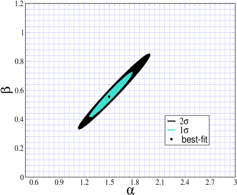
Figure 1: Allowed regions in the parameter space $\alpha-\beta$ at 1$\sigma$ and 2$\sigma$ confidence level from the combined analysis of SNe Ia data and OHD

Using these values of $\alpha$ and $\beta$ as obtained from the analysis we can determine the time dependence of the scale factor and the Hubble parameter.

IV Determining $\phi(t)$ and $F(X)$ from the analysis of SNe Ia data

For a flat universe, which is consistent with the current bounds from WMAP observation on the ratio of the energy density in curvature to the critical density, $|\Omega_{K}^{0}|<0.01$ (95% confidence level)ref:komatsu , the Hubble parameter $H(z)$ corresponding to a redshift $z$ is directly related to the luminosity distance through the relation

$$E(z) \equiv \frac{H(z)}{H_{0}}=\left[\frac{d}{dz}\left(\frac{D_{L}(z)}{1+z}\right)\right]^{-1}$$ (24)

From the equations $H=\displaystyle\frac{\dot{a}}{a}$ and $\displaystyle\frac{a_{0}}{a}=1+z$ we get $dt=-\displaystyle\frac{dz}{(1+z)H}$. Using this relation its useful to introduce a dimensionless parameter $\tau$ as

$$\tau(z) \equiv H_{0}\Big{(}t(z)-t_{0}\Big{)}=-\int_{0}^{z}\frac{dx}{(1+x)E(x)}\ .$$ (25)

The present epoch $(t(z=0)\equiv t_{0})$ corresponds to $\tau(z=0)=0$. In this work we consider the parameter $\tau$ to represent time and obtain the numerical solution for $d\phi/d\tau$ satisfying

$$\frac{d\phi}{d\tau}=a^{3}(\tau)\frac{dE}{d\tau}-a(\tau)K\ ,$$ (26)

as derived earlier in Eq. (9).

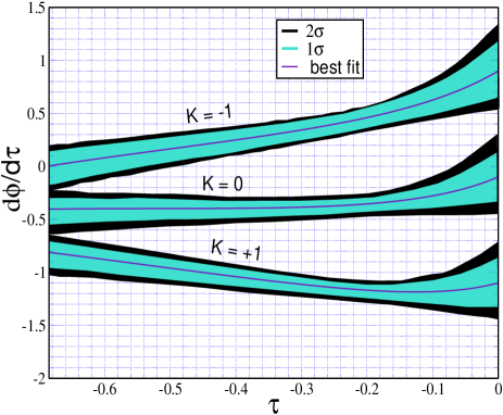
Figure 2: Plot of $d\phi/d\tau$ vs $\tau$ for $K=+1,0,-1$. Solid lines represent the plots drawn for best-fit values of $\alpha$ and $\beta$. The corresponding 1$\sigma$ and 2$\sigma$ variations are shown by shaded regions.

Using Eqs. (15), (24) and (25), with the values of $\alpha$ and $\beta$ as obtained from the analysis, we can numerically obtain the dependence of $E(z)$ and $\tau(z)$ on $z$. From these the time($\tau$)-dependence of $E$ can be extracted. We use this to evaluate $\frac{dE}{d\tau}$ as a function of $\tau$. Similarly from the equations $a=a_{0}/(1+z)$ and (25) the time variation of the scale factor can be obtained. All through the work we have assumed that the scale factor at present epoch is normalized to unity ($a_{0}=1$). Substituting the solutions for $dE/d\tau(\tau)$ and $a(\tau)$ in Eq. (26) we finally compute $d\phi/d\tau$ as a function of time ($\tau$). In Figure. 2 we have shown the variation of $d\phi/d\tau$ with $\tau$ for all the three different values of the curvature constant $K$. The solid curves in this figure represent the estimated variation corresponding to the best-fit values of $\alpha$ and $\beta$ (Eq. (23) ) obtained from the analysis. Using the 1$\sigma$ and 2$\sigma$ ranges of the parameters $\alpha$ and $\beta$ allowed from the analysis, we also obtain the corresponding spreads in the $d\phi/d\tau$-$\tau$ variation. These are shown by the shaded regions in Figure. 2. It is important to note from the results that, for $K=0\ (+1)$, $d\phi/d\tau=0$ is disfavoured above 2$\sigma$ (1$\sigma$) level all of the epochs probed in SNe Ia observations. For $K=-1$, however, a zero value of $d\phi/d\tau$ remains allowed within 2$\sigma$ level only for some earlier epochs of time accessible in SNe Ia observations.

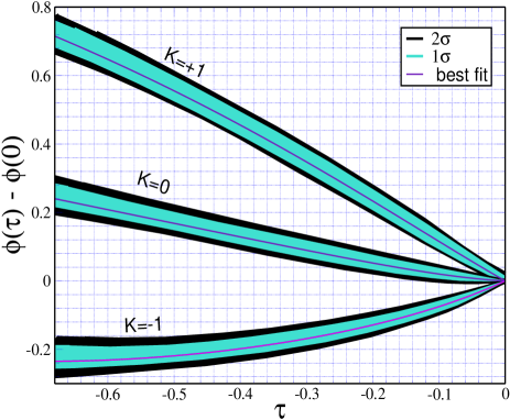
Figure 3: Plot of $\phi(\tau)-\phi(0)$ vs $\tau$ for $K=+1,0,-1$. Solid lines represent the plots drawn for best-fit values of $\alpha$ and $\beta$. The corresponding 1$\sigma$ and 2$\sigma$ variations are shown by shaded regions.

Integrating Eq. (26) and using the values of $\alpha$ and $\beta$ as obtained from the analysis, we find that the obtained time dependence of $\phi(\tau)$ can be fitted with

$$\phi(\tau)-\phi(0) \sim \lambda_{1}\tau+\lambda_{2}\tau^{2}$$ (27)

to an appreciable extent of statistical precision. We present the results in Figure 3 where we have plotted $\phi(\tau)-\phi(0)$ as a function of $\tau$ for three different values of $K$. The solid curves and shaded regions in Figure 3, respectively, represent the plots corresponding to the best-fit values of $(\alpha,\beta)$ and their 1$\sigma$ and 2$\sigma$ uncertainties. The observational data are also instrumental in not providing room for further higher order terms of $\tau$ in the obtained time dependence of $\phi$. To find the values of $\lambda_{1}$ and $\lambda_{2}$ based on observational data and also to have a quantitative estimation of how good a form like Eq. (27) can accommodate the obtained time dependence of $\phi$ from analysis of observational data, we minimize the following $\tilde{\chi}^{2}$ function with respect to the parameters $\lambda_{1}$ and $\lambda_{2}$,

$$\tilde{\chi}^{2} = \sum_{i=1}^{n}\left[\frac{\Phi_{\rm est}(\tau_{i})-\Phi_{\rm fit}(\tau_{i},\lambda_{1},\lambda_{2})}{\Delta\Phi_{\rm est}(\tau_{i})}\right]^{2}$$ (28)

where $\Phi_{\rm est}(\tau_{i})\equiv\phi(\tau_{i})-\phi(0)$ is estimated in a way as described after Eq. (26) and $\Phi_{\rm fit}(\tau_{i},\lambda_{1},\lambda_{2})=\lambda_{1}\tau_{i}+\lambda_{2}{\tau_{i}}^{2}$. $\Delta\Phi_{\rm est}(\tau_{i})$ is the average value of estimated 1$\sigma$ uncertainty in $\Phi_{\rm est}(\tau_{i})$. $n$ is the total number of points $(\tau_{i},\Phi_{\rm est}(\tau_{i}))$ considered (distributed within time range accessible in SNe Ia observations) for this particular analysis. We choose a large $n(=50)$ so that $\tilde{\chi}^{2}_{\rm minimum}/n$ provides measure of $\tilde{\chi}^{2}$ per degree of freedom. The best-fit values of the parameters $\lambda_{1}$ and $\lambda_{2}$ from this analysis for all three different values of curvature constant along with the corresponding values of $\tilde{\chi}^{2}/n$ at the best-fit (minimum $\chi^{2}$) are listed in Table 1. We also find the 1$\sigma$ and 2$\sigma$ allowed ranges for the parameters $\lambda_{1}$ and $\lambda_{2}$ which in this case of 2-parameter fit correspond to $\tilde{\chi}^{2}\leq\tilde{\chi}^{2}_{\rm minimum}+2.30$ and $\tilde{\chi}^{2}\leq\tilde{\chi}^{2}_{\rm minimum}+6.17$, respectively. The ranges are shown by shaded regions in Figure 4, where the best-fit points are also marked. At a quantitative level, very low values of $\tilde{\chi}^{2}_{\rm minimum}/n$ ($\ll 1$) is a phenomenological indication of the fact that the time dependence of the $k$-essence field as extracted from observational data can be very convincingly accommodated within a profile: $\phi_{\rm k-essence}(t)\sim\lambda_{0}+\lambda_{1}\ \tau+\lambda_{2}\ \tau^{2}$. The results of the analysis show that for $K=1(-1)$ both $\lambda_{1}$ and $\lambda_{2}$ are negative (positive) at 2$\sigma$ confidence level. For $K=0$, $\lambda_{1}$($\lambda_{2}$) is negative(positive) at 2$\sigma$ confidence level.

Table 1: Values of $\lambda_{1}$, $\lambda_{2}$ and $\tilde{\chi}^{2}_{\rm minimum}/n$ for $K=1,0,-1$.

$K$	$\lambda_{1}$	$\lambda_{2}$	$\tilde{\chi}^{2}_{\rm minimum}/n$
+1	-1.22	-0.23	0.02
0	-0.23	0.208	0.03
-1	0.76	0.64	0.035

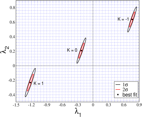
Figure 4: Best-fit values of the parameters $\lambda_{1}$ and $\lambda_{2}$ with their 1$\sigma$ and 2$\sigma$ allowed ranges.

Finally Eq. (10) can be rewritten in terms of the dimensionless time parameter $\tau$. Then using the $\tau$-dependence of the $k$-essence scalar field $\phi$ as obtained above from the analysis of observational data, the $X$-dependence of the quantity $[F(X)-F(X_{0})]/\sqrt{2C}$ can be found by the method as described in Sec. II. The plots are shown in Fig. 5 for three different values of curvature constant $K$. This accommodates a wide spectrum of forms for the function $F(X)$ because of the arbitrariness of the constant $C$ appearing in the scaling relation.

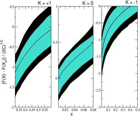
Figure 5: Plot of the quantity $[F(X)-F(X_{0})]/\sqrt{2C}$ vs $X$ with their 1$\sigma$ and 2$\sigma$ allowed ranges as obtained from analysis of observational data

V Discussions and Conclusions

In this work we have shown that a model of $k$-essence incorporating a scaling relation can be accommodated within the luminosity distance - redshift data observed for type Ia Supernova. Existence of the scaling relation within the framework of $k$-essence model allows to establish contact between the spatially homogeneous $k$-essence scalar field, and the scale factor and the Hubble parameter associated with the expansion of the FRW universe. Estimation of the time dependences of the cosmological quantities - the scale factor and the Hubble parameter from the observed SNe Ia data thus allows one to find temporal behaviour of the $k$-essence field $\phi(\tau)$. This comes out to be $\phi(t)\sim\lambda_{0}+\lambda_{1}\tau+\lambda_{2}\tau^{2}$ where $\lambda_{i}$ are constants and have been determined from the analysis of the observational data along with their uncertainties. With the obtained time dependence of the scalar field $\phi$, the use of scaling relation helps to obtain the form of the function $F(X)-F(X_{0})$ up to an arbitrary multiplicative constant occurring in the scaling relation itself. We have also presented the 1$\sigma$ and 2$\sigma$ ranges of this dependence as allowed from the observational data.

Time dependences of the $k$-essence scalar field extracted from SNe Ia observations within its accessible time domain viz $0.9<t/t_{0}<1.0$ are similar to that of a quintessence field responsible for homogeneous inflation which occurs at an epoch $t/t_{0}$ very close to zero. Note that these two domains correspond to $-0.7<\tau<0$ ($k$-essence) and $\tau\to-\infty$ (quintessence), respectively, in our treatment. The temporal domains of the two scalar fields ($k$-essence and quintessence) are well separated. Therefore, similar scalar fields (so far as their time evolution is concerned) can account for inflation as well as dark energy driven accelerated expansion. Our work seems to indicate that this view has some observational support. Also note that the scaling relation implies that for well behaved $F(X)$, $X$ cannot go to zero. This is borne out by the above results.

A more realistic model would have included dust matter. However, this entails $\rho$ in Eqs. (3-6) being replaced by $\rho+\rho_{\rm dust~{}matter}$. Further, a choice would have to be made regarding the form of $\rho_{\rm dust~{}matter}$. Consequently the scaling relation (Eq. 7) is no longer valid. This problem is presently under investigation.

References

- (1) S. Perlmutter et al., Astrophys. J. 517, 565 (1999)
- (2) A. G. Riess et al., Astron. J. 116, 1009 (1998)
- (3) A. G. Riess et al., Astrophys. J. 607, 665 (2004)
- (4) A. G. Riess et al., Astrophys. J. 659, 98 (2007)
- (5) P. Astier et al. Astron. Astrophys. 447, 31 (2006)
- (6) W. M. Wood-Vasey et al., Astrophys. J. 666, 694 (2007)
- (7) M. Hicken et al., Astrophys. J. 700, 1097 (2009)
- (8) M. Kowalski et al. Astrophys. J. 686, 749 (2008)
- (9) D. J. Eisenstein et al. Astrophys. J. 633, 560 (2005)
- (10) S. Cole et al. Mon. Not. Roy. Astron. Soc. 362, 505 (2005)
- (11) G. Huetsi, Astron. Astrophys. 449, 891 (2006)
- (12) W. J. Percival et al., Astrophys. J. 657, 51 (2007)
- (13) G. Hinshaw et al., Astrophys. J. Suppl. 180, 225 (2009)
- (14) E. Komatsu et al. , Astrophys. J. Suppl. 192, 18 (2011)
- (15) S. Weinberg, Rev. Mod. Phys. 61, 1 (1989)
- (16) Y. Fujii, Phys. Rev. D26, 2580 (1982); R. D. Peccei, J. Sola, and C. Wetterich, Phys. Lett. B195, 183 (1987); L. H. Ford, Phys. Rev. D35, 2339 (1987); C. Wetterich, Nucl. Phys. B302, 668 (1988); B. Ratra and P. J. E. Peebles, Phys. Rev. D37, 3406 (1988); Y. Fujii and T. Nishioka, Phys. Rev. D42, 361 (1990); T. Chiba, N. Sugiyama, and T. Nakamura, Mon. Not. Roy. Astron. Soc. 289 (1997); P. G. Ferreira and M. Joyce, Phys. Rev. Lett. 79, 4740 (1997); P. G. Ferreira and M. Joyce, Phys. Rev. D58, 023503 (1998); R. R. Caldwell, R. Dave, and P. J. Steinhardt, Phys. Rev. Lett. 80, 1582 (1998); S. M. Carroll, Phys. Rev. Lett. 81, 3067 (1998); E. J. Copeland, A. R. Liddle, and D. Wands, Phys. Rev. D57, 4686 (1998); I. Zlatev, L. M. Wang, and P. J. Steinhardt, Phys. Rev. Lett. 82, 896 (1999); P. J. Steinhardt, L. M. Wang, and I. Zlatev, Phys. Rev. D59, 123504 (1999); A. Hebecker and C. Wetterich, Phys. Rev. Lett. 85. 3339 (2000); A. Hebecker and C. Wetterich, Phys. Lett. B497, 281 (2001)
- (17) C.Armendariz-Picon, T.Damour and V.Mukhanov, Phys.Lett. B458 209 (1999).
- (18) C.Armendariz-Picon, V.Mukhanov and P.J.Steinhardt, Phys.Rev. D63 103510 (2001).
- (19) C.Armendariz-Picon, V.Mukhanov and P.J.Steinhardt, Phys.Rev.Lett. 85 4438 (2000)
- (20) C.Armendariz-Picon and E.A.Lim, JCAP 0508(2005) 007
- (21) T. Chiba, T. Okabe and M. Yamaguchi, Phys.Rev. D62 023511 (2000)
- (22) N. Arkani-Hamed, H. C. Cheng, M. A. Luty and S. Mukohyama, JHEP 05 (2004) 074, JCAP 0404 (2004) 001
- (23) R.R.Caldwell, Phys.Lett.B545 (2002) 23
- (24) S. Capozziello, Int. J. Mod. Phys. D11, 483 (2002)
- (25) S. Capozziello, V. F. Cardone, S. Carloni, and A. Troisi, Int. J. Mod. Phys. D12, 1969 (2003)
- (26) S. M. Carroll, V. Duvvuri, M. Trodden, and M. S. Turner, Phys. Rev. D70, 043528 (2004)
- (27) L. Amendola, Phys. Rev. D60, 043501 (1999)
- (28) J. P. Uzan,Phys. Rev. D59, 123510 (1999)
- (29) T. Chiba, Phys. RevḊ60, 083508, (1999)
- (30) N. Bartolo and M. Pietroni, Phys. Rev. D61, 023518 (2000)
- (31) F. Perrotta, C. Baccigalupi, and S. Matarrese, Phys. Rev. D61, 023507 (2000)
- (32) G. R. Dvali, G. Gabadadze, and M. Porrati, Phys. Lett. B485, 208 (2000)
- (33) V. Sahni and Y. Shtanov, JCAP 0311, 014 (2003)
- (34) M.Born and L.Infeld, Proc.Roy.Soc.Lond A144(1934) 425.
- (35) P.A.M.Dirac, Royal Society of London Proceedings Series A 268 (1962) 57.
- (36) J.Callan, G.Curtis and J.M.Maldacena, Nucl.Phys. B513 (1998) 198
- (37) G.W.Gibbons, Nucl.Phys. B514 (1998) 603
- (38) G.W.Gibbons, Rev.Mex.Fis. 49S1 (2003) 19
- (39) A.Sen, JHEP 04 (2002) 048
- (40) R.J. Scherrer ,Phys.Rev.Lett. 93 011301 (2004)
- (41) L.P.Chimento, Phys.Rev.D69 123517 (2004) [astro-ph/0311613].
- (42) E. Elizalde, S. Nojiri, S. D. Odintsov, D. Saez-Gomez, Eur.Phys.J.C70,351-361 (2010)[aRxiv:1006.3387]
- (43) S. Nojiri,S. D. Odintsov [arXiv:1008.4275]
- (44) E. Elizalde, S. Nojiri, S. D. Odintsov, L. Sebastian, S. Zerbini, Phys.Rev.D83 086006 (2011); [arXiv:1012.2280]
- (45) J. Simon, L. Verde and R. Jimenez, Phys. Rev. D 71, 123001 (2005)
- (46) V. D. Barger and D. Marfatia, Phys. Lett. B 498, 67 (2001) [arXiv:astro-ph/0009256].
- (47) A. A. Sen, JCAP 0603 , 010 (2006)
- (48) S. Tsujikawa, arXiv:hep-ph/0304257.
- (49) V. Mukhanov, “Physical Foundations of Cosmology”, Cambridge (2005)
- (50) T. Padmanabhan and T. R. Choudhury, Mon. Not. Roy. Astron. Soc. 344, 823 (2003)
- (51) T. M. Davis et al., Astrophys. J. 666, 716 (2007)
- (52) R. Kessler et al., Astrophys. J. Suppl. 185 , 32 (2009)
- (53) R. Amanullah et al., Astrophys. J. 716, 712 (2010)
- (54) L. Xu, Y. Wang, JCAP 1006, 002 (2010)
- (55) R. G. Abraham et al., Astron. J. 127, 2455 (2004)
- (56) E. Gaztanaga, A. Cabre, L. Hui, Mon. Not. Roy. Astron. Soc. 399, 166 (2009)
- (57) A. G. Riess et al., Astrophys. J. 699, 539 (2009)
- (58) D. Stern, R. Jimenez, L. Verde, M. Kamionkauski, S. A. .Stanford, JCAP 1002, 008 (2010)
- (59) D.Gangopadhyay and S. Mukherjee, Phys. Lett.B665 121 (2008)
- (60) D.Gangopadhyay, Gravitation and Cosmology 16 231 (2010)