Effective surface motion on a reactive cylinder of particles that perform intermittent bulk diffusion

Abstract

In many biological and small scale technological applications particles may transiently bind to a cylindrical surface. In between two binding events the particles diffuse in the bulk, thus producing an effective translation on the cylinder surface. We here derive the effective motion on the surface, allowing for additional diffusion on the cylinder surface itself. We find explicit solutions for the number of adsorbed particles at one given instant, the effective surface displacement, as well as the surface propagator. In particular sub- and superdiffusive regimes are found, as well as an effective stalling of diffusion visible as a plateau in the mean squared displacement. We also investigate the corresponding first passage and first return problems.

I Introduction

Bulk mediated surface diffusion (BMSD) defines the effective surface motion of particles, that intermittently adsorb to a surface or diffuse in the contiguous bulk volume. As sketched in Fig. 1 for a cylindrical surface, the particle, say, starts on the surface and diffuses along this surface with diffusion constant $D_{s}$. Eventually the particle unbinds, and performs a three-dimensional stochastic motion in the adjacent bulk, before returning to the surface. Typically, the values of $D_{b}$ are significantly larger than $D_{s}$. The recurrent bulk excursions therefore lead to decorrelations in the effective surface motion of the particle, and thus to a more efficient exploration of the surface.

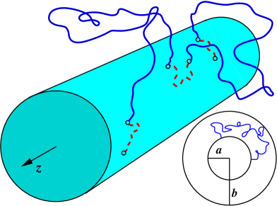
Figure 1: A particle diffuses in the bulk (full lines) and intermittently binds to a cylinder surface on which it may also diffuse (broken lines). This produces an effective surface motion. We here consider the motion along the cylinder. Bottom right: frontal of diffusion between inner and outer cylinder.

Theoretically BMSD was previously investigated for a planar surface in terms of scaling arguments bychuk ; bychuk1 , master equation schemes revelli , and simulations fatkullin . More recently the first passage problem between particle unbinding and rebinding for a free cylindrical surface was derived levitz . Following our short communication rc we here present in detail an exact treatment of BMSD for a reactive cylindrical surface deriving explicit expressions for the surface occupation, the effective mean squared displacement (MSD) along the surface, and the returning time distribution from the bulk. In this approach different dynamic regimes arise naturally from the physical timescales entering our description. Thus at shorter times we derive the famed superdiffusive surface spreading with surface MSD of the form $\langle z^{2}(t)\rangle\sim t^{3/2}$ report ; igor and the associated Cauchy form of the surface probability density function (PDF). At longer times we obtain an a priori unexpected leveling off of the surface MSD, representing a tradeoff between an increasing number of particles that escape into the bulk and the increasing distance on the surface covered in ever-longer bulk excursions for those particles that do return to the surface. Only when the system is confined by an outer cylinder eventually normal surface diffusion will emerge. Apart from the Lévy walk-like superdiffusive regime the rich dynamic behavior found here are characteristic of the cylindrical geometry.

Nuclear magnetic resonance (NMR) measurements of liquids in porous media are sensitive to the preferred orientation of adsorbate molecules on the local pore surface, such that surface diffusion on such a non-planar surface produces spin reorientations and remarkably long correlations times kimmich . Apart from pure surface diffusion the experiment by Stapf et al. clearly showed the influence of BMSD steps and the ensuing Lévy walk-like superdiffusion stapf . More recently NMR techniques were used to unravel the effective surface diffusion on cylindrical mineralic rods levitz , supporting, in particular, the first passage behavior with its typical logarithmic dependence. BMSD on a cylindrical surface is also relevant for the transient binding of chemicals to nanotubes nanotubes and for numerous other technological applications bychuk1 . In a biological context, BMSD along a cylinder is intimately related to the diffusive dynamics underlying gene regulation bvh ; berg : DNA binding proteins diffuse not only in the bulk but intermittently bind non-specifically to the DNA, approximately a cylinder, and perform a one-dimensional motion along the DNA chain, as proved experimentally wang ; bonnet . The interplay between bulk and effective surface motion improves significantly the search process of the protein for its specific binding site on the DNA. Similarly the net motion of motor proteins along cytoskeletal filaments is also affected by bulk mediation. Namely, the motors can fall off the cellular tracks and then rebind to the filament after a bulk excursion motor . Outside of biological cells the exchange behavior between cell surface and surrounding bulk is influenced by bulk excursions, the cylindrical geometry being of relevance for a large class of rod-shaped bacteria (bacilli) and their linear arrangements bacillus .

The dynamics revealed by our approach may also be important for the quantitative understanding of colonialization processes on surfaces in aqueous environments when convection is negligible: suppose that bacteria stemming from a localized source, for instance, near to a submarine hot vent, start to grow on an offshore pipeline. From this mother colony new bacteria will be budding and enter the contiguous water. The Lévy dust-like distribution due to BMSD will then make sure that bacteria can start a new colony, that is disconnected from the former, and therefore give rise to a much more efficient spreading dynamics over the pipeline.

In all these examples it is irrelevant which specific trajectory the particles follow in the bulk, the interesting part is the effective motion on the cylinder surface. We here analyze in detail this bulk mediated surface diffusion on a long cylinder.

II Characteristic time scales and important results

In this Section we introduce the relevant time scales of the problem of bulk mediated surface diffusion of the cylindrical geometry presented in Fig. 1 and collect the most important results characteristic for the effective surface motion of particles. As we are interested only in the motion along the cylinder axis $z$, we consider the rotationally symmetric problem with respect to the polar angle $\theta$, that will therefore not appear explicitly in the following expressions (compare also Sec. III). Since the full analytical treatment of the problem involves tedious calculations we first give an overview of the most important results, leaving the derivations to the forthcoming Sections and Appendices.

II.1 Characteristic time scales

Using the result (48) for the Fourier-Laplace transform $n(k,s)$ of the density of particles on the cylinder surface, we compute the Laplace transform of the number of surface particles,

$$N_{s}(s) = \int_{-\infty}^{\infty}n(z,s)dz=n(k,s)\Big{|}_{k=0}$$ (1)

$$= \frac{N_{0}}{\displaystyle s+\kappa\sqrt{\frac{s}{D_{b}}}\frac{\Delta_{1}(0,s)}{\Delta(0,s)}},$$

where $\kappa$ is a surface-bulk coupling constant defined below, $D_{b}$ is the bulk diffusion constant,

$$\Delta_{1}(0,s) = K_{1}(a\xi)I_{1}(b\xi)-I_{1}(a\xi)K_{1}(b\xi),$$

$$\Delta(0,s) = I_{0}(a\xi)K_{1}(b\xi)+K_{0}(a\xi)I_{1}(b\xi),$$ (2)

and $\xi\equiv\sqrt{s/D_{b}}$. The $I_{\nu}$ and $K_{\nu}$ denote modified Bessel functions. We define the Laplace and Fourier transforms of the surface density $n(z,t)$ through

$$n(k,t)=\mathscr{F}\{n(z,t)\}=\int_{-\infty}^{\infty}e^{ikz}n(z,t)dz$$ (3)

and

$$n(z,s)=\mathscr{L}\{n(z,t)\}=\int_{0}^{\infty}e^{-st}n(z,t)dt.$$ (4)

Here and in the following we express the transform of a function by explicit dependence on the Fourier or Laplace variable, thus, $n(k,s)$ is the Fourier-Laplace transform of $n(z,t)$.

From expression (1) we recognize that in the limit $\kappa\to 0$ the number of particles on the cylinder surface does not change, i.e., $N(t)=N_{0}$. The coupling parameter according to Eq. (49) is connected to the unbinding time scale $\tau_{\mathrm{off}}$, the bulk diffusivity $D_{b}$, and the binding rate $k_{b}$ through $\kappa=D_{b}/[k_{b}\tau_{\mathrm{off}}]$. Vanishing $\kappa$ therefore corresponds to an infinite time scale for unbinding. This observation allows us to introduce a characteristic coupling time

$$t_{\kappa}\equiv\frac{D_{b}}{\kappa^{2}}=\frac{k_{b}^{2}\tau_{\mathrm{off}}^{2}}{D_{b}}.$$ (5)

Note that the binding constant $k_{b}$ has dimension $\mathrm{cm}/\mathrm{sec}$, see Section III. As in the governing equations the coupling constant $\kappa$ and the bulk diffusivity $D_{b}$ are the relevant parameters, the characteristic time $t_{\kappa}$ in a scaling sense is uniquely defined. When the coupling between bulk and cylinder surface is weak, $\kappa\to 0$, the corresponding coupling time $t_{\kappa}$ diverges. It vanishes when the coupling is strong, $\kappa\to\infty$.

While the time scale $t_{\kappa}$ is characteristic of the bulk-surface exchange, the geometry of the problem imposes two additional characteristic times. Namely, the inner and outer cylinder radii involve the time scales

$$t_{a}\equiv\frac{a^{2}}{D_{b}}$$ (6)

and

$$t_{b}\equiv\frac{b^{2}}{D_{b}},$$ (7)

respectively. By definition, $t_{b}$ is always larger than $t_{a}$. For times shorter than the scale $t_{a}$ a diffusing particle behaves as if it were facing a flat surface, while for times longer then $t_{a}$ it can sense the cylindrical shape of the surface. Similarly, $t_{b}$ defines the scale when a particle starts to engage with the outer cylinder and therefore senses the confinement. With the help of these time scales we can rewrite expression (1) for the number of surface particles in the form

$$N_{s}(s)=\frac{N_{0}t_{\kappa}^{1/2}}{s^{1/2}\Big{(}(st_{\kappa})^{1/2}+\Delta_{1}(0,s)/\Delta(0,s)\Big{)}},$$ (8)

where

$$\Delta_{1}(0,s)=K_{1}\left(\sqrt{st_{a}}\right)I_{1}\left(\sqrt{st_{b}}\right)-I_{1}\left(\sqrt{st_{a}}\right)K_{1}\left(\sqrt{st_{b}}\right)$$ (9)

and

$$\Delta(0,s)=I_{0}\left(\sqrt{st_{a}}\right)K_{1}\left(\sqrt{st_{b}}\right)+K_{0}\left(\sqrt{st_{a}}\right)I_{1}\left(\sqrt{st_{b}}\right).$$ (10)

From the characteristic time scales $t_{\kappa}$, $t_{a}$, and $t_{b}$ we can construct the three limits:

(i) Strong coupling limit

$$t_{\kappa}\ll t_{a}\ll t_{b};$$ (11)

here the shortest time scale is the coupling time. This regime is the most interesting as it leads to the transient Lévy walk-like superdiffusive behavior.

(ii) Intermediate coupling limit

$$t_{a}\ll t_{\kappa}\ll t_{b};$$ (12)

here the superdiffusive regime is considerably shorter, however, an interesting transition regime is observed.

(iii) Weak coupling limit

$$t_{a}\ll t_{b}\ll t_{\kappa}.$$ (13)

To limit the scope of this paper we will not consider this latter case in the following. However, we note that for $t\ll t_{b}$ the behavior will be similar to the $t\ll t_{\kappa}$ part of the intermediate coupling limit (ii).

II.2 Important results

We now discuss the results for the most important quantities characteristic of the effective surface motion. The dynamic quantities we consider are the number of particles $N_{s}(t)$, that are adsorbed to the inner cylinder surface at given time $t$; as well as the one-particle mean squared displacement

$$\langle z^{2}(t)\rangle=\frac{1}{N_{0}}\int_{-\infty}^{\infty}z^{2}n(z,t)dz.$$ (14)

This quantity is biased by the fact that an increasing amount of particles is leaving the surface. To balance for this loss and quantify the effective surface motion for those particles that actually move on the surface, we also consider the ‘normalized’ mean squared displacement

$$\langle z^{2}(t)\rangle_{\mathrm{norm}}=\frac{1}{N_{s}(t)}\int_{-\infty}^{\infty}z^{2}n(z,t)dz.$$ (15)

The detailed behavior of these quantities will be derived in what follows, and we will also calculate the effective surface concentration $n(z,t)$ itself. Here we summarize the results for the surface particle number and the surface mean squared displacements.

II.2.1 Strong coupling limit

In Table 1 we summarize the behavior in the four relevant time regimes for the case of strong coupling. The evolution of the number of particles on the surface turns from an initially constant behavior to an inverse square root decay when the particles engage into surface-bulk exchange. At longer times, the escape of particles to the bulk becomes faster and follows a $1/t$ law. Eventually the confinement by the outer cylinder comes into play, and we reach a stationary limit.

Time regime	$N_{s}(t)$	$\langle z^{2}(t)\rangle$	$\langle z^{2}(t)\rangle_{\mathrm{norm}}$
$t\ll t_{\kappa}$	$N_{0}$	$\displaystyle 2D_{s}t+\frac{4}{3\sqrt{\pi t_{\kappa}}}D_{b}t^{3/2}$	$\displaystyle 2D_{s}t+\frac{4}{3\sqrt{\pi t_{\kappa}}}D_{b}t^{3/2}$
$t_{\kappa}\ll t\ll t_{a}$	$\displaystyle\sqrt{\frac{t_{\kappa}}{\pi}}\frac{N_{0}}{t^{1/2}}$	$\displaystyle 2D_{s}t_{\kappa}+\frac{2\sqrt{t_{\kappa}}}{\sqrt{\pi}}D_{b}t^{1/2}$	$\displaystyle 2\sqrt{\pi t_{\kappa}}D_{s}t^{1/2}+2D_{b}t$
$t_{a}\ll t\ll t_{b}$	$\displaystyle\frac{1}{2}\sqrt{t_{a}t_{\kappa}}\frac{N_{0}}{t}$	$\displaystyle t_{a}t_{\kappa}D_{s}\frac{1}{t}\ln\left(\frac{4t}{Ct_{a}}\right)+\sqrt{t_{a}t_{\kappa}}D_{b}$	$\displaystyle 2\sqrt{t_{a}t_{\kappa}}D_{s}\ln\left(\frac{4t}{Ct_{a}}\right)+2D_{b}t$
$t_{b}\ll t$	$\displaystyle 2\frac{\sqrt{t_{a}t_{\kappa}}}{t_{b}}N_{0}$	$\displaystyle\frac{8t_{a}t_{\kappa}}{t_{b}^{2}}D_{s}t+\frac{4\sqrt{t_{a}t_{\kappa}}}{t_{b}}D_{b}t$	$\displaystyle 4\frac{\sqrt{t_{a}t_{\kappa}}}{t_{b}}D_{s}t+2D_{b}t$

Table 1: Effective surface diffusion, strong coupling limit. For the different regimes we list the number of particles $N_{s}(t)$ on the surface, the surface mean squared displacement $\langle z^{2}(t)\rangle$, and the normalized mean squared displacement $\langle z^{2}(t)\rangle_{\mathrm{norm}}$. $C=\exp(\gamma)\approx 1.78107$ where $\gamma$ is Euler’s constant.

The mean squared displacement has a very interesting initial anomalously diffusive behavior $\simeq t^{3/2}$ report ; igor . This superdiffusion arises due to mediation by bulk excursions resulting in the effective Cauchy distribution

$$n(z,t)\sim\frac{N_{0}\kappa t}{\pi\left(z^{2}+\kappa^{2}t^{2}\right)}.$$ (16)

In this initial regime we can use a simple scaling argument to explain this superdiffusive behavior, compare the discussion in Ref. bychuk . Thus, once detached from the surface a particle returns to the surface with a probability distributed according to $\simeq t^{-1/2}$. Due to the diffusive coupling $z^{2}\simeq t$ in the bulk the effective displacement along the cylinder is then distributed according to $\simeq|z|^{-1}$, giving rise to a probability density $\simeq z^{-2}$.

Later, the mean squared displacement turns over to a square root behavior corresponding to subdiffusion. As can be seen from the associated normalized mean squared displacement, this behavior is due to the escaping particles. At even longer times the mean squared displacement reaches a plateau value. This is a remarkable property of this cylindrical geometry, reflecting a delicate balance between decreasing particle number and increasing length of the bulk mediated surface translocations. This plateau is the terminal behavior when no outer cylinder is present. That is, even at infinite times, when fewer and fewer particles are on the surface, the surface mean squared displacement does not change. In presence of the outer cylinder the mean squared displacement eventually is dominated by the bulk motion and acquires the normal linear growth with time.

Combining the dynamics of the number of surface particles and the mean squared displacement we obtain the behavior of the normalized mean squared displacement listed in the last column.

II.2.2 Intermediate coupling limit

In the intermediate coupling limit the results are listed in Table 2. Also in this regime we observe the initial superdiffusion and associated Cauchy form of the surface particle concentration. The subsequent regime of intermediate times splits up into two subregimes. This subtle turnover will be discussed in detail below. The last two regimes exhibit the same behavior as the corresponding regimes in the strong coupling limit.

Time regime	$N_{s}(t)$	$\langle z^{2}(t)\rangle$	$\langle z^{2}(t)\rangle_{\mathrm{norm}}$
$t\ll t_{a}$	$N_{0}$	$\displaystyle 2D_{s}t+\frac{4}{3\sqrt{\pi t_{\kappa}}}D_{b}t^{3/2}$	$\displaystyle 2D_{s}t+\frac{4}{3\sqrt{\pi t_{\kappa}}}D_{b}t^{3/2}$
$t_{a}\ll t<t_{c}\ll t_{\kappa}$	$N_{0}$	$\displaystyle 2D_{s}t+\frac{2D_{b}t^{2}}{t_{c}\ln^{2}\left(4t/[C^{2}t_{a}]\right)}$	$\displaystyle 2D_{s}t+\frac{2D_{b}t^{2}}{t_{c}\ln^{2}\left(4t/[C^{2}t_{a}]\right)}$
$t_{a}\ll t_{c}<t\ll t_{\kappa}$	transition to $\simeq 1/t$	transition to $\simeq\mathrm{const}$	transition to $\simeq t$
$t_{\kappa}\ll t\ll t_{b}$	$\displaystyle\frac{1}{2}\sqrt{t_{a}t_{\kappa}}\frac{N_{0}}{t}$	$\displaystyle t_{a}t_{\kappa}D_{s}\frac{1}{t}\ln\left(\frac{4t}{Ct_{a}}\right)+\sqrt{t_{a}t_{\kappa}}D_{b}$	$\displaystyle 2\sqrt{t_{a}t_{\kappa}}D_{s}\ln\left(\frac{4t}{Ct_{a}}\right)+2D_{b}t$
$t_{b}\ll t$	$\displaystyle\frac{2\sqrt{t_{a}t_{\kappa}}}{t_{b}}N_{0}$	$\displaystyle\frac{8t_{a}t_{\kappa}}{t_{b}^{2}}D_{s}t+4\frac{\sqrt{t_{a}t_{\kappa}}}{t_{b}}D_{b}t$	$\displaystyle 4\frac{\sqrt{t_{a}t_{\kappa}}}{t_{b}}D_{s}t+2D_{b}t$

Table 2: Effective surface diffusion, intermediate coupling limit.

II.3 Numerical evaluation

In Figs. 2 and 3 we show results from numerical Laplace inversion of the exact expressions for the number of surface particles and the surface mean squared displacement. We consider both the strong and intermediate coupling cases. The parameters fixing the time scales were chosen far apart from each other to distinguish the different limiting behaviors computed in the following Sections. In all figures a vanishing surface diffusivity ($D_{s}=0$) is chosen for clarity.

For strong coupling the selected time scales are $t_{\kappa}=10^{-6}$, $t_{a}=1$, and $t_{b}=10^{6}$ in dimensionless units. Therefore the bulk diffusion constant becomes $D_{b}=a^{2}/t_{a}=25$ for our choice $a=5$. The coupling constant is $\kappa=a/\sqrt{t_{a}t_{\kappa}}=5\times 10^{3}$, and the outer cylinder radius becomes $b=a/\sqrt{t_{b}/t_{a}}=5\times 10^{3}$.

In the intermediate regime we chose $t_{a}=10^{-6}$, $t_{\kappa}=1$, and $t_{b}=10^{6}$. This sets the bulk diffusivity to $D_{b}=25\times 10^{6}$ and the outer cylinder radius to $b=5\times 10^{6}$. These values are chosen such that we can plot the results for the intermediate case alongside the strong coupling case.

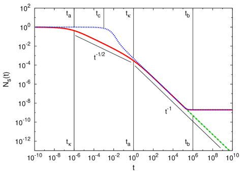
Figure 2: Time evolution of the number of surface particles obtained by numerical Laplace inversion, for the following cases: strong binding with (green dashed-dotted line) and without (red full line) outer cylinder, and intermediate binding in presence of the outer cylinder (blue dashed line). The indicated characteristic time scales correspond to the cases of strong (bottom) and intermediate (top) coupling.

Fig. 2 shows the time evolution of the number of surface particles, normalized to $N_{0}=1$. For the strong coupling case the value remains almost constant until $t\approx t_{\kappa}$, and then turns over to an inverse square root decay that lasts until $t\approx t_{a}$. Subsequently a $t^{-1}$ behavior emerges. In presence of an outer cylinder, due to the confinement this inversely time proportional evolution is finally terminated by a stationary plateau. In the intermediate coupling case similar behavior is observed, apart from the two subregimes in the range at intermediate times.

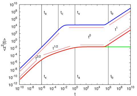
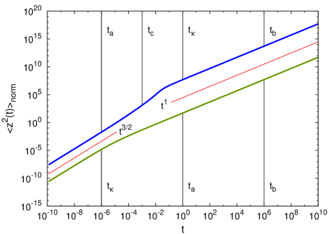
Figure 3: Surface mean squared displacement obtained by numerical Laplace inversion. Left: The graphs show the various effective diffusion regimes $\langle z^{2}(t)\rangle$ along the cylinder. Note the characteristic transient plateau, which is the terminal behavior in the absence of a confining outer cylinder. Right: Normalized function $\langle z^{2}(t)\rangle_{\mathrm{norm}}$. The subregime $t_{c}<t<t_{a}$ in the intermediate case distinctly shows a superdiffusive behavior that is even steeper than the initial $t^{3/2}$ scaling. We show the strong binding case with (red line) and without (green line) and outer cylinder, as well as the case of intermediate binding with outer cylinder (blue line). The characteristic time scales connected with the associated curves denote the cases of strong (bottom) and intermediate (top) coupling.

Fig. 3 depicts the behavior of the surface mean squared displacement. In the left panel the function $\langle z^{2}(t)\rangle$ shows the various regimes found in the strong and intermediate coupling limits. Remarkably the intermediate coupling regime exhibits a superdiffusive behavior in the range $t_{c}<t<t_{a}$ that is even faster than the initial $t^{3/2}$ scaling. The right panel of Fig. 3 shows the behavior of the normalized surface mean squared displacement. See Sections IV and V for details.

III Coupled diffusion equations and general solution

In this Section we state the polar symmetry of the problem we want to consider, and then formulate the starting equations for our model. The general solution is presented in Fourier-Laplace space. In the two subsequent Sections we calculate explicit results in various limiting cases, for strong and intermediate coupling.

III.1 Starting equation and particle number conservation

The full problem is spanned by the coordinates $z$ measured along the cylinder axis, the radius $r$ measured perpendicular to the $z$ axis, and the corresponding polar angle $\theta$. We are only interested in the effective displacement of particles along the cylinder axis and therefore eliminate the $\theta$ dependence. This can be consistently done in the following way. (i) As initial condition we assume that initially the particles are concentrated as a sharp $\delta(z)$ peak on the inner cylinder surface, homogeneous in the angle coordinate $\theta$. (ii) Our boundary conditions are $\theta$ independent.

For the bulk concentration of particles in the volume between the inner and outer cylinders this symmetry requirement simply means that we can integrate out the $\theta$ dependence and consider this concentration as function of $z$, radius $r$, and time $t$: $\mathcal{C}=\mathcal{C}(r,z,t)$. The physical dimension of the concentration $\mathcal{C}$ is $[\mathcal{C}]=1/\mathrm{cm}^{3}$. On the surface of the inner cylinder we measure the concentration by the density $n_{\mathrm{2D}}(z,t)$, which is of dimension $[n_{\mathrm{2D}}]=1/\mathrm{cm}^{2}$. Note that $n_{\mathrm{2D}}(z,t)$ does not explicitly depend on $\theta$. We average this cylinder surface density over the polar angle, and obtain the line density $n(z,t)$:

$$n(z,t)=a\int_{0}^{2\pi}n_{\mathrm{2D}}(z,t)d\theta=2\pi an_{\mathrm{2D}}(z,t),$$ (17)

such that $[n]=1/\mathrm{cm}$. Note that on the inner cylinder with radius $a$ the expression $ad\theta dz$ is the cylindrical surface increment. The factor $2\pi a$ is important when we formulate the reactive boundary condition on the inner cylinder connecting surface line density $n(z,t)$ and the volume density $\mathcal{C}(r,z,t)$.

Given the line density $n$, the total number $N_{s}(t)$ of particles on the inner cylinder surface at given time $t$ becomes

$$N_{s}(t)=\int_{0}^{2\pi}ad\theta\int_{-\infty}^{\infty}n_{\mathrm{2D}}(z,t)dz=\int_{-\infty}^{\infty}n(z,t)dz.$$ (18)

We assume that initially $N_{0}$ particles are concentrated in a $\delta$-peak on the cylinder surface at $z=0$:

$$n(z,t)\Big{|}_{t=0}=N_{0}\delta(z).$$ (19)

Consequently the initial bulk concentration vanishes everywhere on the interval $a<r\leq b$ such that

$$\mathcal{C}(r,z,t)\Big{|}_{t=0}=0.$$ (20)

Let us now specify the boundary conditions at the two cylinder surfaces. At the outer cylinder ($r=b$) we impose a reflecting boundary condition of the Neumann form

$$\frac{\partial}{\partial r}\mathcal{C}(r,z,t)\Big{|}_{r=b}=0.$$ (21)

In the case when we do not consider an outer cylinder ($b\to\infty$) this Neumann condition may be replaced by a natural boundary condition of the form

$$\lim_{r\to\infty}\mathcal{C}(r,z,t)=0.$$ (22)

The reactive boundary condition on the inner cylinder ($r=a$) is derived from a discrete random walk process in App. A (compare also Refs. subsurf ). Accordingly we balance the flux away from the inner cylinder surface,

$$j_{\mathrm{off}}=\frac{1}{\tau_{\mathrm{off}}}n_{\mathrm{2D}}(z,t)=\frac{1}{2\pi a\tau_{\mathrm{off}}}n(z,t),$$ (23)

by the incoming flux from the bulk onto the cylinder surface,

$$j_{\mathrm{on}}=\lim_{r\to a}k_{b}\mathcal{C}(r,z,t).$$ (24)

Here, $\tau_{\mathrm{off}}$ with dimension $[\tau_{\mathrm{off}}]=1/\mathrm{sec}$ is the characteristic time scale for particle unbinding from the surface. It is proportional to the Arrhenius factor of the binding free energy $\varepsilon$ of the particles, $\exp(-|\varepsilon|/[k_{B}T])$, where $k_{B}T$ denotes the thermal energy at temperature $T$. The binding rate $k_{b}$, in contrast, has physical dimension $[k_{b}]=\mathrm{cm}/\mathrm{sec}$, which is typical for surface-bulk coupling in cylindrical coordinates, compare the discussions in Refs. bvh ; berg ; subsurf . For convenience, we collect the coefficients in the reactive boundary condition (24) into the coupling constant

$$\mu\equiv\frac{1}{2\pi ak_{b}\tau_{\mathrm{off}}},$$ (25)

such that our reactive boundary condition finally is recast into the form

$$\mathcal{C}(r,z,t)\Big{|}_{r=a}=\mu n(z,t).$$ (26)

The time evolution of the bulk density $\mathcal{C}(r,z,t)$ is governed by the cylindrical diffusion equation

$$\frac{\partial}{\partial t}\mathcal{C}(r,z,t)=D_{b}\left(\frac{1}{r}\frac{\partial}{\partial r}\left[r\frac{\partial}{\partial r}\right]+\frac{\partial^{2}}{\partial z^{2}}\right)\mathcal{C}(r,z,t),$$ (27)

valid on the domain $a<r<b$ and $-\infty<z<\infty$. In Eq. (27), $D_{b}$ is the bulk diffusion coefficient of dimension $[D_{b}]=\mathrm{cm^{2}}/\mathrm{sec}$. From a random walk perspective we can write $D_{b}=\langle\delta\xi^{2}\rangle/(6\langle\delta\tau\rangle)$, where $\langle\delta\xi^{2}\rangle$ is the average variance of individual jumps, and $\langle\delta\tau\rangle$ is the typical time between consecutive jumps. As shown in App. A the dynamic equation for the line density $n$ directly includes the incoming flux term and is given by

$$\frac{\partial}{\partial t}n=D_{s}\frac{\partial^{2}}{\partial z^{2}}n(z,t)+2\pi aD_{b}\frac{\partial}{\partial r}\mathcal{C}(r,z,t)\Big{|}_{r=a},$$ (28)

where $D_{s}$ denotes the surface diffusion coefficient. In many realistic cases the magnitude of $D_{s}$ is considerably smaller than the bulk diffusivity $D_{b}$. The coupling term connects the surface density $n$ to the bulk concentration $\mathcal{C}$. The fact that here the bulk diffusivity occurs as coupling term stems from the continuum limit, in which the binding rate diverges, and therefore the binding corresponds to the step from the exchange site to the surface.

The diffusion equations (27) and (28) together with the boundary conditions (21) and (26) as well as the initial conditions (19) and (20) completely specify our problem. Moreover the total number of particles is conserved. Namely, the number of surface particles varies with time as

$$\frac{dN_{s}(t)}{dt}=2\pi aD_{b}\int_{-\infty}^{\infty}\frac{\partial}{\partial r}\mathcal{C}(r,z,t)\Big{|}_{r=a}dz,$$ (29)

as can be seen from integration of Eq. (28) over $z$ and noting that $n(|z|\to\infty,t)=0$. For the number of bulk particles we obtain

$$\frac{dN_{b}(t)}{dt} = 2\pi D_{b}\int_{a}^{b}rdr\int_{-\infty}^{\infty}dz\,\frac{1}{r}\frac{\partial}{\partial r}\left(r\frac{\partial}{\partial r}\mathcal{C}(r,z,t)\right)=2\pi D_{b}\int_{-\infty}^{\infty}\left[\left(r\frac{\partial}{\partial r}\mathcal{C}(r,z,t)\right)_{r=b}-\left(r\frac{\partial}{\partial r}\mathcal{C}(r,z,t)\right)_{r=a}\right]$$ (30)

$$= -2\pi aD_{b}\int_{-\infty}^{\infty}\frac{\partial}{\partial r}\mathcal{C}(r,z,t)\Big{|}_{r=a}dz.$$

From these two relations we see that indeed the total number of particles fulfills

$$\frac{d}{dt}\Big{(}N_{s}(t)+N_{b}(t)\Big{)}=0,$$ (31)

and therefore $N_{s}(t)+N_{b}(t)=N_{0}$.

III.2 Solution of the bulk diffusion equation

To solve Eq. (27) and the corresponding boundary and initial value problem we use the Fourier-Laplace transform method. The dynamic equation for $\mathcal{C}(r,k,s)$ is the ordinary differential equation

$$\frac{d^{2}}{dr^{2}}\mathcal{C}(r,k,s)+\frac{1}{r}\frac{d}{dr}\mathcal{C}(r,k,s)-q^{2}\mathcal{C}(r,k,s)=0,$$ (32)

where we use the abbreviation

$$q^{2}=k^{2}+\frac{s}{D_{b}}.$$ (33)

The reactive boundary condition becomes

$$\mathcal{C}(r,k,s)\Big{|}_{r=a}=\mu n(k,s),$$ (34)

and for the reflective condition we find

$$\frac{d}{dr}\mathcal{C}(r,k,s)\Big{|}_{r=b}=0.$$ (35)

The general solution of Eq. (32) is given in terms of the zeroth order modified Bessel functions $I_{0}$ and $K_{0}$ in the linear combination

$$\mathcal{C}(r,k,s)=AI_{0}(qr)+BK_{0}(qr).$$ (36)

The constants $A$ and $B$ follow from the boundary conditions, such that

$$AI_{0}(qa)+BK_{0}(qa)=\mu n(k,s)$$ (37)

and

$$A\frac{\partial}{\partial r}I_{0}(qr)\Big{|}_{r=b}+B\frac{\partial}{\partial r}K_{0}(qr)\Big{|}_{r=b}=0.$$ (38)

Using $\partial I_{0}(qr)/\partial r=qI_{1}(qr)$ and $\partial K_{0}(qr)/\partial r=-qK_{1}(qr)$, we can rewrite the latter relation:

$$AqI_{1}(qb)-BqK_{1}(qb)=0.$$ (39)

The two coefficients are therefore given by

$$A=\frac{K_{1}(qb)}{\Delta(k,s)}\mu n(k,s),\quad B=\frac{I_{q}(qb)}{\Delta(k,s)}\mu n(k,s),$$ (40)

where we introduce the abbreviation

$$\Delta(k,s)\equiv I_{0}(qa)K_{1}(qb)+I_{1}(qb)K_{0}(qa).$$ (41)

Note that, due to the definition of the variable $q$ the function $\Delta$ indeed explicitly depends on the Laplace variable $s$. The solution for the bulk density $\mathcal{C}$ in Fourier-Laplace domain is therefore given by the expression

$$\mathcal{C}(r,k,s)=\frac{\mu n(k,s)}{\Delta(k,s)}\Big{(}K_{1}(qb)I_{0}(qr)+I_{1}(qb)K_{0}(qr)\Big{)}.$$ (42)

III.3 Solution of the surface diffusion equation

In a similar fashion we obtain the Fourier-Laplace transform of the dynamic equation for the surface density $n$, namely

$$sn(k,s)-N_{0}=-k^{2}D_{s}n(k,s)+2\pi aD_{b}\frac{\partial}{\partial r}\mathcal{C}(r,k,s)\Big{|}_{r=a}.$$ (43)

Defining the propagator of the homogeneous equation,

$$G_{s}(k,s)=\frac{1}{s+k^{2}D_{s}},$$ (44)

we find

$$n(k,s)=N_{0}G_{s}(k,s)+G_{s}(k,s)2\pi aD_{b}\frac{\partial}{\partial r}\mathcal{C}(r,k,s)\Big{|}_{r=a}.$$ (45)

From Eq. (42) we obtain for the reactive boundary condition that

$$\frac{\partial}{\partial r}\mathcal{C}(r,k,s)\Big{|}_{r=a}=-\mu n(k,s)\frac{q\Delta_{1}(k,s)}{\Delta(k,s)},$$ (46)

where

$$\Delta_{1}(k,s)\equiv K_{1}(qa)I_{1}(qb)-I_{1}(qa)K_{1}(qb).$$ (47)

Insertion of relation (46) into Eq. (45) produces the result

$$n(k,s)=\frac{N_{0}}{\displaystyle s+k^{2}D_{s}+\kappa q\frac{\Delta_{1}(k,s)}{\Delta(k,s)}}.$$ (48)

Here we also define the coupling constant

$$\kappa\equiv 2\pi a\mu D_{b}=\frac{D_{b}}{k_{b}\tau_{\mathrm{off}}},$$ (49)

which allows us to distinguish the regimes of strong, intermediate, and weak bulk-surface coupling used in this work. If we remove the outer cylinder, that enforces a finite cross-section in the cylindrical symmetry, we obtain the following simplified expression,

$$n(k,s)=\frac{N_{0}}{\displaystyle s+k^{2}D_{s}+\kappa q\frac{K_{1}(qa)}{K_{0}(qa)}},$$ (50)

as in the limit $b\to\infty$, we have $I_{\nu}(qb)\to\infty$ and $K_{\nu}(qb)\to 0$. From the Fourier-Laplace transform (48) the number of particles on the cylinder surface is given by

$$N_{s}(s)=n(k=0,s),$$ (51)

following the definition of the Fourier transform.

Plugging the result (48) into Eq. (42) we obtain the closed form for the Fourier-Laplace transform of the bulk concentration,

$$\mathcal{C}(r,k,s) = \frac{\mu N_{0}}{\Delta(k,s)\Big{(}s+k^{2}D_{s}+\kappa q\Delta_{1}(k,s)/\Delta(k,s)\Big{)}}\Big{(}K_{1}(qb)I_{0}(qr)+I_{1}(qb)K_{0}(qr)\Big{)}$$ (52)

$$= \frac{N_{0}}{2\pi ak_{b}\tau_{\mathrm{off}}}\frac{K_{1}(qb)I_{0}(qr)+I_{1}(qb)K_{0}(qr)}{\Delta(k,s)\Big{(}s+k^{2}D_{s}+\kappa q\Delta_{1}(k,s)/\Delta(k,s)\Big{)}}.$$

We note that the solutions for $n(k,s)$ and $\mathcal{C}(k,s)$ indeed fulfill the particle conservation,

$$\int_{-\infty}^{\infty}n(z,t)dz+2\pi\int_{-\infty}^{\infty}dz\int_{a}^{b}rdr\,\mathcal{C}(r,z,t)=N_{0}\,\,\,\Leftrightarrow\,\,\,n(k,s)\Big{|}_{k=0}+2\pi\int_{a}^{b}rdr\,\mathcal{C}(r,k,s)\Big{|}_{k=0}=\frac{N_{0}}{s}.$$ (53)

Using the results for the surface propagator $n(z,t)$, Eq. (48), we characterize the effective surface diffusion on the cylinder in terms of the single-particle mean squared displacement

$$\langle z^{2}(t)\rangle=N_{0}^{-1}\int_{-\infty}^{\infty}z^{2}n(z,t)dz.$$ (54)

In Fourier-Laplace domain, we re-express this integral as

$$\langle z^{2}(s)\rangle=-N_{0}^{-1}\left.\frac{\partial^{2}n(k,s)}{\partial k^{2}}\right|_{k=0}.$$ (55)

This mean squared displacement includes the unbinding dynamics of particles as manifest in the quantity $N_{s}(t)$. We can exclude this effect by defining the normalized mean squared displacement

$$\langle z^{2}(t)\rangle_{\mathrm{norm}}=\frac{N_{0}}{N_{s}(t)}\langle z^{2}(t)\rangle.$$ (56)

From above results for the effective surface propagator we obtain the exact result for the surface mean squared displacement in App. B. In what follows, however, for simplicity of the argument we proceed differently. Namely we first approximate the effective surface propagator $n(z,t)$, and from the various limiting forms determine the surface mean squared displacement. Comparison to the limits taken from the general results derived in App. B, it can be shown that both procedures yield identical results.

IV Explicit calculations: strong coupling limit

In this Section we consider the strong coupling limit $t_{\kappa}\ll t_{a}\ll t_{b}$, representing the richest of the three regimes. Based on the result for the effective surface propagator, Eq. (48), in Fourier-Laplace space obtained in the previous Section we now calculate the quantities characteristic of the effective motion on the cylinder surface, as mediated by transient bulk excursions. We consider the number of particles on the surface, the axial mean squared displacement, as well as the surface propagator. We divide the discussion into the four different dynamic regimes defined by comparison of the involved time scales $t_{\kappa}$, $t_{a}$, and $t_{b}$.

IV.1 Short times, $t\ll t_{\kappa}\ll t_{a}\ll t_{b}$

The short time limit $t\ll t_{\kappa}\ll t_{a}\ll t_{b}$ corresponds to the Laplace domain regime

$$st_{\kappa},st_{a},st_{b}\gg 1.$$ (57)

IV.1.1 Surface propagator in Fourier-Laplace space

We first obtain the short time limit of the effective surface propagator in Fourier-Laplace space. To this end we note that the following inequalities hold:

$$qa=a\sqrt{k^{2}+\frac{s}{D_{b}}}\geq a\sqrt{\frac{s}{D_{b}}}=\sqrt{st_{a}}\gg 1,$$ (58)

and thus we have

$$qa\gg 1\,\,\,\mbox{and}\,\,\,qb\gg 1.$$ (59)

For this case we use the following expansion of the Bessel functions contained in the abbreviations $\Delta(k,s)$ and $\Delta_{1}(k,s)$. Namely, for $z\to\infty$,

$$I_{\nu}(z)\sim\frac{\exp(z)}{\sqrt{2\pi z}},\,\,\,K_{\nu}(z)\sim\sqrt{\frac{\pi}{2z}}\exp(-z).$$ (60)

From expressions (41) and (47) we find

$$\Delta(k,s)\sim\Delta_{1}(k,s)\sim\frac{\exp(q[b-a])}{2q\sqrt{ab}}.$$ (61)

Therefore, the surface propagator in Fourier-Laplace in the short time limit reduces to the simplified form

$$n(k,s)\sim\frac{N_{0}}{s+k^{2}D_{s}+\kappa\sqrt{k^{2}+s/D_{b}}}.$$ (62)

IV.1.2 Number of particles on the surface

From the relation $N_{s}(s)=n(k=0,s)$ we obtain the number of surface particles by help of the above expression for the limiting form of $n(k,s)$:

$$N_{s}(s)\sim\frac{N_{0}t_{\kappa}}{st_{\kappa}+\sqrt{st_{\kappa}}}.$$ (63)

Since $st_{\kappa}\gg 1$ the leading behavior follows

$$N_{s}(s)\sim\frac{N_{0}}{s},$$ (64)

i.e., we recover that the number of particles on the surface remains approximately conserved in the short time regime,

$$N_{s}(t)\sim N_{0}.$$ (65)

IV.1.3 Surface mean squared displacement

The surface mean squared displacement is readily obtained from the limiting form of the surface propagator (62) by help of relation (55). Namely, we obtain

$$\langle z^{2}(s)\rangle\sim\frac{2D_{s}+D_{b}/\sqrt{st_{\kappa}}}{\left(s+s/\sqrt{st_{\kappa}}\right)^{2}}.$$ (66)

Since $st_{\kappa}\gg 1$ the leading behavior corresponds to

$$\langle z^{2}(s)\rangle\sim\frac{2D_{s}}{s^{2}}+\frac{D_{b}}{t_{\kappa}^{1/2}s^{5/2}},$$ (67)

from which the time-dependence

$$\langle z^{2}(t)\rangle\sim\langle z^{2}(t)\rangle_{\mathrm{norm}}\sim 2D_{s}t\left[1+\frac{2}{3\pi^{1/2}}\frac{D_{b}}{D_{s}}\left(\frac{t}{t_{\kappa}}\right)^{1/2}\right].$$ (68)

yields after Laplace inversion. As in this short time regime $N_{s}(t)\sim N_{0}$, the normalized surface mean squared displacement follows the same behavior.

Remarkably, result (68) contains a contribution growing like $\simeq t^{3/2}$. This superdiffusive behavior becomes relevant when $D_{b}\gg D_{s}$, which is typically observed in many systems. Thus for DNA binding proteins the bulk diffusivity may be a factor of $10^{2}$ or more larger than the diffusion constant along the DNA: for Lac repressor the bulk diffusivity is of the order of $5..9\times 10^{-7}\mathrm{cm}^{2}/\mathrm{sec}$, while the one-dimensional diffusion constant along the DNA surface ranges in between $2..9\times 10^{-10}\mathrm{cm}^{2}/\mathrm{sec}$ wang ; winter .

IV.1.4 Surface propagator in real space

We now turn to the functional form of the surface propagator $n(z,t)$ in real space at short times in the strong coupling limit. We investigate this quantity in the limit $D_{s}=0$ of vanishing surface diffusion.

In the current short time limit $t\ll t_{\kappa}\ll t_{a}\ll t_{b}$ we distinguish two parts of the surface density $n$. Let us start with the central part defined by $k^{2}\gg s/D_{b}$. The corresponding limiting form of Eq. (62) is then given by

$$n(k,s)\sim\frac{N_{0}}{s+\kappa|k|}.$$ (69)

The inverse Fourier-Laplace transform leads to the Cauchy probability density function

$$n(z,t)\sim\frac{N_{0}\kappa t}{\pi\left(z^{2}+\kappa^{2}t^{2}\right)}.$$ (70)

This central part of the surface propagator obeys the governing dynamic equation report ; chechkin_jsp

$$\frac{\partial}{\partial\kappa t}n(z,t)=\frac{\partial}{\partial|z|}n(z,t)$$ (71)

with initial condition $n(z,t=0)=N_{0}\delta(z)$. Here, we defined the space fractional derivative $\partial/\partial|z|$ in the Riesz-Weyl sense whose Fourier transform takes on the simple form samko

$$\int_{-\infty}^{\infty}e^{ikz}\left(\frac{\partial}{\partial|z|}n(z,t)\right)dz=-|k|n(k,t).$$ (72)

Eq. (70) and the corresponding dynamic equation (71) are remarkable results, which are analogous to the findings in Ref. bychuk1 for a flat surface obtained from scaling arguments REMM . It says that the bulk mediation causes an effective surface motion whose propagator is a Lévy stable law of index 1. This behavior can be guessed from the scaling of the returning probability to the surface, together with the diffusive scaling $z^{2}\simeq t$. However, the resulting Cauchy distribution cannot have an infinite range, as the particle in a finite time only diffuses a finite distance. The question therefore arises whether there exists a cutoff of the Cauchy law, and of what form this is.

The advantage of our exact treatment is that the Cauchy law can be derived explicitly, but especially the transition to other regimes studied. To this end we introduce the time-dependent length scale

$$\ell_{C}(t)=\sqrt{D_{b}t}$$ (73)

which turns out to define the range of validity of the Cauchy region. Namely, while at distances $z>\ell_{C}(t)$ we observe a cutoff of the Cauchy behavior, for $z<\ell_{C}(t)$ the Cauchy approximation is valid. Note that in this short time regime $t<t_{\kappa}$ the Cauchy range scales as $z_{\mathrm{max}}\approx\sqrt{D_{b}t}$ such that $z^{2}$ can indeed become significantly larger than $\kappa^{2}t^{2}$ at sufficiently short times, and thus the power law asymptotics $n(z,t)\simeq z^{-2}$ in Eq. (70) become relevant. From this Cauchy part we obtain the superdiffusive contribution

$$\int_{-\ell_{C}(t)}^{\ell_{C}(t)}\frac{z^{2}\kappa t\,dz}{\pi\left(z^{2}+\kappa^{2}t^{2}\right)}\approx\frac{2}{\pi}\kappa\sqrt{D_{b}}t^{3/2}$$ (74)

to the mean squared displacement, that is consistent with the exact forms (68) and (199) [with $D_{s}=0$]. Calculation of the mean squared displacement however requires the $k\to 0$ limit and thus involves the extreme wings of the distribution. As the system evolves in time the central Cauchy part spreads. Already in the regime $t_{\kappa}<t<t_{a}$ we have $D_{b}t<\kappa^{2}t^{2}$, and the asymptotic behavior $\simeq z^{-2}$ can no longer be observed.

To show how at very large $|z|$ the Cauchy form of the propagator is truncated we consider Eq. (62) for small wave number $k$,

$$n(k,s)\sim\frac{N_{0}s^{1/2}}{s^{3/2}+\lambda k^{2}},$$ (75)

where $\lambda=\kappa D_{b}^{1/2}/2$. In this limit the surface propagator $n(z,t)$ interestingly fulfills the time fractional diffusion equation mekla_epl ; gorenflo

$$\frac{\partial^{3/2}}{\partial t^{3/2}}n(z,t)=\lambda\frac{\partial^{2}}{\partial z^{2}}n(z,t),$$ (76)

with the initial conditions $n(z,t=0)=N_{0}\delta(z)$ and $\partial n(z,t)/\partial t\Big{|}_{t=0}=0$, the second defining the initial velocity field. Here, the fractional Caputo derivative is defined via its Laplace transform through gorenflo1 ; podlubny

$$\mathscr{L}\left\{\frac{\partial^{3/2}}{\partial t^{3/2}}n(z,t)\right\} = s^{3/2}n(z,s)-s^{1/2}n(z,t=0)$$ (77)

$$-s^{-1/2}\left(\frac{\partial}{\partial t}n(z,t)\right)_{t=0}.$$

An equation of the form (76) can be interpreted as a retarded wave (ballistic) motion mekla_epl ; meno . We choose that the initial velocity field $\dot{n}(z,t)\big{|}_{t=0}$ vanishes. It is easy to show that Eq. (76) leads to the scaling $\langle z^{2}(t)\rangle\simeq t^{3/2}$ of the surface mean squared displacement.

The inverse Fourier transform of Eq. (75) leads to

$$n(z,s)\sim\frac{N_{0}}{2\lambda^{1/2}s^{1/4}}\exp\left(-\frac{s^{3/4}}{\lambda^{1/2}}|z|\right).$$ (78)

Inverse Laplace transform then yields

$$n(z,t)\sim\frac{N_{0}}{2\lambda^{1/2}t^{3/4}}M\left(\zeta,\frac{3}{4}\right),$$ (79)

where we use the abbreviation

$$\zeta=\frac{|z|}{\lambda^{1/2}t^{3/4}}=\sqrt{2}\frac{|z|}{\ell_{C}(t)}\left(\frac{t_{\kappa}}{t}\right)^{1/4},$$ (80)

and where $M(\zeta,\beta)$ is the Mainardi function, defined in terms of its Laplace transform as mainardi ; podlubny

$$M(\zeta,\beta)=\frac{1}{2\pi i}\int_{\mathrm{Br}}\frac{d\sigma}{\sigma^{1-\beta}}e^{\sigma-\zeta\sigma^{\beta}},\,\,\,0<\beta<1.$$ (81)

In the tails of the distribution, i.e., in the limit $\zeta\gg 1$, we may thus employ the asymptotic form of the Mainardi function,

$$M\left(\frac{r}{\beta},\beta\right)\sim a(\beta)r^{(\beta-1/2)/(1-\beta)}\exp\left(-b(\beta)r^{1/(1-\beta)}\right),$$ (82)

for $r\to\infty$, where

$$a(\beta)=\frac{1}{\sqrt{2\pi(1-\beta)}},\,\,\,b(\beta)=\frac{1-\beta}{\beta}>0.$$ (83)

We then arrive at the asymptotic form

$$n(z,t)\sim C_{1}\frac{N_{0}|z|}{\lambda t^{3/2}}\exp\left(-C_{2}\frac{z^{4}}{\lambda^{2}t^{3}}\right),$$ (84)

where $C_{1}$ and $C_{2}$ are positive constants. Thus, the Cauchy distribution in the central part is truncated by compressed Gaussian tails decaying as $\exp\left(-z^{4}/t^{3}\right)$ REMMM .

IV.2 Intermediate times $t_{\kappa}\ll t\ll t_{a}\ll t_{b}$

The range of intermediate times $t_{\kappa}\ll t\ll t_{a}\ll t_{b}$ in the Laplace domain corresponds to $st_{\kappa}\ll 1$ while $st_{a},st_{b}\gg 1$.

IV.2.1 Surface propagator in Fourier-Laplace space

As the characteristic time $t_{\kappa}$ does not appear in the expressions $\Delta$ and $\Delta_{1}$, the limiting form (62) is still valid in this regime.

IV.2.2 Number of particles on the surface

While Eq. (63) still holds, the leading behavior of $N_{s}(t)$ changes, as now $st_{\kappa}\ll 1$:

$$N_{s}(s)\sim\frac{N_{0}t_{\kappa}^{1/2}}{s^{1/2}},$$ (85)

and thus

$$N_{s}(t)\sim\frac{N_{0}}{\pi^{1/2}}\frac{t_{\kappa}^{1/2}}{t^{1/2}}.$$ (86)

In this intermediate regime the number of surface particles decays in a square root fashion with time $t$.

IV.2.3 Surface mean squared displacement

In a similar fashion Eq. (66) remains valid, however, as we now encounter the limit $st_{\kappa}\ll 1$ we obtain the following time dependence,

$$\langle z^{2}(s)\rangle\sim\frac{2D_{s}t_{\kappa}}{s}+\frac{D_{b}t_{\kappa}^{1/2}}{s^{3/2}}.$$ (87)

After Laplace inversion the slow square root behavior

$$\langle z^{2}(t)\rangle\sim 2D_{s}t_{\kappa}+\frac{2}{\pi^{1/2}}D_{b}\sqrt{t_{\kappa}t}$$ (88)

in time yields. As the number of surface particles is no longer constant, we obtain the normalized form of the surface mean squared displacement,

$$\langle z^{2}(t)\rangle_{\mathrm{norm}}\sim 2D_{s}\sqrt{\pi t_{\kappa}t}+2D_{b}t:$$ (89)

corrected for the square root loss of surface particles to the bulk, the normalized surface mean squared displacement exhibits normal diffusion.

IV.2.4 Surface propagator in real space

In this intermediate time regime $st_{\kappa}\ll 1$ and $st_{a},st_{b}\gg 1$ from expression (62) we obtain

$$n(k,s)\sim N_{0}\frac{t_{\kappa}^{1/2}}{\sqrt{s+D_{b}k^{2}}}.$$ (90)

Recalling the translation theorem of the Laplace transform

$$f(s-a)\div e^{at}f(t),$$ (91)

and identifying $f(s)=s^{-1/2}$, we readily find

$$n(k,t)\sim N_{0}\sqrt{\frac{t_{\kappa}}{\pi t}}\exp\Big{(}-D_{b}k^{2}t\Big{)}$$ (92)

and thus obtain the quasi-Gaussian form

$$n(z,t)\sim N_{0}\sqrt{\frac{t_{\kappa}}{4\pi^{2}D_{b}t^{2}}}\exp\left(-\frac{z^{2}}{4D_{b}t}\right).$$ (93)

This function is not normalized, corresponding to the time evolution of the surface particle number $N_{s}(t)\sim N_{0}\sqrt{t_{\kappa}/(\pi t)}$.

IV.3 Longer times $t_{\kappa}\ll t_{a}\ll t\ll t_{b}$

In the regime of longer times $t_{\kappa}\ll t_{a}\ll t\ll t_{b}$ the corresponding inequality in the Laplace domain reads $st_{\kappa},st_{a}\ll 1$ while $st_{b}\gg 1$.

IV.3.1 Surface propagator in Fourier-Laplace space

In this limit we may take $qb\gg 1$ and therefore have $I_{1}(qb)\to 0$. The ratio $\Delta_{1}/\Delta$ is therefore approximated by

$$\frac{\Delta_{1}}{\Delta}\sim\frac{K_{1}(qa)}{K_{0}(qa)},$$ (94)

and we find the following limiting form for the surface propagator,

$$n(k,s)\sim\frac{N_{0}}{\displaystyle s+k^{2}D_{s}+\kappa q\frac{K_{1}(qa)}{K_{0}(qa)}}.$$ (95)

IV.3.2 Number of particles on the surface

Using again the relation $N_{s}(s)=n(k=0,s)$ and with $q=\sqrt{s/D_{b}}$ at $k=0$, we obtain

$$N_{s}(s)=\frac{N_{0}}{\displaystyle s+\frac{s}{\sqrt{st_{\kappa}}}\frac{K_{1}\left(\sqrt{st_{a}}\right)}{K_{0}\left(\sqrt{st_{a}}\right)}}.$$ (96)

We proceed to approximate the Bessel functions in this expression. For small argument $x$,

$$K_{0}(x)\approx-\left(\ln\frac{x}{2}+\gamma\right)$$

$$K_{1}(x)\approx\frac{1}{x},$$ (97)

where $\gamma\approx 0.5772$ is Euler’s constant. With $st_{a},st_{b}\ll 1$ we thus arrive at the form

$$N_{s}(s)\sim\frac{N_{0}}{2}\sqrt{t_{a}t_{\kappa}}\ln\left(\frac{4}{C^{2}st_{a}}\right),$$ (98)

where $\ln C\equiv\gamma$. After Laplace inversion (see App. D) we obtain the final $1/t$ result for the number of surface particles,

$$N_{s}(t)\sim\frac{N_{0}}{2}\sqrt{t_{a}t_{\kappa}}\frac{1}{t}.$$ (99)

IV.3.3 Surface mean squared displacement

The surface mean squared displacement can be obtained from expansion of the surface propagator (95) at small $k$. Some care has to be taken to consistently expand the Bessel functions. We proceed as follows. Since $qa\ll 1$ we make use of the expansions (97) and find

$$n(k,s) \sim \frac{N_{0}}{\displaystyle s+k^{2}D_{s}+\frac{2\kappa}{a}\frac{1}{\ln\left(\frac{4}{C^{2}(k^{2}a^{2}+st_{a})}\right)}}$$

$$\sim \frac{N_{0}}{\displaystyle s+k^{2}D_{s}+\frac{2\kappa}{a}\frac{1}{\ln\left(\frac{4}{C^{2}st_{a}}\right)-\frac{k^{2}a^{2}}{st_{a}}}}$$

We then expand in the denominator according to

$$n(k,s)\sim\frac{N_{0}}{\displaystyle s+k^{2}D_{s}+\frac{2\kappa}{a}\frac{1}{\left(\frac{4}{C^{2}st_{a}}\right)}\left[1+\frac{k^{2}a^{2}}{st_{a}\ln\left(\frac{4}{C^{2}st_{a}}\right)}\right]}$$ (100)

Expansion in orders of $k$ finally leads us to

$$n(k,s) \sim N_{0}\left\{\frac{\sqrt{t_{a}t_{\kappa}}}{2}\ln\left(\frac{4}{C^{2}st_{a}}\right)-k^{2}D_{b}\frac{\sqrt{t_{a}t_{\kappa}}}{2s}.\right.$$ (101)

$$\left.-k^{2}D_{s}\frac{t_{a}t_{\kappa}}{4}\ln^{2}\left(\frac{4}{C^{2}st_{a}}\right)+\mathcal{O}\left(k^{4}\right)\right\}.$$

From this expression we can now obtain the surface mean squared displacement in the form

$$\langle z^{2}(s)\rangle = -\left.\frac{\partial^{2}n(k,s)}{\partial k^{2}}\right|_{k=0}$$ (102)

$$\sim D_{b}\frac{\sqrt{t_{a}t_{\kappa}}}{s}+D_{s}\frac{t_{a}t_{\kappa}}{2}\ln^{2}\left(\frac{C^{2}t_{a}}{4}s\right).$$

Using the asymptotic Laplace transform pair (compare App. D)

$$\ln^{2}(As)\div\frac{2}{t}\ln\left(\frac{Ct}{A}\right)$$ (103)

we obtain the surface mean squared displacement

$$\langle z^{2}(t)\rangle\sim D_{s}\frac{t_{a}t_{\kappa}}{t}\ln\left(\frac{4t}{Ct_{a}}\right)+D_{b}\sqrt{t_{a}t_{\kappa}}.$$ (104)

Normalized by the associated time evolution of the number of surface particles the normalized surface mean squared displacement becomes

$$\langle z^{2}(t)\rangle_{\mathrm{norm}}\sim 2D_{s}\sqrt{t_{a}t_{\kappa}}\ln\left(\frac{4t}{Ct_{a}}\right)+2D_{b}t.$$ (105)

Again, this result is quite remarkable: the surface mean squared displacement reaches a plateau value in this regime. In absence of the outer cylinder this is the terminal behavior, reflecting the balance of ever increasing surface displacement due to long bulk excursions, and the continuing escape of surface particles to the bulk. Normalized to the time evolution of these surface particles we find a linear growth of the surface mean squared displacement.

IV.3.4 Surface propagator in real space

In contrast to the previous two regimes, here the value of $qa$ acquires values smaller and larger than 1. In the tails of the propagator ($z\gg 1$) we expand

$$K_{0}(qa)\sim-\ln(qa)\,\,\,\mbox{and}\,\,\,K_{1}(qa)\sim 1/(qa).$$ (106)

Therefore we can express the propagator as

$$n(k,s)\sim\frac{N_{0}}{\displaystyle s+\frac{\kappa}{a\ln(1/[qa])}}$$ (107)

We further approximate this expression to obtain the logarithmic form

$$n(k,s)\sim N_{0}\frac{a}{\kappa}\ln\frac{1}{qa}=-N_{0}\frac{a}{2\kappa}\ln\left(a^{2}k^{2}+st_{a}\right).$$ (108)

That this seemingly harsh approximation makes sense can be seen by evaluating the surface particle number $N_{s}(t)=N_{0}n(k=0,s)\sim\frac{1}{2}N_{0}\sqrt{t_{a}t_{\kappa}}\ln(1/[st_{a}])$ leading to $N_{s}(t)\sim N_{0}\sqrt{t_{a}t_{\kappa}}/(2t)$, matching our previous result (99).

Formally we can now write

$$n(k,t)=-\frac{N_{0}a}{2\kappa}\int_{\mathrm{Br}}e^{st}\ln\Big{(}st_{a}+k^{2}a^{2}\Big{)}\frac{ds}{2\pi i}$$ (109)

where the integral index Br indicates the Bromwich curve for the Laplace inversion. Following App. D, we obtain

$$n(k,t)=\frac{N_{0}a}{2\kappa t}\exp\left(-k^{2}D_{b}t\right).$$ (110)

Inverse Fourier transformation delivers the Gaussian result

$$n(z,t)\sim\frac{N_{0}a}{2\kappa t}\frac{1}{\sqrt{4\pi D_{b}t}}\exp\left(-\frac{z^{2}}{4D_{b}t}\right)$$ (111)

with varying normalization.

IV.4 Long times $t_{\kappa}\ll t_{a}\ll t_{b}\ll t$

In this final regime the outer cylinder becomes dominant, and the inequalities $t_{\kappa}\ll t_{a}\ll t_{b}\ll t$ correspond to $st_{\kappa},st_{a},st_{b}\ll 1$ in terms of the associated Laplace variable.

IV.4.1 Surface propagator in Fourier-Laplace space

In this long time regime we start with the original expression (48) of the surface propagator in Fourier-Laplace space, and take the appropriate limits for the number of surface particles and the surface mean squared displacement separately.

IV.4.2 Number of particles on the surface

From Eq. (48) we directly obtain in the $k=0$ limit

$$N_{s}(s)=\frac{N_{0}}{\displaystyle s+\kappa\sqrt{\frac{s}{D_{b}}}\frac{\Delta_{1}(0,s)}{\Delta(0,s)}}.$$ (112)

To calculate the approximations for $\Delta_{1}(0,s)$ and $\Delta(0,s)$ we employ the following small argument expansions of the Bessel functions:

$$I_{0}(x)\approx 1$$

$$K_{0}(x)\approx-\gamma-\ln\frac{x}{2}$$

$$I_{1}(x)\approx\frac{x}{2}$$

$$K_{1}(x)\approx\frac{1}{x}.$$ (113)

Then we find

$$\Delta_{1}(0,s) \approx \frac{1}{2}\sqrt{\frac{t_{b}}{t_{a}}}$$

$$\Delta(0,s) \approx \frac{1}{\sqrt{st_{b}}}.$$ (114)

Plugging these expansions into expression (112) we get

$$N_{s}(s)\sim\frac{N_{0}}{\displaystyle s+s\frac{t_{b}}{2\sqrt{t_{a}t_{\kappa}}}}\sim\frac{2N_{0}\sqrt{t_{a}t_{\kappa}}}{t_{b}s},$$ (115)

and therefore

$$N_{s}(t)\sim\frac{2N_{0}\sqrt{t_{a}t_{\kappa}}}{t_{b}}.$$ (116)

At long times the system reaches a stationary state due to the confinement by the outer cylinder.

IV.4.3 Surface mean squared displacement

Again we start with the full surface propagator in Fourier-Laplace space, Eq. (48), and this time expand it around $k=0$. Since $st_{a},st_{b}\ll 1$ we have $qa,qb\ll 1$. To calculate $\Delta_{1}(k,s)$ and $\Delta(k,s)$ at $k\to 0$ we use the approximations (113). Then,

$$\Delta_{1}(k,s)\approx\frac{1}{2}\sqrt{\frac{t_{b}}{t_{a}}},$$

$$\Delta(k,s)\approx\frac{1}{qb}.$$ (117)

Inserting into the propagator (48) delivers the approximation

$$n(k,s) \sim \frac{1}{\displaystyle s+k^{2}D_{s}+\frac{\kappa b^{2}}{2a}q^{2}}$$ (118)

$$\sim \frac{1}{\displaystyle\frac{st_{b}}{2\sqrt{t_{a}t_{\kappa}}}+k^{2}\left(D_{s}+D_{b}\frac{t_{b}}{2\sqrt{t_{a}t_{\kappa}}}\right)}.$$

We expand this expression in powers of $k$, obtaining

$$n(k,s)\sim\frac{2\sqrt{t_{a}t_{\kappa}}}{st_{b}}-k^{2}\frac{4t_{a}t_{\kappa}}{s^{2}t_{b}^{2}}\left(D_{s}+\frac{t_{b}}{2\sqrt{t_{a}t_{\kappa}}}D_{b}\right)+\mathcal{O}\left(k^{4}\right).$$ (119)

For the surface mean squared displacement we therefore have that

$$\langle z^{2}(s)\rangle = -\left.\frac{\partial^{2}n(k,s)}{\partial k^{2}}\right|_{k=0}$$ (120)

$$\sim \frac{8t_{a}t_{\kappa}}{s^{2}t_{b}^{2}}D_{s}+4D_{b}\frac{\sqrt{t_{a}t_{\kappa}}}{s^{2}t_{b}},$$

and finally

$$\langle z^{2}(t)\rangle\sim\frac{8t_{a}t_{\kappa}}{t_{b}^{2}}D_{s}t+4D_{b}\frac{\sqrt{t_{a}t_{\kappa}}}{t_{b}}t.$$ (121)

At long times the stationary process causes a normal effective surface diffusion. The normalized surface mean squared displacement attains the form

$$\langle z^{2}(t)\rangle_{\mathrm{norm}}\sim\frac{4\sqrt{t_{a}t_{\kappa}}}{t_{b}}D_{s}t+2D_{b}t.$$ (122)

Without surface diffusion we therefore observe normal linear diffusion with with the bulk diffusivity $D_{b}$. In the presence of surface diffusion we have a correction proportional to $D_{s}$. Given that $t_{b}\gg\sqrt{t_{a}t_{\kappa}}$, the amplitude of this surface contribution is small.

IV.4.4 Surface propagator in real space

In this long time regime we consider the tails of the propagator such that $z\gg b$ and $qa,qb\ll 1$. The Bessel functions are thus approximated by Eqs. (113); therefore,

$$n(k,s)\sim\frac{N_{0}}{s+\kappa b^{2}q^{2}/(2a)}=\frac{N_{0}}{s+\kappa b^{2}\left(k^{2}+s/D_{b}\right)/(2a)}.$$ (123)

Since

$$\frac{\kappa b^{2}}{2aD_{b}}=\frac{t_{b}}{2\sqrt{t_{a}t_{\kappa}}}\gg 1$$ (124)

we may simplify Eq. (123) to

$$n(k,s)\sim\frac{2N_{0}\sqrt{t_{a}t_{\kappa}}}{t_{b}}\frac{1}{s+D_{b}k^{2}}.$$ (125)

The propagator consequently assumes the Gaussian shape

$$n(z,t)\sim\frac{2N_{0}\sqrt{t_{a}t_{\kappa}}}{t_{b}}\frac{1}{\sqrt{4\pi D_{b}t}}\exp\left(-\frac{z^{2}}{4D_{b}t}\right).$$ (126)

The prefactor $2\sqrt{t_{a}t_{\kappa}}/t_{b}$ reflects the probability that a certain portion of the particles is desorbed from the cylinder surface.

V Explicit calculations: intermediate coupling limit

We now turn to the case of intermediate coupling defined by $t_{a}\ll t_{\kappa}\ll t_{b}$.

V.1 Short times $t\ll t_{a}\ll t_{\kappa}\gg t_{b}$

In this limit corresponding to $st_{a},st_{\kappa},st_{b}\ll 1$ we obtain the same results as in the matching limit of the strong coupling regime, compare Sec. IV.1.

V.2 Intermediate times $t_{a}\ll t\ll t_{\kappa}\ll t_{b}$

This limit in Laplace space corresponds to the inequalities $st_{a}\ll 1$ and $st_{\kappa},st_{b}\gg 1$.

V.2.1 Number of particles on the surface

In Laplace space we start from the exact expression for $N_{s}(s)=n(k=0,s)$,

$$N_{s}(s)=\frac{N_{0}}{\displaystyle s+\kappa\sqrt{\frac{s}{D_{b}}}\frac{\Delta_{1}(0,s)}{\Delta(0,s)}},$$ (127)

where $\Delta_{1}(k,s)$ and $\Delta(k,s)$ are defined in Eqs. (47) and (41). With the asymptotic expansions of the modified Bessel functions for small argument summarized in Eq. (113), as well as with the large argument asymptotics (60) we obtain from Eq. (127) the result

$$N_{s}(s)=\frac{N_{0}t_{c}}{\displaystyle st_{c}+\frac{2}{\ln\left(4/[C^{2}st_{a}]\right)}},$$ (128)

where we introduced the new time scale $t_{c}\equiv\sqrt{t_{\kappa}t_{a}}$ which fulfills the inequality $t_{a}<t_{c}<t_{\kappa}$.

Let us first regard the subregime $t_{a}\ll t\ll t_{c}\ll t_{\kappa}$. If these inequalities are fulfilled, we may neglect the logarithmic term in the denominator, and find

$$N_{s}(s)\sim\frac{N_{0}}{s},$$ (129)

i.e., the number of particles on the surface still remains constant to leading order:

$$N_{s}(t)\sim N_{0}.$$ (130)

The range $t_{a}\ll t_{c}\ll t\ll t_{\kappa}$ is difficult to estimate, as now the term linear in $s$ and the logarithmic term in the denominator are of comparable order. As can be seen in Fig. 2, in the interval from $t_{c}$ to $t_{\kappa}$ the number $N_{s}(t)$ of surface particles describes a quite complicated turnover from the persisting initial condition $N_{0}$ to the $1/t$ behavior in the following regime $t_{\kappa}\ll t\ll t_{b}$. The prominent shoulder visible in the double-logarithmic plot propagates to the behavior of the normalized mean squared displacement discussed below.

V.2.2 Surface mean squared displacement

We start from expression (48) for the Fourier-Laplace transform of the surface propagator. To determine the associated mean squared displacement we will need the small wave number approximation. Since $st_{a}\ll 1$ and $st_{b}\gg 1$ we have $qa\ll 1$ and $qb\gg 1$. With the definitions (47) and (41) and with the asymptotic expansions of the modified Bessel functions we find after a few steps

$$\Delta(k,s)\sim\frac{\exp(qb)}{(2\pi)^{1/2}\left(qb\right)^{1/2}}\ln\left(\frac{2}{Cqa}\right)$$ (131)

and

$$\Delta_{1}(k,s)\sim\frac{1}{qa}\frac{\exp(qb)}{(2\pi)^{1/2}\left(qb\right)^{1/2}}.$$ (132)

Thus, the following approximation

$$\frac{\Delta_{1}(k,s)}{\Delta(k,s)}\sim\frac{1}{\displaystyle qa\ln\left(\frac{2}{Cqa}\right)}$$ (133)

yields for the ratio $\Delta_{1}/\Delta$, and the surface propagator becomes

$$n(k,s)\sim\frac{N_{0}}{\displaystyle s+k^{2}D_{s}+\frac{\kappa}{a}\frac{1}{\ln\left(2/[Cqa]\right)}}.$$ (134)

At $k\to 0$ we expand the logarithm as follows:

$$\ln\left(\frac{2}{Cqa}\right) = \ln\left(\frac{2}{C\sqrt{k^{2}a^{2}+st_{a}}}\right)$$ (135)

$$= \frac{1}{2}\ln\left(\frac{4}{C^{2}\left(st_{a}+k^{2}a^{2}\right)}\right)$$

$$\sim \frac{1}{2}\ln\left(\frac{4}{C^{2}st_{a}}\right)-\frac{k^{2}a^{2}}{2st_{a}}.$$

Therefore

$$\frac{1}{\displaystyle\ln\left(\frac{2}{Cqa}\right)}\sim\frac{2}{\displaystyle\ln\left(\frac{4}{C^{2}st_{a}}\right)}\left[1+\frac{k^{2}a^{2}}{st_{a}}\frac{1}{\displaystyle\ln\left(\frac{4}{C^{2}st_{a}}\right)}\right].$$ (136)

Plugging this expansion into expression (134) we obtain

$$n(k,s)\sim\frac{N_{0}}{\displaystyle s+\frac{2\kappa}{a}\frac{1}{\ln\left(4/[C^{2}st_{a}]\right)}+k^{2}\left[D_{s}+\frac{2\kappa}{a}\frac{a^{2}}{st_{a}}\frac{1}{\ln^{2}\left(4/[C^{2}st_{a}]\right)}\right]}.$$ (137)

This can be rephrased in the form

$$n(k,s)=N_{0}\left[\frac{1}{\displaystyle s+\frac{2\kappa}{a}\frac{1}{\ln\left(4/[C^{2}st_{a}]\right)}}-k^{2}\frac{\displaystyle D_{s}+\frac{2D_{b}}{s\sqrt{t_{\kappa}t_{a}}}\frac{1}{\ln^{2}\left(4/[C^{2}st_{a}]\right)}}{\displaystyle\left[s+\frac{2\kappa}{a}\frac{1}{\ln\left(4/[C^{2}st_{a}]\right)}\right]^{2}}\right].$$ (138)

Here we again consider the subregime $t_{a}\ll t\ll t_{c}\ll t_{\kappa}$ for which in the limit $k\to 0$

$$n(k,s)\sim N_{o}\left[\frac{1}{s}-\frac{k^{2}D_{s}}{s^{2}}-k^{2}\frac{2D_{b}}{s^{3}t_{c}}\frac{1}{\displaystyle\ln^{2}\left(\frac{4}{C^{2}st_{a}}\right)}\right],$$ (139)

and thus

$$\langle z^{2}(s)\rangle\sim\frac{2D_{s}}{s^{2}}+\frac{4D_{b}}{t_{c}}\frac{1}{\displaystyle s^{3}\ln^{2}\left(\frac{4}{C^{2}st_{a}}\right)}.$$ (140)

After Laplace inversion we ultimately find

$$\langle z^{2}(t)\rangle\sim 2D_{s}t+\frac{2D_{b}t^{2}}{\displaystyle t_{c}\ln^{2}\left(\frac{4t}{C^{2}t_{a}}\right)}.$$ (141)

According to above findings this is also the result for the normalized surface mean squared displacement.

Analogous to what was said above, the following subregime $t_{c}\ll t\ll t_{\kappa}$ is difficult to estimate analytically, and we refer to the numerical result shown in Figs. 3. While for the surface mean squared displacement one can see a slight increase in the slope compared to the linear behavior shown by the guiding line, for the normalized analog we see a distinct increase in the slope after $t_{c}$.

V.3 Times longer than $t_{a}\ll t_{\kappa}$

At times longer than the characteristic scale $t_{\kappa}$ our results again correspond to those of the strong coupling limit, see Secs. IV.3 and IV.4.

VI First passage statistics

In this Section we address the problem of the first passage time statistics in our geometry, that is, the time it takes a particle starting at some point in between the two cylinders to reach the inner cylinder. As before we neglect the dependence on the polar angle $\theta$ in our description. The relevant probability density is therefore $P(r,z,t)$. Then $2\pi rP(r,z,t)drdz$ gives us the probability that the particle at time $t$ is in the range $(r\ldots r+dr,z\ldots z+dz)$. The initial distribution is smeared out on a circle of radius $r_{0}$ in the plane $z=0$,

$$P(r,z,t)\Big{|}_{t=0}=\frac{1}{2\pi r_{0}}\delta(r-r_{0})\delta(z).$$ (142)

Here the factor $1/2\pi r_{0}$ appears because of the normalization of the initial density,

$$\int_{a}^{b}rdr\int_{0}^{2\pi}d\theta\int_{-\infty}^{\infty}dz\,P(r,z,t)\Big{|}_{t=0}=1.$$ (143)

The time evolution of $P(r,z,t)$ is given by the diffusion equation

$$\frac{\partial}{\partial t}P(\mathbf{r},z,t)=D_{b}\nabla^{2}P(\mathbf{r},z,t),$$ (144)

valid for radii $a\leq r\leq b$ and on the entire cylinder axis, $-\infty<z<\infty$. The Laplace operator in polar-symmetric cylindrical coordinates is

$$\nabla^{2}=\frac{1}{r}\frac{\partial}{\partial r}\left(r\frac{\partial}{\partial r}\right)+\frac{\partial^{2}}{\partial z^{2}}.$$ (145)

In the calculation of the first passage dynamics we impose an absorbing boundary condition at $r=a$ such that

$$P(r,z,t)\Big{|}_{r=a}=0,$$ (146)

while at the outer cylinder we keep the reflecting boundary condition

$$\frac{\partial}{\partial r}P(r,z,t)\Big{|}_{r=b}=0.$$ (147)

The result for the probability density is

$$P(r,k,s)=\frac{1}{2\pi D_{b}}\frac{I_{1}(qb)K_{0}(qr_{0})+K_{1}(qb)I_{0}(qr_{0})}{I_{0}(qa)K_{1}(qb)+K_{0}(qa)I_{1}(qb)}\Big{(}K_{0}(qa)I_{0}(qr)-I_{0}(qa)K_{0}(qr)\Big{)}.$$ (148)

as calculated in Appendix C.

VI.1 First passage time density for times $t\ll t_{b}$

We first investigate the case when the outer cylinder is remote, that is, $t\ll t_{b}$. To this end we set $b\to\infty$. In Eq. (148) this means that $I_{1}(qb)\to\infty$ and $K_{1}(qb)\to 0$ such that

$$P(r,k,s)=\frac{K_{0}(qr_{0})\Big{(}K_{0}(qa)I_{0}(qr)-I_{0}(qa)K_{0}(qr)\Big{)}}{2\pi D_{b}K_{0}(qa)}.$$ (149)

The probability density function for the first passage time is given by the radial flux through

$$\wp(t)=2\pi a\int_{-\infty}^{\infty}D_{b}\left.\frac{\partial P(r,z,t)}{\partial r}\right|_{r=a}dz,$$ (150)

compare also Ref. berg . Its Laplace transform reads

$$\wp(s)=2\pi aD_{b}\left.\frac{\partial P(r,k,s)}{\partial r}\right|_{r=a,k=0}.$$ (151)

where the integral over the cylinder axis $z$ has been replaced by the zeroth Fourier mode. Inserting Eq. (149),

$$\wp(s) = qa\frac{K_{0}(qr_{0})}{K_{0}(qa)}\Big{\{}I_{0}(qa)K_{1}(qa)$$ (152)

$$\hskip 68.28644pt+K_{0}(qa)I_{1}(qa)\Big{\}}_{q=\sqrt{s/D_{b}}},$$

$$= \sqrt{st_{a}}\frac{K_{0}\left(\sqrt{st_{0}}\right)}{K_{0}\left(\sqrt{st_{a}}\right)}\Big{\{}I_{0}\left(\sqrt{st_{a}}\right)K_{1}\left(\sqrt{st_{a}}\right)$$

$$\hskip 68.28644pt+K_{0}\left(\sqrt{st_{a}}\right)I_{1}\left(\sqrt{st_{a}}\right)\Big{\}}$$

$$= \frac{K_{0}\left(\sqrt{st_{0}}\right)}{K_{0}\left(\sqrt{st_{a}}\right)}.$$

Here we defined the diffusion time

$$t_{0}=\frac{r_{0}^{2}}{D_{b}}.$$ (153)

Expression (152) recovers a result in Ref. levitz .

To evaluate this result we need the more subtle expansion of the Bessel functions abramowitz

$$K_{0}(z) \sim -I_{0}(z)\left\{\gamma+\ln\left(\frac{z}{2}\right)\right\}+\frac{z^{2}}{4}$$ (154)

$$\sim -\ln z+C+\mathcal{O}\left(z^{2}\right).$$

Here $\gamma\approx 0.5772$ is Euler’s constant such that $C=\ln 2-\gamma>0$. We therefore find for the Laplace image of the first passage time density

$$\wp(s) \sim \frac{\ln(1/[st_{0}])+2C}{\ln(1/[st_{a}])+2C}$$ (155)

$$\sim \frac{\ln(1/[st_{0}])}{\ln(1/[st_{a}])}\left[1+\frac{2C}{\ln(1/[st_{0}])}\right]\left[1-\frac{2C}{\ln(1/[st_{a}])}\right]$$

$$\sim \frac{\ln\left(\frac{1}{st_{a}}\frac{t_{a}}{t_{0}}\right)}{\ln\left(\frac{1}{st_{a}}\right)}$$

$$\sim 1-\frac{\ln(t_{0}/t_{a})}{\ln(1/[st_{a}])}.$$

Substituting for $t_{0}$ we obtain

$$\wp(s)\sim 1-2\frac{\ln(r_{0}/a)}{\ln(1/[st_{a}])}.$$ (156)

The Laplace inversion based on Tauberian theorems for slowly varying functions havlin finally delivers the desired result

$$\wp(t)\simeq 2\frac{\ln(r_{0}/a)}{t\ln^{2}(t/t_{a})}.$$ (157)

This expansion is valid in the range $t\gg t_{a}$. We therefore obtain a very subtle probability density, in which the logarithm ensures normalizability, however, not even fractional moments $\langle t^{q}\rangle$ with $q>0$ exist. This extremely shallow first passage time density is characteristic for the cylindrical problem. We note that in the limit $r_{0}=a$ we recover $\wp(t)=\delta(t)$, as it should be.

VI.2 First passage time density for times $t\gg t_{b}$

At times $t\gg t_{b}$ the outer cylinder comes into play. To assess the behavior of the first passage in this regime we insert the full solution (148) into the equation (151) for the flux, finding

$$\wp(s)=\frac{I_{1}\left(\sqrt{st_{b}}\right)K_{0}\left(\sqrt{st_{0}}\right)+K_{1}\left(\sqrt{st_{b}}\right)I_{0}\left(\sqrt{st_{0}}\right)}{I_{1}\left(\sqrt{st_{b}}\right)K_{0}\left(\sqrt{st_{a}}\right)+K_{1}\left(\sqrt{st_{b}}\right)I_{0}\left(\sqrt{st_{a}}\right)}.$$ (158)

At $st_{a}<st_{0}<st_{b}\ll 1$ we use the following expansions for the Bessel functions

$$I_{1}\left(\sqrt{st_{b}}\right) \sim \frac{1}{2}\sqrt{st_{b}},$$

$$K_{1}\left(\sqrt{st_{b}}\right) \sim \frac{1}{\sqrt{st_{b}}},$$

$$I_{0}\left(\sqrt{st_{a/0}}\right) \sim 1,$$

$$K_{0}\left(\sqrt{st_{a/0}}\right) \sim -\ln\sqrt{st_{a/0}}.$$ (159)

This leads us to

$$\wp(s) \sim \frac{1-st_{b}\ln(st_{0})/4}{1-st_{b}\ln(st_{a})/4}$$ (160)

$$\sim 1-\frac{st_{b}}{4}\ln\left(\frac{t_{0}}{t_{a}}\right)$$

$$\sim 1-\langle t\rangle s.$$

At long times $t\gg t_{b}$ we find a finite mean first passage time

$$\langle t\rangle=\frac{b^{2}}{2D_{b}}\ln\left(\frac{r_{0}}{a}\right),$$ (161)

as it should be in this stationary regime.

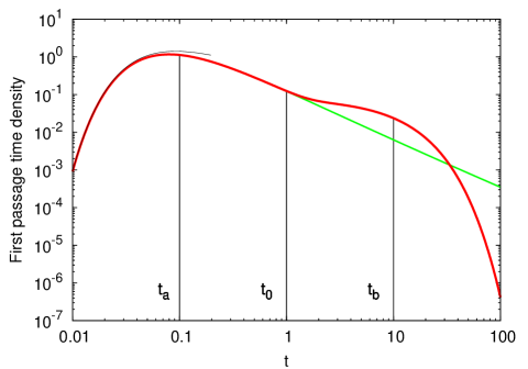
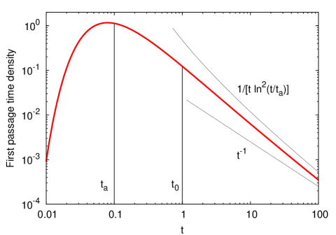
Figure 4: First passage time density $\wp(t)$. Left: The outer cylinder is present, eventually causing an exponential-like steep decay of $\wp(t)$, compared to the unbounded behavior. The black line shows the short time approximation (165). Right: Unbounded problem showing the long-time asymptotics. The inverse square-logarithmic term matters, as can be seen from comparison with the shown asymptotic behaviors.

VI.3 First passage time density at very short times $t\ll t_{a}$

We conclude our discussion of the first passage time density with the case of very short times, $t\ll t_{a}$. In this regime a particle starting close to the inner cylinder surface does not yet feel the cylindrical geometry and we would naively expect that the first passage is given by the one-dimensional Lévy-Smirnov form.

As we may neglect the outer cylinder, we start from result (149). We expand this result in inverse powers of $\sqrt{s}$ and then perform a term-wise inverse Laplace transform. With

$$K_{\nu}(z)=\sqrt{\frac{\pi}{2z}}e^{-z}\left\{1+\frac{4\nu^{2}-1}{8z}+\mathcal{O}\left(\frac{1}{z^{2}}\right)\right\},$$ (162)

we find that

$$\frac{K_{0}\left(\sqrt{st_{0}}\right)}{K_{0}\left(\sqrt{st_{a}}\right)} \sim \left(\frac{t_{a}}{t_{0}}\right)^{1/4}\exp\left(-\sqrt{s}\Big{[}\sqrt{t_{0}}-\sqrt{t_{a}}\Big{]}\right)$$ (163)

$$\times\left\{1+\frac{1}{8}\left(\frac{1}{\sqrt{st_{a}}}-\frac{1}{\sqrt{st_{0}}}\right)\right\}$$

$$\sim \left(\frac{a}{r_{0}}\right)^{1/2}\exp\left(-\sqrt{s}\frac{r_{0}-a}{\sqrt{D_{b}}}\right)$$

$$\times\left\{1+\frac{\sqrt{D_{b}}}{8\sqrt{s}}\frac{r_{0}-a}{ar_{0}}\right\}.$$

We are thus led to the inverse Laplace transform

$$\wp(t) \sim \left(\frac{a}{r_{0}}\right)^{1/2}\frac{r_{0}-a}{\sqrt{D_{b}}}\frac{1}{2\sqrt{\pi t^{3}}}\exp\left(-\frac{(r_{0}-a)^{2}}{4D_{b}t}\right)$$ (164)

$$+\left(\frac{a}{r_{0}}\right)^{1/2}\frac{r_{0}-a}{ar_{0}}\frac{\sqrt{D_{b}}}{8\sqrt{\pi t}}\exp\left(-\frac{(r_{0}-a)^{2}}{4D_{b}t}\right).$$

Reorganizing this expression we find

$$\wp(t) \sim \left(\frac{a}{r_{0}}\right)^{1/2}\frac{r_{0}-a}{\sqrt{4\pi D_{b}t^{3}}}\exp\left(-\frac{(r_{0}-a)^{2}}{4D_{b}t}\right)$$ (165)

$$\times\left\{1+\frac{D_{b}t}{4ar_{0}}+\ldots\right\}.$$

At very short times the first passage time density indeed coincides with the one-dimensional limit, reweighted by the ratio $\sqrt{a/r_{0}}$. Note that if we keep the distance $\Delta=r_{0}-a$ fixed but let both $r_{0}$ and $a$ tend to infinity, we recover the result for a flat surface,

$$\wp_{\mathrm{flat}}(t)=\frac{\Delta}{\sqrt{4\pi D_{b}t^{3}}}\exp\left(-\frac{\Delta^{2}}{4D_{b}t}\right),$$ (166)

i.e., the well-known Lévy-Smirnov distribution.

VII Discussion

We established an exact approach to BMSD along a reactive cylindrical surface revealing four distinct diffusion regimes. In particular our formalism provides a stringent derivation of the transient superdiffusion discussed earlier and explicitly quantifies the transition to other regimes. Notably we revealed a saturation regime for the MSD along the cylinder that becomes relevant at times above which the diffusing particle feels the curvature of the cylinder surface ($t_{a}$). This behavior, caused by the cylindrical geometry, stems from an interesting balance between a net flux of particles into the bulk and the fact that particles with a longer return time also lead to an increased effective surface relocation. In absence of an outer cylinder the saturation is terminal, while in its presence the MSD along the cylinder returns to a linear growth in time. This observation will be important in future models of BMSD around cylinders and particularly for the interpretation of experimental data obtained for BMSD systems. We note that in the proper limit $a\to\infty$ the previous results for a planar surface are recovered. Relaxing the strong coupling condition we demonstrated the existence of an almost ballistic BMSD behavior, a case that might be relevant for transport along thin cylinders such as DNA.

In Ref. levitz it was shown that the scaling behavior in the regimes below and above $t_{a}$ can be probed experimentally by NMR methods measuring the BMSD of water molecules along imogolite nanorods over three orders of magnitude in frequency space. For larger molecules such as a protein of approximate diameter 5 nm we observe a diffusivity of $10^{-6}\mathrm{cm}^{2}/\mathrm{sec}$ such that for instance the saturation plateau around a bacillus cell (radius 1/2 $\mu$m) sets in at around $t_{a}=2.5$ msec which might give rise to interesting consequences for the material exchange around such cells. In general, the relevance of the individual regimes will crucially depend on the scales of the surface radius and the diffusing particle (and therefore its diffusivity). It was discussed previously that even the superdiffusive short-term behavior may become relevant bychuk ; bychuk1 ; fatkullin . In general, in a given system the separation between the various scaling regimes may not be sharp. Moreover typically a single experimental technique will not be able to probe all regimes. It is therefore vital to have available a solution for the entire BMSD problem.

Appendix A Derivation of the reactive boundary condition for a planar surface

We start with a derivation of the coupling between surface and bulk in a discrete random walk process along the $\rho$ coordinate perpendicular to the surface, as specified in Fig. 5. Let $N_{i}$ with $i=1,2,\ldots$ denote the number of particles at site $i$ of this one-dimensional lattice with spacing $a$. The number of particles on the surface at lattice site $i=0$ are termed $\mathcal{N}_{0}$. The exchange of particles is possible only via nearest neighbor jumps, each characterized by the waiting time $\tau$. For the exchange between the surface and site $i=1$ we then have the following law

$$\frac{d\mathcal{N}_{0}(t)}{dt}=\frac{1}{2\tau}N_{1}-\frac{1}{\tau_{\mathrm{des}}}\mathcal{N}_{0},$$ (167)

where $\tau_{\mathrm{des}}$ is the characteristic time for desorption from the surface. The bulk sites are governed by equations of the form

$$\frac{dN_{1}(t)}{dt} = \frac{1}{\tau_{\mathrm{des}}}\mathcal{N}_{0}-\frac{1}{\tau}N_{1}+\frac{1}{2\tau}N_{2},$$

$$\frac{dN_{2}(t)}{dt} = \frac{1}{2\tau}N_{1}+\frac{1}{2\tau}N_{3}-\frac{1}{\tau}N_{2},$$ (168)

etc. Let us define the number of “bulk” particles at the surface site $i=0$ through

$$N_{0}\equiv\frac{2\tau}{\tau_{\mathrm{des}}}\mathcal{N}_{0}.$$ (169)

This trick will allows us to formulate the exchange equation also for site $i=1$ in a homogeneous form. Namely, from Eq. (167) we have

$$\frac{d\mathcal{N}_{0}(t)}{dt}=\frac{1}{2\tau}\left(N_{1}-N_{0}\right).$$ (170)

Moreover, from Eqs. (168) we find

$$\frac{dN_{1}(t)}{dt}=\frac{1}{2\tau}\left(N_{0}-2N_{1}+N_{2}\right),$$ (171)

and

$$\frac{dN_{2}(t)}{dt}=\frac{1}{2\tau}\left(N_{1}-2N_{2}+N_{3}\right),$$ (172)

etc.

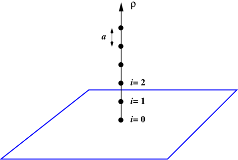
Figure 5: Schematic of the random walk picture of the surface-bulk exchange. In our derivation we pass from the discrete lattice with spacing $a$ to the continuous variable $\rho$. The surface corresponds to $\rho=0$.

Let us now take the continuum limit. For that purpose we make a transition from $\mathcal{N}_{0}\to n_{s}$ as the number of surface particles, and $N_{i}\to an_{b}$ for the bulk concentration of particles. Expansion of the right hand side of Eq. (170) yields the surface-bulk coupling

$$\frac{\partial n_{s}(t)}{\partial t}=\frac{a}{2\tau}a\left.\frac{\partial n_{b}(\rho,t)}{\partial\rho}\right|_{\rho=0}.$$ (173)

Similarly from Eq. (171) we obtain the bulk diffusion equation

$$\frac{\partial n_{b}(\rho,t)}{\partial t}=\frac{1}{2\tau}a^{2}\frac{\partial^{2}n_{b}}{\partial\rho^{2}}.$$ (174)

Finally, the boundary condition

$$\left.\frac{a}{2\tau}n_{b}(\rho,t)\right|_{\rho=0}=\frac{1}{\tau_{\mathrm{des}}}n_{s}$$ (175)

stems from our definition (169).

Appendix B Calculation of the surface mean squared displacement

To calculate the quantity (54) we start by rewriting expression (48) in the form

$$n(k,s)=\frac{N_{0}}{s+k^{2}D_{s}+A(q,s)},$$ (176)

where

$$q\equiv\sqrt{k^{2}+s/D_{b}}$$ (177)

and

$$A(q,s)=\kappa q\frac{\Delta_{1}(q,s)}{\Delta(q,s)}.$$ (178)

Differentiation of $n(k,s)$ yields

$$\frac{\partial}{\partial k}n(k,s)=-\frac{N_{0}}{\left(s+k^{2}D_{s}+A(q,s)\right)^{2}}\left(2kD_{s}+\frac{\partial A(q,s)}{\partial q}\frac{\partial q}{\partial k}\right),$$ (179)

and thus double differentiation of $n(k,s)$ produces

$$\frac{\partial^{2}}{\partial k^{2}}n(k,s) = -\frac{N_{0}}{\left(s+k^{2}D_{s}+A(q,s)\right)^{2}}\left(2D_{s}+\frac{\partial^{2}A(q,s)}{\partial k^{2}}\right)$$ (180)

$$+\frac{2N_{0}}{\left(s+k^{2}D_{s}+A(q,s)\right)^{3}}\left(2kD_{s}+\frac{\partial A}{\partial k}\right)^{2}.$$

Since

$$\left.\frac{\partial q}{\partial k}\right|_{k=0}=0,$$ (181)

and therefore

$$\left.\frac{\partial A(q,s)}{\partial k}\right|_{k=0}=0\,\,\,\mbox{and}\,\,\,\left.\frac{\partial n(k,s)}{\partial k}\right|_{k=0}=0,$$ (182)

such that the first moment $\langle z(t)\rangle$ of $n(z,t)$ vanishes, as it should due to symmetry reasons. Moreover, we then obtain

$$\langle z^{2}(s)\rangle = \frac{1}{\left[s+A(0,s)\right]^{2}}\left[2D_{s}+\left.\frac{\partial^{2}A}{\partial k^{2}}\right|_{k=0}\right]$$ (183)

$$= \frac{N_{s}^{2}(s)}{N_{0}^{2}}\left[2D_{s}+\left.\frac{\partial^{2}A}{\partial k^{2}}\right|_{k=0}\right].$$

The second term in the square brackets can be transformed to

$$\frac{\partial^{2}A(q,s)}{\partial k^{2}}=\frac{\partial}{\partial k}\left(\frac{\partial A(q,s)}{\partial q}\right)\frac{\partial q}{\partial k}+\frac{\partial A(q,s)}{\partial q}\frac{\partial^{2}q}{\partial k^{2}},$$ (184)

such that

$$\left.\frac{\partial^{2}A(q,s)}{\partial k^{2}}\right|_{k=0}=\sqrt{\frac{D_{b}}{s}}\left.\frac{\partial A(q,s)}{\partial q}\right|_{k=0}.$$ (185)

Differentiation of $A(q,s)$ results in the expression

$$\frac{\partial A(q,s)}{\partial q}=\kappa\frac{\Delta_{1}}{\Delta}\left[1+\frac{q}{\Delta_{1}}\frac{\partial\Delta_{1}}{\partial q}-\frac{q}{\Delta}\frac{\partial\Delta}{\partial q}\right].$$ (186)

At $k=0$ we have $q=\sqrt{s/D_{b}}$, and we ultimately obtain

$$\langle z^{2}(s)\rangle=\frac{N_{s}^{2}(s)}{N_{0}^{2}}\left\{2D_{s}+\kappa\sqrt{\frac{D_{b}}{s}}\frac{\Delta_{1}(0,s)}{\Delta(0,s)}\left[1+\sqrt{\frac{s}{D_{b}}}\left(\frac{1}{\Delta_{1}(0,s)}\left.\frac{\partial\Delta_{1}}{\partial q}\right|_{k=0}-\frac{1}{\Delta(0,s)}\left.\frac{\partial\Delta}{\partial q}\right|_{k=0}\right)\right]\right\}.$$ (187)

Here, we include the auxiliary quantities

$$\left.\frac{\partial\Delta_{1}}{\partial q}\right|_{k=0}=a\Big{[}K_{1}^{\prime}\left(\sqrt{st_{a}}\right)I_{1}\left(\sqrt{st_{b}}\right)-I_{1}^{\prime}\left(\sqrt{st_{a}}\right)K_{1}\left(\sqrt{st_{b}}\right)\Big{]}+b\Big{[}K_{1}\left(\sqrt{st_{a}}\right)I_{1}^{\prime}\left(\sqrt{st_{b}}\right)-I_{1}\left(\sqrt{st_{a}}\right)K_{1}^{\prime}\left(\sqrt{st_{b}}\right)\Big{]},$$ (188)

and

$$\left.\frac{\partial\Delta}{\partial q}\right|_{k=0}=a\Big{[}I_{1}\left(\sqrt{st_{a}}\right)K_{1}\left(\sqrt{st_{b}}\right)-K_{1}\left(\sqrt{st_{a}}\right)I_{1}\left(\sqrt{st_{b}}\right)\Big{]}+b\Big{[}I_{0}\left(\sqrt{st_{a}}\right)K_{1}^{\prime}\left(\sqrt{st_{b}}\right)+K_{0}\left(\sqrt{st_{a}}\right)I_{1}^{\prime}\left(\sqrt{st_{b}}\right)\Big{]},$$ (189)

In these expressions the prime implies a derivative over the whole argument, and we have abramowitz

$$I_{1}^{\prime}(z)=I_{0}(z)-\frac{1}{z}I_{1}(z),\,\,\,\mbox{and}\,\,\,K_{1}^{\prime}(z)=-K_{0}(z)-\frac{1}{z}K_{1}(z).$$ (190)

Taking the various limits corresponding to the cases discussed in Sections IV and V from above exact results we can indeed confirm the results obtained there based on the limiting forms for the surface propagator. We here demonstrate the corresponding derivations for the surface mean squared displacement based on the exact Eq. (187) in the strong binding regime.

(i) At short times $t\ll t_{\kappa}\ll t_{a}\ll t_{b}$ we use the expansions abramowitz

$$I_{\nu}(z)\sim\frac{e^{z}}{\sqrt{2\pi z}},\,\,\,\mbox{and}\,\,\,K_{\nu}(z)\sim\sqrt{\frac{\pi}{2z}}e^{-z}.$$ (191)

Moreover, with Eq. (190) we find that

$$I_{1}^{\prime}\left(\sqrt{st_{a/b}}\right)\sim I_{0}\left(\sqrt{st_{a/b}}\right)\sim\frac{\exp\left(\sqrt{st_{a/b}}\right)}{(2\pi)^{1/2}\left(st_{a/b}\right)^{1/4}}$$ (192)

and

$$K_{1}^{\prime}\left(\sqrt{st_{a/b}}\right)\sim-K_{0}\left(\sqrt{st_{a/b}}\right)\sim-\frac{\pi^{1/2}\exp\left(-\sqrt{st_{a/b}}\right)}{2^{1/2}\left(st_{a/b}\right)^{1/4}}$$ (193)

so that in this approximation

$$\Delta_{1}(0,s)\sim\Delta(0,s)\sim\frac{\exp\left(s^{1/2}\left[t_{b}^{1/2}-t_{a}^{1/2}\right]\right)}{2\left(st_{a}\right)^{1/4}\left(st_{b}\right)^{1/4}},$$ (194)

thus

$$\left.\frac{\partial\Delta_{1}}{\partial q}\right|_{k=0}\sim\left.\frac{\partial\Delta}{\partial q}\right|_{k=0}\sim(b-a)\frac{\exp\left(s^{1/2}\left[t_{b}^{1/2}-t_{a}^{1/2}\right]\right)}{2(st_{a})^{1/4}(st_{b})^{1/4}},$$ (195)

and finally

$$\left(\frac{1}{\Delta_{1}}\frac{\partial\Delta_{1}}{\partial q}-\frac{1}{\Delta}\frac{\partial\Delta}{\partial q}\right)_{k=0}\sim 0.$$ (196)

From expressions (187) and (64) we therefore obtain

$$\langle z^{2}(s)\rangle=\frac{2D_{s}}{s^{2}}+\frac{D_{b}}{s^{5/2}t_{\kappa}^{1/2}}.$$ (197)

With the Laplace transform pair

$$\frac{1}{s^{k}}\div\frac{t^{k-1}}{\Gamma(k)},\,\,\,k>0,$$ (198)

and $\Gamma(5/2)=3\pi^{1/2}/4$ we arrive at the result

$$\langle z^{2}(t)\rangle\sim 2D_{s}t\left[1+\frac{2D_{b}}{3\pi^{1/2}D_{s}}\left(\frac{t}{t_{\kappa}}\right)^{1/2}\right],$$ (199)

where the equivalence with the normalized mean squared displacement is due to the fact that $N_{s}(t)\sim N_{0}$ in this short time regime. This result coincides with our finding (68) obtained from the approximated surface propagator.

(ii) At intermediate times $t_{\kappa}\ll t\ll t_{a}\ll t_{b}$ approximation (196) still holds. From Eq. (187) and with the time evolution (85) of the number of particle on the surface in this regime, we obtain

$$\langle z^{2}(s)\rangle \sim \frac{N_{s}(s)^{2}}{N_{0}^{2}}\left[2D_{s}+\kappa\left(\frac{D_{b}}{s}\right)^{1/2}\right]$$ (200)

$$\sim 2D_{s}\frac{t_{\kappa}}{s}+D_{b}\frac{t_{\kappa}^{1/2}}{s^{3/2}},$$

and, after inverse Laplace transformation,

$$\langle z^{2}(t)\rangle\sim 2D_{s}t_{\kappa}+\frac{2D_{b}}{\pi^{1/2}}t_{\kappa}^{1/2}t^{1/2}.$$ (201)

Again, we find coincidence with the previous result (88).

(iii) At even longer times $t_{\kappa}\ll t_{a}\ll t\ll t_{b}$ we make use of approximations (113) and (191) to (193). For the derivatives of the Bessel functions we have in this regime

$$I_{1}^{\prime}\left(\sqrt{st_{a}}\right) = I_{0}\left(\sqrt{st_{a}}\right)-\frac{1}{\sqrt{st_{a}}}I_{1}\left(\sqrt{st_{a}}\right)\sim\frac{1}{2},$$

$$K_{1}^{\prime}\left(\sqrt{st_{a}}\right) = -K_{0}\left(\sqrt{st_{a}}\right)-\frac{1}{\sqrt{st_{a}}}K_{1}\left(\sqrt{st_{a}}\right)\sim-\frac{1}{st_{a}},$$

$$I_{1}^{\prime}\left(\sqrt{st_{b}}\right) \sim I_{0}\left(\sqrt{st_{b}}\right)\sim\frac{\exp\left(\left[st_{b}\right]^{1/2}\right)}{(2\pi)^{1/2}(st_{b})^{1/4}},$$

$$K_{1}^{\prime}\left(\sqrt{st_{b}}\right) \sim -K_{0}\left(\sqrt{st_{b}}\right)\sim-\frac{\pi^{1/2}\exp\left(-[st_{b}]^{1/2}\right)}{2^{1/2}(st_{b})^{1/4}}.$$ (202)

Therefore,

$$\Delta_{1}(0,s)\sim\frac{\exp\left([st_{b}]^{1/2}\right)}{(2\pi)^{1/2}(st_{a})^{1/2}(st_{b})^{1/4}}$$ (203)

and

$$\left.\frac{\partial\Delta_{1}}{\partial q}\right|_{k=0}=\left(\frac{b}{(st_{a})^{1/2}}-\frac{a}{st_{a}}\right)\frac{b\exp\left((st_{b})^{1/2}\right)}{(2\pi)^{1/2}(st_{b})^{1/4}},$$ (204)

as well as

$$\Delta(0,s)\sim\frac{1}{2}\frac{\exp\left([st_{b}]^{1/2}\right)}{(2\pi)^{1/2}(st_{b})^{1/4}}\ln\left(\frac{4}{C^{2}st_{a}}\right)$$ (205)

and

$$\left.\frac{\partial\Delta}{\partial q}\right|_{k=0}=\left[-\frac{a}{(st_{a})^{1/2}}+\frac{b}{2}\ln\left(\frac{4}{C^{2}st_{a}}\right)\right]\frac{\exp\left((st_{b})^{1/2}\right)}{(2\pi)^{1/2}(st_{b})^{1/4}}.$$ (206)

Here we define $C=\exp(\gamma)\approx 1.78107$, where $\gamma\approx 0.577216$ is Euler’s $\gamma$ constant. Collecting our results we find that

$$\left.\frac{1}{\Delta_{1}(0,s)}\frac{\partial\Delta_{1}}{\partial q}\right|_{k=0}-\left.\frac{1}{\Delta(0,s)}\frac{\partial\Delta}{\partial q}\right|_{k=0}$$

$$\hskip 34.14322pt\sim\frac{a}{(st_{a})^{1/2}}\left(-1+\frac{2}{\displaystyle\ln\left(\frac{4}{C^{2}st_{a}}\right)}\right)$$ (207)

and ultimately recover

$$\langle z^{2}(s)\rangle\sim\frac{N_{s}(s)^{2}}{N_{0}^{2}}\left[2D_{s}+\frac{4D_{b}}{(t_{a}t_{\kappa})^{1/2}}\frac{1}{\displaystyle s\ln^{2}\left(\frac{4}{C^{2}st_{a}}\right)}\right].$$ (208)

Inserting expression (98) we obtain

$$\langle z^{2}(s)\rangle\sim\frac{D_{s}t_{a}t_{\kappa}}{2}\ln^{2}\left(\frac{4}{C^{2}st_{a}}\right)+\frac{D_{b}(t_{a}t_{\kappa})^{1/2}}{s}.$$ (209)

By Tauberian theorems the final result for the surface mean squared displacements in this long time regime are

$$\langle z^{2}(t)\rangle\sim\frac{D_{s}t_{a}t_{\kappa}}{t}\ln\left(\frac{4t}{Ct_{a}}\right)+D_{b}(t_{a}t_{\kappa})^{1/2}.$$ (210)

This result corroborates Eq. (104).

(iv) Finally, at very long times $t_{\kappa}\ll t_{a}\ll t_{b}\ll t$ we have the asymptotic behaviors

$$I_{0}\left(\sqrt{st_{a/b}}\right) \sim 1,$$

$$K_{0}\left(\sqrt{st_{a/b}}\right) \sim -\gamma-\ln\left(\frac{(st_{a/b})^{1/2}}{2}\right),$$

$$I_{1}\left(\sqrt{st_{a/b}}\right) \sim \frac{1}{2}(st_{a/b})^{1/2},$$

$$K_{1}\left(\sqrt{st_{a/b}}\right) \sim (st_{a/b})^{-1/2},$$

$$I_{1}^{\prime}\left(\sqrt{st_{a/b}}\right) = I_{0}\left(\sqrt{st_{a/b}}\right)-\frac{I_{1}\left(\sqrt{st_{a/b}}\right)}{(st_{a/b})^{1/2}}\sim\frac{1}{2},$$

$$K_{1}^{\prime}\left(\sqrt{st_{a/b}}\right) = -K_{0}\left(\sqrt{st_{a/b}}\right)-\frac{K_{1}\left(\sqrt{st_{a/b}}\right)}{(st_{a/b})^{1/2}}$$ (211)

$$\sim -\frac{1}{st_{a/b}}.$$

Therefore,

$$\left.\frac{\partial\Delta_{1}}{\partial q}\right|_{k=0}\sim\frac{b}{4}(st_{a})^{1/2}\ln\left(\frac{4}{C^{2}st_{a}}\right)$$ (212)

and

$$\Delta_{1}(0,s)\sim\frac{1}{2}\sqrt{\frac{t_{b}}{t_{a}}}$$ (213)

as well as

$$\left.\frac{\partial\Delta}{\partial q}\right|_{k=0}\sim-\frac{b}{st_{b}}+\frac{b}{4}\ln\left(\frac{4}{C^{2}st_{a}}\right)$$ (214)

and

$$\Delta(0,s)\sim\frac{1}{(st_{b})^{1/2}}.$$ (215)

For the square bracket in expression (187) we obtain

$$\Big{[}1+\ldots\Big{]}\sim 2,$$ (216)

and thus

$$\langle z^{2}(s)\rangle\sim\frac{N_{s}^{2}(s)}{N_{0}^{2}}\left[2D_{s}+D_{b}\frac{t_{b}}{(t_{a}t_{\kappa})^{1/2}}\right].$$ (217)

With the help of Eq. (115) this implies the result for the surface mean squared displacement

$$\langle z^{2}(t)\rangle\sim\frac{8t_{a}t_{\kappa}}{t_{b}^{2}}D_{s}t+\frac{4(t_{a}t_{\kappa})^{1/2}}{t_{b}}D_{b}t.$$ (218)

Thus, we corroborate the finding (121) from the approximate calculation. With similar calculations one can reproduce the time evolution of the number of particles on the inner cylinder surface and thus the normalized surface mean squared displacement. Analogous reasoning confirms the results obtained for the intermediate coupling limit in Sec. V.

Appendix C Calculation of the first passage time density

In the Fourier-Laplace domain the diffusion equation (144) becomes an ordinary differential equation,

$$\frac{d^{2}}{dr^{2}}P(r,k,s)+\frac{1}{r}\frac{d}{dr}P(r,k,s)-q^{2}P(r,k,s)$$

$$\hskip 102.43008pt=-\frac{\delta(r-r_{0})}{2\pi r_{0}D_{b}},$$ (219)

where

$$q^{2}=k^{2}+\frac{s}{D_{b}}.$$ (220)

The boundary conditions are

$$P(r,k,s)\Big{|}_{r=a}=0$$ (221)

and

$$\left.\frac{\partial}{\partial r}P(r,k,s)\right|_{r=b}=0.$$ (222)

We rewrite the Fourier-Laplace transformed diffusion equation (219) in the form

$$\mathbb{L}P(r,k,s)=\phi(r)$$ (223)

where the operator $\mathbb{L}$ and the inhomogeneity $\phi(r)$ represent

$$\mathbb{L}=\frac{d^{2}}{dr^{2}}+\frac{1}{r}\frac{d}{dr}-q^{2}$$ (224)

and

$$\phi(r)=\frac{\delta(r-r_{0})}{2\pi r_{0}D_{b}}.$$ (225)

Eq. (223) can be solved by the method of variation of coefficients. Namely, knowing that the solution of the homogeneous equation reads

$$P(r,k,s)=AI_{0}(qr)+BK_{0}(qr),$$ (226)

to solve the full equation we assume that $A$ and $B$ are some functions of the radius $r$. We impose the condition

$$A^{\prime}(r)I_{0}(qr)+B^{\prime}(r)K_{0}(qr)=0,$$ (227)

where the prime denotes a derivative with respect to $r$. Consequently we find

$$P^{\prime}(r,k,s)=A(r)I_{0}^{\prime}(qr)+B(r)K_{0}^{\prime}(qr),$$ (228)

and

$$P^{\prime\prime}(r,k,s) = A(r)I_{0}^{\prime\prime}(qr)+B(r)K_{0}^{\prime\prime}(qr)$$ (229)

$$+A^{\prime}(r)I_{0}^{\prime}(qr)+B^{\prime}(r)K_{0}^{\prime}(qr).$$

According to the method of variation of coefficients this leads to

$$\mathbb{L}P(r,k,s)=A^{\prime}(r)I_{0}^{\prime}(qr)+B^{\prime}(r)K_{0}^{\prime}(qr).$$ (230)

With above relations we arrive at a system of two equations with two unknowns, $A^{\prime}$ and $B^{\prime}$,

$$A^{\prime}(r)I_{0}(qr)+B^{\prime}(r)K_{0}(qr)=0$$

$$A^{\prime}(r)I_{0}^{\prime}(qr)+B^{\prime}(r)K_{0}^{\prime}(qr)=\phi(r),$$ (231)

The corresponding Wronskian is abramowitz

$$W(r) = I_{0}(qr)K_{0}^{\prime}(qr)-K_{0}(qr)I_{0}^{\prime}(qr)$$ (232)

$$= -q\Big{(}I_{0}(qr)K_{1}(qr)+I_{1}(qr)K_{0}(qr)\Big{)}$$

$$= -\frac{1}{r}.$$

The solutions to Eqs. (231) is

$$A^{\prime}(r)=-\frac{1}{W(r)}K_{0}(qr)\phi(r)$$ (233)

and

$$B^{\prime}(r)=\frac{1}{W(r)}I_{0}(qr)\phi(r),$$ (234)

and thus

$$A(r) = -\int\frac{1}{W(r)}K_{0}(qr)\phi(r)dr$$

$$B(r) = \int\frac{1}{W(r)}I_{0}(qr)\phi(r)dr.$$ (235)

The general solution of Eq. (223) has the form

$$P(r,k,s) = \left(-\int\frac{1}{W(r)}K_{0}(qr)\phi(r)dr+A_{0}\right)I_{0}(qr)$$ (236)

$$+\left(\int\frac{1}{W(r)}I_{0}(qr)\phi(r)dr+B_{0}\right)K_{0}(qr),$$

where the constants $A_{0}$ and $B_{0}$ are determined by the boundary conditions that are rewritten as

$$P(a,k,s)=\lim_{r\to a^{+}}\left\{\left(-\int_{a}^{r}\frac{1}{W(r^{\prime})}K_{0}(qr^{\prime})\phi(r^{\prime})dr^{\prime}+A_{0}\right)I_{0}(qr)+\left(\int_{a}^{r}\frac{1}{W(r^{\prime})}I_{0}(qr^{\prime})\phi(r^{\prime})dr^{\prime}+B_{0}\right)K_{0}(qr)\right\}=0$$ (237)

and

$$\left.\frac{\partial}{\partial r}P(r,k,s)\right|_{r=b}=\left(-\int_{a}^{b}\frac{1}{W(r^{\prime})}K_{0}(qr^{\prime})\phi(r^{\prime})dr^{\prime}+A_{0}\right)qI_{0}^{\prime}(qb)+\left(\int_{a}^{b}\frac{1}{W(r^{\prime})}I_{0}(qr^{\prime})\phi(r^{\prime})dr^{\prime}+B_{0}\right)qK_{0}^{\prime}(qb)=0.$$ (238)

Since the inhomogeneity $\phi(r)$ is a $\delta$ distribution, in general we have to consider two cases separately: $r<r_{0}$ and $r>r_{0}$. However, as we are interested solely in the first passage problem, for which we require the probability flow at $r=a<r_{0}$ we restrict ourselves to the former case, only. This means that Eq. (237) simplifies to

$$A_{0}I_{0}(qa)+B_{0}K_{0}(qa)=0.$$ (239)

Performing the integrals in expression (238) and using Eq. (231) we obtain the following system to determine the constants $A_{0}$ and $B_{0}$:

$$A_{0}I_{0}(qa)+B_{0}K_{0}(qa)=0$$

$$A_{0}qI_{1}(qb)-B_{0}qK_{1}(qb)=\frac{q}{2\pi D_{b}}\Big{(}I_{1}(qb)K_{0}(qr_{0})$$

$$\hskip 119.50148pt+K_{1}(qb)I_{0}(qr_{0})\Big{)}$$ (240)

with the following determinant

$$\mathrm{det}=-q\Big{(}I_{0}(qa)K_{1}(qb)+K_{0}(qa)I_{1}(qb)\Big{)}.$$ (241)

The solution of Eq. (240) is then

$$A_{0}=\frac{K_{0}(qa)}{2\pi D_{b}}\frac{I_{1}(qb)K_{0}(qr_{0})+K_{1}(qb)I_{0}(qr_{0})}{I_{0}(qa)K_{1}(qb)+K_{0}(qa)I_{1}(qb)}$$ (242)

and

$$B_{0}=-\frac{I_{0}(qa)}{2\pi D_{b}}\frac{I_{1}(qb)K_{0}(qr_{0})+K_{1}(qb)I_{0}(qr_{0})}{I_{0}(qa)K_{1}(qb)+K_{0}(qa)I_{1}(qb)}.$$ (243)

These two relations introduced into Eq. (236) we obtain

$$P(r,k,s)=\frac{1}{2\pi D_{b}}\frac{I_{1}(qb)K_{0}(qr_{0})+K_{1}(qb)I_{0}(qr_{0})}{I_{0}(qa)K_{1}(qb)+K_{0}(qa)I_{1}(qb)}\Big{(}K_{0}(qa)I_{0}(qr)-I_{0}(qa)K_{0}(qr)\Big{)},\,\,\,r\leq r_{0}.$$ (244)

This result coincides with the findings of Berg and Blomberg berg , when one takes the limit of a completely absorbing boundary condition [in Berg and Blomberg’s notation, this corresponds to $k\to\infty$ of their reaction rate $k$].

Appendix D Some Laplace transforms

We here provide a summary of non-trivial Laplace transforms involving logarithmic functions, used throughout the text.

D.1 Laplace inversion of the logarithm

To calculate the inverse Laplace transforms in Eqs. (98) and (99), as well as (109) and (110), we use the direct Laplace transform of $\ln t$. Namely, for some $A>0$,

$$\mathscr{L}\left\{\ln\left(\frac{t}{A}\right)\right\}=\int_{0}^{\infty}e^{-st}\ln\left(\frac{t}{A}\right)dt=-\frac{1}{s}\Big{(}\gamma+\ln(As)\Big{)},$$ (245)

where $\gamma=-\int_{0}^{\infty}\exp(-x)\ln xdx\approx 0.5772$ is Euler’s constant. Introducing the Laplace inversion with appropriate Bromwich path, we obtain

$$\int_{\mathrm{Br}}e^{st}\frac{\ln(As)}{s}\frac{ds}{2\pi i}=-\ln\left(\frac{Ct}{A}\right),$$ (246)

where $C=\exp(\gamma)$. Differentiation of this result with respect to $t$ yields

$$\int_{\mathrm{Br}}e^{st}\ln(As)\frac{ds}{2\pi i}=-\frac{1}{t},$$ (247)

which is an exact result.

Eq. (247) delivers the desired result for Eq. (99):

$$\mathscr{L}^{-1}\left\{\ln\left(\frac{4}{C^{2}st_{a}}\right)\right\}=\frac{1}{t},$$ (248)

and for Eq. (110):

$$\mathscr{L}^{-1}\left\{\ln\Big{(}st_{a}+k^{2}a^{2}\Big{)}\right\}=-\frac{1}{t}e^{-k^{2}a^{2}t/t_{a}}.$$ (249)

For the latter relation we used the shift theorem of the Laplace transform:

$$\int_{\mathrm{Br}}e^{st}\ln(s+\Delta)\frac{ds}{2\pi i}=-\frac{1}{t}e^{\Delta t}.$$ (250)

D.2 Laplace inversion of the squared logarithm

To obtain the Laplace pair (103) we calculate

$$\int_{\mathrm{Br}}e^{st}\Big{[}\ln(As)\Big{]}^{2}\frac{ds}{2\pi i},\,\,\,A>0.$$ (251)

We first deform the Bromwich path into the Hankel path $\mathrm{Ha}(\epsilon)$, that is a loop starting from $-\infty$ below the negative real axis, merging into a small circle around the origin with radius $|s|=\epsilon$, with $\epsilon\to 0$ in a positive sense, and finally receding to $-\infty$ moving above the negative real axis. The integral along the Hankel path can be evaluated directly:

$$I = \int_{\mathrm{Br}}e^{st}\Big{[}\ln(As)\Big{]}^{2}\frac{ds}{2\pi i}=\int_{\mathrm{Ha}(\epsilon)}e^{st}\Big{[}\ln(As)\Big{]}^{2}\frac{ds}{2\pi i}$$ (252)

$$= \int_{-\infty}^{0}\exp\left(|s|te^{-i\pi}\right)\Big{[}\ln\left(A|s|e^{-i\pi}\right)\Big{]}^{2}\frac{d|s|\exp(-i\pi)}{2\pi i}+\int_{0}^{\infty}\exp\left(|s|te^{i\pi}\right)\Big{[}\ln\left(A|s|e^{i\pi}\right)\Big{]}^{2}\frac{d|s|\exp(i\pi)}{2\pi i}+I_{\epsilon}.$$

Here $I_{\epsilon}\to 0$ at $\epsilon\to 0$ is the integral over the small circle of radius $\epsilon$ around the origin. Collecting the terms we find

$$I=\int_{0}^{\infty}e^{-st}\Big{[}\ln(As)-i\pi\Big{]}^{2}\frac{ds}{2\pi i}+c.c=-2\int_{0}^{\infty}e^{-st}\ln(As)ds,$$ (253)

so that we finally obtain

$$\int_{\mathrm{Br}}e^{st}\Big{[}\ln(As)\Big{]}^{2}\frac{ds}{2\pi i}=\frac{2}{t}\ln\left(\frac{Ct}{A}\right).$$ (254)

Thus, we find Eq. (103),

$$\mathscr{L}^{-1}\left\{\ln^{2}\left(\frac{C^{2}t_{a}}{4}s\right)\right\}=\frac{2}{t}\ln\left(\frac{4t}{Ct_{a}}\right).$$ (255)

D.3 Laplace inversion of the inverse square logarithm with additional power

We now address the Laplace pair of Eqs. (140) and (141), namely,

$$\mathscr{L}^{-1}\left\{s^{-3}\ln^{-2}\left(\frac{4}{C^{2}st_{a}}\right)\right\}=\frac{t^{2}}{2}\ln^{-2}\left(\frac{4t}{C^{2}t_{a}}\right).$$ (256)

To see this result let us recall the Tauberian theorems, see, for instance, Ref. feller . These state that if the Laplace transform of some (positive) function $\omega(t)$ behaves like

$$\omega(s)\sim s^{-\rho}L\left(\frac{1}{s}\right),\,\,\,s\to 0,\,\,\,0\leq\rho<\infty,$$ (257)

then its inverse Laplace transform has the asymptotic form

$$\omega(t)\sim\frac{t^{\rho-1}}{\Gamma(\rho)}L(t),\,\,\,t\to\infty.$$ (258)

Here $L(t)$ is a function slowly varying at infinity, i.e.,

$$\lim_{x\to\infty}\frac{L(ax)}{L(x)}=1\,\,\,\forall\,\,\,a>0.$$ (259)

References

• (1) O. V. Bychuk and B. O’Shaughnessy, Phys. Rev. Lett. 74, 1795 (1995).
• (2) O. V. Bychuk and B. O’Shaugnessy, J. Chem. Phys. 101, 772 (1994).
• (3) J. A. Revelli, C. E. Budde, D. Prato, and H. S. Wio, New J. Phys. 7, 16 (2005).
• (4) R. Valiullin, R. Kimmich, and N. Fatkullin, Phys. Rev. E 56, 4371 (1997).
• (5) P. Levitz, M. Zinsmeister, P. Davidson, D. Constantin, and O. Poncelet, Phys. Rev. E 78, 030102(R) (2008).
• (6) A. V. Chechkin, I. M. Zaid, M. A. Lomholt, I. M. Sokolov, and R. Metzler, Phys. Rev. E 79 040105(R) (2009).
• (7) R. Metzler and J. Klafter, Phys. Rep. 339, 1 (2000); J. Phys. A 37, R161 (2004).
• (8) J. Klafter and I. M. Sokolov, Phys. World 18, 29 (2005).
• (9) R. Kimmich, S. Stapf, P. Callaghan, and A. Coy, Magnet. Reson. Imaging 12, 339 (1994).
• (10) S. Stapf, R. Kimmich and R.-O. Seitter, Phys. Rev. Lett. 75, 2855 (1995).
• (11) M. V. Velosoa, A.G. Souza Filhoa, J. Mendes Filhoa, and Solange B. Faganb, Chem. Phys. Lett. 430, 71 (2006).
• (12) P.H. von Hippel and O.G. Berg, J. Biol. Chem. 264, 675 (1989); O. G. Berg and M. Ehrenberg, Biophys. Chem. 15, 41 (1982); M. A. Lomholt, B. v. d. Broek, S.-M. J. Kalisch, G. J. L. Wuite, and R. Metzler, Proc. Natl. Acad. Sci. USA 106, 8204 (2009).
• (13) O. G. Berg and C. Blomberg, Biophys. Chem. 4, 367 (1976).
• (14) I. Bonnet, A. Biebricher, P.-L. Porté, C. Loverdo, O. Bénichou, R. Voituriez, C. Escudé, W. Wende, A. Pingoud, and P. Desbiolles, Nucl. Acids Res. 36, 4118 (2008); I. M. Sokolov, R. Metzler, K. Pant, and M. C. Williams, Biophys. J. 89, 895 (2005); B. v. d. Broek, M. A. Lomholt, S.-M. J. Kalisch, R. Metzler, and G. J. L. Wuite, Proc. Natl. Acad. Sci. USA 105, 15738 (2008).
• (15) Y. M. Wang, R. H. Austin, and E. C. Cox, Phys. Rev. Lett. 97, 048302 (2006).
• (16) C. Bustamante, Y. R. Chemla, N. R. Forde, and D. Izhaky, Ann. Rev. Biochem. 73 705 (2004).
• (17) S. I. Coyne and N. H. Mendelson, Infection and Immunity 12, 1189 (1975).
• (18) M. A. Lomholt, I. M. Zaid, and R. Metzler, Phys. Rev. Lett. 98, 200603 (2007); I. M. Zaid, M. A. Lomholt, and R. Metzler, Biophys. J. 97, 710 (2009).
• (19) R. B. Winter, O. G. Berg, and P. H. von Hippel, Biochem. 20, 6961 (1981).
• (20) A. V. Chechkin, V. Yu. Gonchar, J. Klafter, R. Metzler, and L. V. Tanatarov, J. Stat. Phys. 115, 1505 (2004).
• (21) S. G. Samko, A. A. Kilbas, and O. I. Marichev, Fractional Integrals and Derivatives, Theory and Applications (Gordon and Breach, New York, NY 1993)
• (22) Substituting $x^{2}+z^{2}$ for $r^{2}$ in Eq. (6) of Ref. bychuk1 and integrating $x$ over $(-\infty,\infty)$ produces Eq. (70).
• (23) R. Metzler and J. Klafter, Europhys. Lett. 51, 492 (2000).
• (24) R. Gorenflo and F. Mainardi, in A. Carpinteri and F. Mainardi, Editors, Fractals and Fractional Calculus in Continuum Mechanics (Springer-Verlag, New York, 1997), pp. 223-276.
• (25) I. Podlubny, Fractional differential equations (Academic Press, San Diego, CA, 1998).
• (26) F. Mainardi, Y. Luchko, and G. Pagnini, Fract. Calc. Appl. Anal. 4, 153 (2001); Y. Luchko and R. Gorenflo, Fract. Calc. Appl. Anal. 1, 63 (1998); B. J. West and T. F. Nonnenmacher, Phys. Lett. A 278, 255 (2001).
• (27) R. Metzler and T. F. Nonnenmacher, Chem. Phys. 284, 67 (2002).
• (28) F. Mainardi, in A. Carpinteri and F. Mainardi, Editors, Fractals and Fractional Calculus in Continuum Mechanics (Springer-Verlag, New York, 1997), pp. 291-348.
• (29) In our problem we deal with a truncated Cauchy distribution, therefore the normalization factor in Eq. (70) is actually different from $1/\pi$. However, as the truncation is accomplished by the rapidly decaying compressed Gaussian, the correction to $1/\pi$ is expected to be small, and the Cauchy part contains almost the entire probability,
$$\frac{2}{\pi}\int_{0}^{\sqrt{D_{b}t}}\frac{\kappa t}{z^{2}+\kappa^{2}t^{2}}dz=\frac{2}{\pi}\arctan\sqrt{\frac{t_{\kappa}}{t}}\approx 1,$$
since $t\ll t_{\kappa}$.
• (30) M. Abramowitz and I. Stegun, Handbook of Mathematical Functions (Dover, New York NY, 1972)
• (31) S. Havlin and G. H. Weiss, J. Stat. Phys. 58, 1267 (1990).
• (32) W. Feller, An introduction to probability theory and its applications (John Wiley & Sons, New York, NY, 1968), Vol. II, Chapter XIII, Eqs. (5.15) and (5.17).