Optimal estimation of entanglement in optical qubit systems

Abstract

We address the experimental determination of entanglement for systems made of a pair of polarization qubits. We exploit quantum estimation theory to derive optimal estimators, which are then implemented to achieve ultimate bound to precision. In particular, we present a set of experiments aimed at measuring the amount of entanglement for states belonging to different families of pure and mixed two-qubit two-photon states. Our scheme is based on visibility measurements of quantum correlations and achieves the ultimate precision allowed by quantum mechanics in the limit of Poissonian distribution of coincidence counts. Although optimal estimation of entanglement does not require the full tomography of the states we have also performed state reconstruction using two different sets of tomographic projectors and explicitly shown that they provide a less precise determination of entanglement. The use of optimal estimators also allows us to compare and statistically assess the different noise models used to describe decoherence effects occuring in the generation of entanglement.

I Introduction

The sort of quantum correlations captured by the notion of entanglement represents a central resource for quantum information processing. Therefore, the precise characterization of entangled states is a crucial issue for the development of quantum technologies. In fact, quantification and detection of entanglement have been extensively investigated, see ren1 ; ren2 ; ren3 for a review, and different approaches have been developed to extract the amount of entanglement of a state from a given set of measurement results bayE ; Wun09 ; Eis07 ; KA06 . Of course, in order to evaluate the entanglement of a quantum state one may resort to full quantum state tomography LNP that, however, becomes impractical in higher dimensions and may be affected by large uncertainty TE94 ; AS2011 . Other methods, requiring a reduced number of observables, are based on visibility measurements Jae93 , Bell’ tests c2 ; w3 , entanglement witnesses h1 ; t2 ; G3 ; w ; w1 or are related to Schmidt number pas ; fed ; f . Many of them has been implemented experimentally mg ; wei ; ser ; nos ; ch ; mat , also in the presence of decoherence effects buc06 ; dav07 .

As a matter of fact, any quantitative measure of entanglement corresponds to a nonlinear function of the density operator and thus it cannot be associated to a quantum observable. As a consequence, ultimate bounds to the precision of entanglement measurements cannot be inferred from uncertainty relations. Any procedure aimed to evaluate the amount of entanglement of a quantum state is ultimately a parameter estimation problem, where the value of entanglement is indirectly inferred from the measurement of one or more proper observables EE08 . An optimization problem thus naturally arises when one looks for the ultimate bounds to precision, i.e. the smallest value of the entanglement that can be discriminated according to quantum mechanics, and tries to determine the optimal measurements achieving those bounds. This optimization problem may be properly addressed in the framework of quantum estimation theory qet1 ; qet2 ; qet3 , which provides analytical tools to find the optimal measurement and to derive ultimate bounds to the precision of entanglement estimation. In particular, being entanglement an intrinsic property of quantum states, we adopt local quantum estimation theory and look for optimal estimators maximizing the Fisher information EE08 ; LQE .

In this paper, we address experimental determination of entanglement for two-qubit optical systems and apply quantum estimation theory to derive optimal estimators and ultimate bound to precision. This technique has been successfully applied in EEE to estimate the entanglement of a pair of polarization qubit with the ultimate precision allowed by quantum mechanics. Here we refine and extend the results of EEE in two directions: On the one hand we present a set of experiments aimed at estimating the amount of entanglement of a larger class of families of two-qubit mixed photon states. On the other hand, we have performed full state reconstruction using two different tomographic sets of projectors in order to show explicitly that the evaluation of entanglement from the knowledge of the reconstructed density matrix provides a less precise determination. In our scheme entanglement, is evaluated through visibility measurements and estimators are built by a suitable combination of coincidence counts with different settings. Those estimators turn out to be optimal and to provide estimation with the ultimate precision in the limit of Poissonian distribution of coincidence counts. In addition, we demonstrate experimentally that optimality is robust against deviation from the Poissonian behaviour. Our approach allows entanglement estimation at the quantum limit, and it is also useful to compare different noise models using only information extracted from experimental data.

The paper is structured as follows. In the next Section we briefly review the basic notions of local estimation theory, whereas in Section III we apply them to estimation of entanglement of states belonging to two relevant families of mixed states. Section IV describes in details the experimental apparatus used to demonstrate our theoretical results, which are described in the Section V. A detailed discussion of the experimental results is given in Section VI, whereas Section VII closes the paper with some concluding remarks.

II Local quantum estimation theory

We now give the basis ingredients for the local estimation theory starting with the classical case. Suppose we have a set of parameters ${\boldsymbol{\lambda}}=(\lambda_{1},\cdots,\lambda_{n})\in\Lambda\subseteq\mathbb{R}^{n}$ labelling different states of the physical system of interest. A statistical model of our system is a set of probability distributions $S=(p_{{\boldsymbol{\lambda}}}(x)|{\boldsymbol{\lambda}}\in\Lambda)$ such that $\Omega$ is the sample space of the random variable $x$. The fundamental question in estimation theory is how to optimally estimate the unknown true values of the parameters ${\boldsymbol{\lambda}}$ given a sequence of outcomes of measurement on the system $\{x_{1},\cdots,x_{\scriptscriptstyle M}\}$. From an geometrical information perspective, this problem was first treated by Fisher who introduced for the case $N=1$ the now called Fisher information metric $F({\boldsymbol{\lambda}})$:

$$[F({\boldsymbol{\lambda}})]_{ij} = \int_{\Omega}\!\!dx\,p_{{\boldsymbol{\lambda}}}(x)\,\partial_{i}\log p_{{\boldsymbol{\lambda}}}(x)\,\partial_{j}\log p_{{\boldsymbol{\lambda}}}(x)=$$ (1)

$$= \int_{\Omega}\!\!dx\,\frac{\partial_{i}p_{{\boldsymbol{\lambda}}}(x)\partial_{j}p_{{\boldsymbol{\lambda}}}(x)}{p_{{\boldsymbol{\lambda}}}(x)}$$

where $\partial_{i}\equiv\partial_{\lambda_{i}}$. $F({\boldsymbol{\lambda}})$ is a positive definite matrix that represents a metric on the parameter space $\Lambda$ and whose information geometric content is given by the best resolution with which one can distinguish neighbouring points in the parameter space. The Fisher information metric is additive, therefore for a sequence of independent and identically distributed measurements with outcomes $\{x_{1},\cdots,x_{\scriptscriptstyle M}\}$, $F^{\scriptscriptstyle M}({\boldsymbol{\lambda}})=MF({\boldsymbol{\lambda}})$. The next step in the estimation theory requires the introduction of the concept of estimator; the latter is any algorithm or rule of inference, which allows one to extract a value for the unknown parameters on the basis of the sole knowledge acquired via the measurement process, i.e. the sequence of outcomes $\{x_{1},\cdots,x_{\scriptscriptstyle M}\}$. We say that the random variable $\hat{\boldsymbol{\lambda}}:\Omega^{\scriptscriptstyle M}\rightarrow\Lambda$ is an unbiased estimator if $E[{\hat{\boldsymbol{\lambda}}}]={\boldsymbol{\lambda}}$ i.e., its expected value coincides with the true value of the parameter(s). The ultimate bound on the precision with which one can estimate the parameters ${\boldsymbol{\lambda}}$ is given by the Cramer-Rao theorem , which can be stated in terms of the covariance matrix $\hbox{Cov}[\hat{\boldsymbol{\lambda}}]_{ij}=E[\hat{\lambda}_{i}\hat{\lambda}_{j}]-E[\hat{\lambda}_{i}]E[\hat{\lambda}_{j}]$ as:

$$\hbox{Cov}[\hat{\boldsymbol{\lambda}}]\geq\frac{1}{M}F({\boldsymbol{\lambda}})^{-1}.$$ (2)

In particular, for a single parameter the inequality reads

$$\hbox{Var}[\hat{\lambda}]\geq\frac{1}{MF(\lambda)}\,,$$

i.e. the variance of the estimator, and therefore the precision of any estimation procedure, cannot be smaller than the inverse of the Fisher information times the number of repeated measurements. In the general case, the inequality for the variance of each of the parameters, i.e.

$$\hbox{Var}[\hat{\lambda}_{i}]\geq\frac{1}{M}[F({\boldsymbol{\lambda}})^{-1}]_{ii}\,,$$

holds only at fixed values of the others parameters.

The previous results can be extended to the quantum realm, also taking into account all the possible measurements that one can implement on the systems. The quantum statistical model is given by a set of density operators depending on the parameters ${\boldsymbol{\lambda}}$: $S=\{\rho_{\boldsymbol{\lambda}}|{\boldsymbol{\lambda}}\in\Lambda\}$. A measurement corresponds to a Positive Operator Valued Measure (POVM), i.e. a set of positive operators $\mathcal{E}=\{E_{i}\}$ such that $\sum_{i}E_{i}E_{i}^{\dagger}=\openone$ and such that $p_{{\boldsymbol{\lambda}}}(i)=\hbox{Tr}[E_{i}\rho_{\boldsymbol{\lambda}}]$ is the probability of having the $i$-th outcome. The Fisher information matrix $F_{\mathcal{E}}(\boldsymbol{\lambda})$ in Eq. (1) for a specific measurement process $\mathcal{E}$ can then be written in terms of the classical probabilities $p_{{\boldsymbol{\lambda}}}(i)$. What is now specific to the quantum estimation process is that the optimization over measurement processes $\mathcal{E}$ may be carried out. The problem has been solved in terms of the inequality ($A>B$ means that $A-B$ is a positive matrix)

$$F_{\mathcal{E}}(\boldsymbol{\lambda})\leq H(\boldsymbol{\lambda})$$ (3)

that states that the Fisher information of any measurement process is upper bounded by the Quantum Fisher information $H(\boldsymbol{\lambda})$ (QFI). The latter is an $n\times n$ positive definite real matrix which can be expressed in terms of a set of $n$ positive, zero mean operators called symmetric logarithmic derivatives (SLD) $L_{i}$, each satisfying the following partial differential equation

$$\partial_{i}\rho_{{\boldsymbol{\lambda}}}=\frac{1}{2}(L_{i}\rho_{\boldsymbol{\lambda}}+\rho_{\boldsymbol{\lambda}}L_{i})$$ (4)

In particular, if one expresses the density matrix in its spectral decomposition

$$\rho_{\boldsymbol{\lambda}}=\sum_{i}p_{i}\left|\psi_{i}\rangle\!\langle\psi_{i}\right|,$$ (5)

the SLD pertaining to the $i$-th parameter is

$$L_{i}=2\sum_{n,m}\frac{\langle\psi_{n}|\partial_{i}\rho_{\boldsymbol{\lambda}}|\psi_{m}\rangle}{p_{n}+p_{m}}|\psi_{n}\rangle\langle\psi_{m}|,$$ (6)

where

$$\partial_{i}\rho_{\boldsymbol{\lambda}}= \sum_{n}\partial_{i}p_{n}\left|\psi_{n}\rangle\!\langle\psi_{n}\right|+$$ (7)

$$+\sum_{n}p_{n}(\left|\partial_{i}\psi_{n}\rangle\!\langle\psi_{n}\right|+\left|\psi_{n}\rangle\!\langle\partial_{i}\psi_{n}\right|)\,,$$

accounts for the dependence of both the eigenvalues and the eigenvectors on the set of parameters ${\boldsymbol{\lambda}}$. In terms of the $L_{i}$’s the elements of the QFI can be written as:

$$[H(\boldsymbol{\lambda})]_{ij}=\hbox{Tr}\left[\rho_{\boldsymbol{\lambda}}\,\frac{L_{i}L_{j}+L_{j}L_{i}}{2}\right].$$ (8)

By using the spectral decomposition of $\rho_{\boldsymbol{\lambda}}$, the QFI can be expressed in terms of the partial derivatives of the eigenvalues and of the eigenvectors as:

$$[H(\boldsymbol{\lambda})]_{ij}=\sum_{n}\frac{(\partial_{i}p_{n})(\partial_{j}p_{n})}{p_{n}}+\sum_{n,m}\frac{(p_{n}-p_{m})^{2}}{p_{n}+p_{m}}\times$$ (9)

$$\times\Big{(}\langle\psi_{n}|\partial_{i}\psi_{m}\rangle\langle\partial_{j}\psi_{m}|\psi_{n}\rangle+\langle\psi_{n}|\partial_{j}\psi_{m}\rangle\langle\partial_{i}\psi_{m}|\psi_{n}\rangle\Big{)}\,.$$

III Estimation of entanglement for two-qubit systems

We now apply the formalism described in the previous Section to obtain explicitly the ultimate bound to precision on the estimation of entanglement for two relevant statistical models, i.e. for two families of two-qubit states that will be used in the following.

III.1 The decoherence model

The first statistical model we are going to deal with corresponds to the set of the states described by the following two-parameter family of density operators

$$\varrho=p\left|\psi\rangle\!\langle\psi\right|+(1-p)D,$$ (10)

where

$$|\psi\rangle=\sqrt{q}\,|{\hbox{\small HH}}\rangle+\sqrt{1-q}\,|{\hbox{\small VV}}\rangle$$ (11)

represents a pure polarization two-photon state with horizontal $H$ and vertical $V$ polarization, and $D=q\,\left|{\hbox{\small HH}}\rangle\!\langle{\hbox{\small HH}}\right|+(1-q)\,\left|{\hbox{\small VV}}\rangle\!\langle{\hbox{\small VV}}\right|$ describes a mixed contribution coming from the decoherence of $|\psi\rangle$, $p\in[0,1]$. We will refer to this set as the decoherence model for $|\psi\rangle$. For the state $\varrho$, both the two non zero eigenvalues

$$\lambda_{\pm}=(1\pm\sqrt{1-4(1-p^{2})q+4(1-p^{2})q^{2}})\,$$

and their respective eigenvectors

$${\bf{v}}_{\pm} =\frac{1}{\sqrt{N_{\pm}}}\left\{-f_{\pm}(p,q),0,0,g(p,q)\right\}$$ (12)

$$N_{\pm} =\sqrt{g^{2}(p,q)\pm f^{2}_{\pm}(p,q)}$$

$$f_{\pm}(p,q) =1-2q\pm\sqrt{1-4(1-p^{2})q+4(1-p^{2})q^{2}}$$

$$g(p,q) =2p\sqrt{q(1-q)}\,$$

depend on the parameters $p,q$. The straightforward calculations of the partial derivatives in Eq. (9) show that both the eigenvalues and the eigenvectors contribute to the diagonal and off-diagonal terms of the QFI. However, the sum of the different contributions results in a simplified expression, and the QFI

$$H(p,q)=\mbox{diag}\left(\frac{4(1-q)q}{1-p^{2}},\frac{1}{q-q^{2}}\right)$$ (13)

is diagonal. From this expression we see that the variance on any estimator $\hat{q}$ for the parameter $q$ is independent on the mixing parameter $p$ and is bounded, apart from the statistical scaling, by the inverse of corresponding element of the QFI matrix

$$\hbox{Var}[\hat{q}]\geq\frac{q(1-q)}{M}\,.$$

The lower bound is maximal in correspondence of $q=1/2$, i.e. when the state $|\psi\rangle$ is maximally entangled. We are now interested in estimating the value of entanglement of the overall state $\varrho$. To this aim we remind that the negativity of entanglement defined as

$$\epsilon=||\varrho^{T_{A}}||_{1}-1$$ (14)

is a good measure of entanglement for two qubit systems. In Eq. (14) $T_{A}$ denotes partial transposition with respect to system $A$, and $||...||_{1}$ is the trace norm. Entanglement negativity for states belonging to the decoherence model is given by

$$\epsilon=2p\sqrt{(1-q)q}\,.$$ (15)

In order to reexpress the QFI in terms of the negativity we make the change of variable $p\rightarrow p,q\rightarrow(p-\sqrt{p^{2}-\epsilon})/2p$; the QFI changes according to the Jacobian of the transformation and the lower bound to the covariance matrix of the estimators $\hat{p},\hat{\epsilon}$ now reads:

$$\hbox{Cov}[\hat{p},\hat{\epsilon}] \geq H^{-1}(p,\epsilon)$$ (16)

$$=\left(\begin{array}[]{cc}p^{2}(1-p^{2})\,\epsilon^{-2}&p(1-p^{2})\,\epsilon^{-1}\\ p(1-p^{2})\,\epsilon^{-1}&1-\epsilon^{2}\\ \end{array}\right)$$ (19)

From this expression we see that the lower bound for the variance of any estimator $\hat{\epsilon}$ of the negativity of the state $\varrho$ is independent on $p$ and is minimal in case of maximal entanglement

$$\hbox{Var}[\hat{\epsilon}]\geq\frac{1}{M}(1-\epsilon^{2})\,.$$ (20)

III.2 The Werner model

A second statistical model of interest for our analysis corresponds to the set of states described by the following two-parameter family of density operator

$$\varrho^{\prime}=p\left|\psi\rangle\!\langle\psi\right|+\frac{1-p}{4}\openone\otimes\openone\,.$$ (21)

The states of Eq. (21) are obtained by depolarizing the pure entangled state $|\psi\rangle$. We will refer to this family as the Werner model for $|\psi\rangle$. As in the previous example upon varying the parameter $p$ we may tune the purity of the state, whereas the amount of entanglement depends on both parameters. The eigenvalues of $\varrho^{\prime}$ depends only on $p$, whereas the eigenvectors depends only on $q$. The QFI matrix is thus given by the diagonal form

$$H(p,q)=\mbox{diag}\left\{\frac{3}{1+(2-3p)p},\,\,\frac{p^{2}}{q(1-q)(1+p)}\right\}\,$$ (22)

and the inverses of the diagonal elements correspond to the ultimate bounds to ${\mathrm{Var}}(\hat{p})$ and ${\mathrm{Var}}(\hat{q})$ for any estimator of $p$ and $q$, either at fixed value of the other parameter or in a joint estimation procedure. Entanglement of Werner states may be evaluated in terms of negativity,

$$\epsilon=\max\left\{0,\frac{1}{2}\left[p\left(1+4\sqrt{q(q-1)}\right)-1\right]\right\}\>,$$ (23)

which implies that Werner states are entangled for

$$[1+4\sqrt{q(1-q)}]^{-1}<p<1.$$

Upon inverting Eq. (23) for $p$ or $q$ we may parametrize the Werner states using $(p,\epsilon)$ and evaluate the QFI matrix $H(p,\epsilon)$, their inverses and, in turn, the corresponding bounds to the precision of entanglement estimation. The main result is that the ultimate bound to the variance, depend only very slightly on the other free parameter ($q$ or $p$). In other words, estimation procedures performed at fixed value of $p$ or $q$ respectively show different precision, but the differences are negligible in the whole range of variations of the parameters. We do not report here the analytic expression of the inverse QFI at fixed $p$ or $q$, which is quite cumbersome. However, as it can be easily checked, we note that the bound on the variance on $\hat{\epsilon}$ that can be derived by the expression of $H(p,\epsilon)^{-1}$ simply coincides to first order with the bound in Eq. (20) already evaluated for the decoherence model. We therefore use in the following, also for the Werner model, the bound given in Eq. (20). It can be shown that, for the set of values of $p$ that will be relevant for our experimental analysis, this approximation is negligible with respect to all the other sources of uncertainty.

IV Experimental apparatus

The family of entangled states, investigated in our work, is constituted by polarization entangled states of the field obtained by coherently superimposing two orthogonally polarized type-I parametric downconversion emissions (PDC), as schematically depicted in Fig. 1. The linear horizontal polarization of an argon laser beam, at wavelength $\lambda$ = 351 nm filtered by dispersion prism and Glan-Thompson prism (GP), is rotated at angle $\phi$ by using half-waveplate (WP0). It is fundamental for our application that only the laser line $\lambda$ = 351.1 nm is used. For this reason we have introduced in the setup a prism as wavelength selector for eliminating wavelengths other than $\lambda$ = 351.1 nm. In particular the closest one at $\lambda$ = 351.4 nm, which could realize an unwanted phase-matching condition in our PDC setup. Then, the laser beam is addressed to a pair of non-linear beta barium borate (BBO) crystals ($l$ = 1 mm), having optical axis in orthogonal planes, where PDC process occurs, resulting in creation of biphotons with orthogonal polarization kw ; nos1 . Upon changing the polarization of the UV pump, we change the amount of PDC light, generated by each crystal. For example, PDC occurs only in crystal one if the polarization of the pump beam is horizontal, while for having a balanced PDC process in both crystals we have set the angle $\phi$ at $45^{\circ}$, having diagonal polarization of pump beam.

In order to compensate phase shifts, due to ordinary and extraordinary path in the crystals, we tilt the quartz plates QP, introduced between the halfwave plate WP0 and BBO crystals, at angle $\varphi$, thus fixing the relative phase between biphoton components generated in first and second crystal.

Figure 1: (Color online) Experimental setup to generate polarization entangled two-photon states with variable entanglement and to estimate its value with the ultimate precision allowed by quantum mechanics. A continuous wave Argon pump laser beam with wavelength $\lambda$ = 351.1 nm is filtered with a dispersion prism and then passes through a Glan-Thompson prism and a half-wave plate WP0 that rotates the polarization by an angle $\phi$. PDC light is generated by two thin type-I BBO crystals ($l$ = 1 mm). After the crystals the pump is stopped by a filter (UVF), and the biphoton field is split on a nonpolarizing 50-50 beam splitter (BS). Then it passes through half-wave plates (WP1, WP2) and interference filters (IF), centered at the degeneracy 702 nm. Finally the biphotons are focused on commercial single photon detectors (D1, D2).

In order to maintain stable the phase-matching conditions, BBO crystals and QP are placed in a closed aluminium box internally covered by polystyrene used as thermic insulator. The box is equipped with a controlled heating system with a standard feedback circuit. We have experimentally verified that the temperature stabilization system ensures appropriate control on the phase shift. After the box the pump is stopped by an ultraviolet filter (UVF), and the biphoton field is split on a non-polarizing 50-50 beam splitter (BS). With the postelection performed by a coincidence count circuit (CC), we can refer to our state as an optical ququart kulik , which is entangled in two variables: polarization and spatial mode.

In ideal conditions the output state is described by the pure state

$$|\psi_{\phi\varphi}\rangle=\cos\phi|{\hbox{\small HH}}\rangle+\sin\phi e^{i\Phi(\varphi)}|{\hbox{\small VV}}\rangle$$ (24)

where $\phi/2$ is rotation angle of pump halfwaveplate WP0 and $\Phi(\varphi)$ corresponds to phase shift between pair of horizontal photons created in the first crystal and pair of vertical photons from the second crystal. After passing the half-waveplates (WP1,WP2) in each spatial mode, the biphoton field is projected into a linear vertical polarization state by means of Glan-Thompson polarizers. Phase plates WP1 and WP2 are mounted on precision rotation stages with high resolution and fully motor controlled, that allow rotating the polarization of the beams in the course of measurement process. Spectral selection is performed by interference filters (IF) with central wavelength $\lambda$ = 702 nm and FWHM = 3 nm. Short focal lenses collimate resulting biphoton field into single photon avalanche detectors (D1, D2). Electrical signal from detectors is used by coincidence count scheme (CC) with time window $\tau$ = 1 ns.

The measurements performed at the output are described as projection of state into factorized linearly-polarized two-photon state:

$$\Pi_{x}(\alpha,\beta)=|\alpha+s\frac{\pi}{2}\rangle\langle\alpha+s\frac{\pi}{2}|\otimes|\beta+s^{\prime}\frac{\pi}{2}\rangle\langle\beta+s^{\prime}\frac{\pi}{2}|$$ (25)

where $x=\{s+2s^{\prime}\}$, $s,s^{\prime}=0,1$.

Figure 2: Probability of coincidence counts while performing projection measurement $\Pi_{0}(\frac{\pi}{4},\frac{\pi}{4})$ on state $|\psi_{\phi\varphi}\rangle$ having $\phi=\frac{\pi}{4}$ as function of quartz plates tilting angle $\varphi$.

In Fig. 2 we show the dependence of the probability of the coincidence counts

$$p_{0}(\varphi)=\langle\psi_{\tfrac{\pi}{4}\varphi}|\Pi_{0}(\frac{\pi}{4},\frac{\pi}{4})|\psi_{\tfrac{\pi}{4}\varphi}\rangle\,,$$

as function of quartz plates QP tilting angle $\varphi$. The maximum of this curve corresponds to phase shift between photon pairs $\Phi(\varphi_{\scriptscriptstyle M})=0$ and the output state is the Bell maximally entangled state

$$|\Phi^{+}\rangle\equiv|\psi_{\frac{\pi}{4}\varphi_{\scriptscriptstyle M}}\rangle\propto|{\hbox{\small HH}}\rangle+|{\hbox{\small VV}}\rangle\,,$$

while the minimum of that curve corresponds to the maximally entangled state

$$|\Phi^{-}\rangle\equiv|\psi_{\frac{\pi}{4}\varphi_{m}}\rangle\propto|{\hbox{\small HH}}\rangle-|{\hbox{\small VV}}\rangle\,.$$

In this work we have fixed the tilting angle of quartz plates to have zero phase shift, thus, the family of states in Eq. (24) reduce to the one of Eq. (11) where $q=\cos^{2}(\phi)$.

V Entanglement estimators

In order to estimate the entanglement content of the states produced by the experimental set up described in the previous Section, one has to choose an estimator $\hat{\epsilon}$ to extract the value of entanglement from the experimental data. We will compare three different approaches: two are based on full tomography of the polarization two-photon and one is based on implementing the optimal estimator able to saturate the ultimate bound derived via the QFI.

Quantum state tomography is an experimental procedure providing full density matrix reconstruction of a quantum system. This is realized by means of a set of measurements performed on an ensemble of identical quantum systems LNP . For a quantum state belonging four-dimensional Hilbert space at least 16 linearly independent measurements are needed to reconstruct full density matrix and, typically, each measurement corresponds to a local projection of the input two-qubit state. To be able to perform this set of 16 linearly independent measurements we added a quarter-waveplate in each measurement arm just before the half-waveplates (WP1,WP2). The first used tomographic protocol (J16) KB00 ; Ja01 involves projective measurements performed directly on some components of the Stokes vector. In particular, the measurement set corresponds to projection onto polarizations HH, HV, VV, VH, RH, RV, DV, DH, DR, DD, RD, HD, VD, VL, HL, RL, where H, V, R, L, D, denotes horizontal, vertical, right and left circular and $45^{\circ}$ diagonal polarizations, respectively. Here, for example, the measurement setting HR means measuring horizontal polarization on the first qubit and right circular polarization on the second qubit. Another approach bog04 ; reh04 involves local projection of each qubit symmetrically placed on Poincare sphere. Extension of this method to four-dimensional case (R16) allows obtaining higher fidelity of the reconstructed states Bur08 ; OurTomo2010 with respect to the previous one. Once the density matrix of the generated state has been reconstructed, the negativity of the state can be evaluated inserting the reconstructed matrix elements in Eq. (14). The precision the tomographic estimation of entanglement is limited by the uncertainties on the matrix elements. The overall uncertainty on the estimated value of entanglement may be evaluated by error propagating. In the following, after describing the implementation of optimal measurement, we will compare its precision with that of tomographic estimation.

We first start to briefly describe the estimator for the class of states defined by Eq. (10). As already described in EEE , an optimal estimator of the entanglement can be found by noticing that the expressions of the probabilities $p_{x}(\epsilon;\alpha,\beta)=\hbox{Tr}[\varrho\>\Pi_{x}(\alpha,\beta)]$ obtained by the projection of the state $\varrho$ on measurement operators in Eq. (25) with $x=0,1,2,3$, allows writing the following set of unbiased estimators

$$\hat{\epsilon}(\alpha,\beta)=\frac{V(\alpha,\beta)-\cos(2\alpha)\cos(2\beta)}{\sin(2\alpha)\sin(2\beta)},$$ (26)

where $V(\alpha,\beta)=p_{0}-p_{1}-p_{2}+p_{3}$ is the expected value of two-qubit quantum correlations (QC). Furthermore, the estimators corresponding to the measurement angles $\alpha,\beta=\pm\pi/4$ are optimal, as can be seen by evaluating the Fisher information

$$F_{\epsilon}(\alpha,\beta)=\sum_{x}p_{x}(\epsilon;\alpha,\beta)[\partial_{\epsilon}\log p_{x}(\epsilon;\alpha,\beta)]^{2}\,,$$

which for the chosen angles gives $F_{\epsilon}(\frac{\pi}{4},\frac{\pi}{4})$ equal to QFI. Then we have to express these optimal estimators, $\hat{\epsilon}=V(\pm\pi/4,\pm\pi/4)$, in terms of the coincidences counts, which are the results of the measurement process. This can be done by fixing for example $\alpha=\beta=-\pi/4$ and then, for each measurement run $j=1,..,M=40$, one records the vector $\mathbf{k}_{j}=\{k_{0,j},k_{1,j},k_{2,j},k_{3,j}\}$, where $k_{x,j}\equiv k_{x,j}(-\pi/4,-\pi/4)$, is the number of coincidence counts for the projector $\Pi_{x}$ defined in Eq. (25) as measured by the coincidence circuit during a single time window of $10$ seconds, and whose expected distribution is given

$$p_{x}(\epsilon;\alpha,\beta)=\hbox{Tr}[\varrho\,\Pi_{x}(\alpha,\beta)]\,.$$

Finally, we have to derive the probabilities $p_{x}(\epsilon;-\pi/4,-\pi/4)$ in the expression of $V(\alpha,\beta)$ in terms of the relative frequencies $k_{x,j}(\alpha,\beta)/K_{j}$, where $K_{j}=\sum_{x}k_{x,j}$ is the total number of coincidences. For large values of $K_{j}$ the coincidence rates $k_{x,j}(\alpha,\beta)/K_{j}$ converges to the probability $p_{x}(\epsilon;\alpha,\beta)$. Therefore, the optimal estimator can be written as desired in terms of the coincidences’ vector: $\hat{\epsilon}\equiv\hat{\epsilon}(\bf{k}_{j})$.

A second statistical model, which is a possible candidate to represent the output of our experiment, is the Werner model of Eq. (21). From the physical point of view it corresponds to incorporate in our our scheme a portion of “fake” coincidences that results from dark counts of SPADs and from the influence of the ambient unpolarized luminescence. Since this light is unpolarized, its density operator can be described by the identity in (21). The distribution of coincidences is given by

$$p_{x}^{\prime}(\epsilon;\alpha,\beta)=\hbox{Tr}[\varrho^{\prime}\,\Pi_{x}(\alpha,\beta)]\,,$$

and the unbiased estimators for the mixing parameter and the entanglement negativity of the state by

$$\hat{p}^{\prime} =V(0,0)$$

$$\hat{\epsilon}^{\prime} =-\frac{1}{2}+\frac{1}{2}V(0,0)+V(-\pi/4,-\pi/4)\,.$$ (27)

where $V(0,0)=V(\alpha=0,\beta=0)$ has been defined above. The estimators may be then written in terms of the coincidence vectors $\mathbf{k}_{j}$, which was previously defined and that is used for $V(-\pi/4,\pi/4)$, and $\mathbf{r}_{j}=\{r_{0,j},r_{1,j},r_{2,j},r_{3,j}\}$, which is used in an analogous way to define the probabilities in for $V(0,0)$ and whose elements are defined as $r_{x,j}\equiv r_{x,j}(0,0)$ i.e., the number of coincidence counts for the projector $\Pi_{x}$ (25) with $\alpha=0,\beta=0$; in this case the total number of coincidences is $R_{j}=\sum_{x}r_{x,j}$. The estimators can then be written as $\hat{p}^{\prime}=\hat{p}^{\prime}(\mathbf{r}_{j})$, and $\hat{\epsilon}^{\prime}=\hat{\epsilon}^{\prime}(\mathbf{k}_{j},\mathbf{r}_{j})$.

VI Results

We first observe that for $\hat{\epsilon}(\bf{k}_{j})$ and finite $K_{j}$s the uncertainty in the estimation of the entanglement are mostly due to fluctuations $\delta k_{x}$ in the coincidence counts $k_{x,j}$ around their average values $\left\langle k_{x}\right\rangle=\sum_{j}k_{x,j}/M$. Thus, if we want to establish under which conditions on the fluctuations $\delta k_{x}$ the variance of the estimator $\hat{\epsilon}(\bf{k}_{j})$ satisfies the required bound, we have to implement standard uncertainty propagation with the derivatives $\partial_{x}\equiv\partial/\partial k_{x}$ evaluated for $k_{x}\equiv\left\langle k_{x}\right\rangle$, and assuming independence among fluctuations at different angles, we have

$$\hbox{Var}(\hat{\epsilon}) = \sum_{x}|\partial_{x}\hat{\epsilon}|^{2}\delta k_{x}^{2}$$ (28)

$$= \frac{4}{\left\langle K\right\rangle^{4}}\Big{[}\big{(}\langle k_{0}\rangle+\langle k_{3}\rangle\big{)}^{2}\big{(}\delta k_{1}^{2}+\delta k_{2}^{2}\big{)}$$

$$+\big{(}\langle k_{1}\rangle+\langle k_{2}\rangle\big{)}^{2}\big{(}\delta k_{0}^{2}+\delta k_{3}^{2}\big{)}\Big{]}\,.$$

If we now assume that the counting processes have a Poissonian statistics, i.e. $\delta k_{x}^{2}=\hbox{Var}(k_{x})=\left\langle k_{x}\right\rangle^{2}$, then it is straightforward to prove that

$$\hbox{Var}(\hat{\epsilon})=\frac{4}{\left\langle K\right\rangle^{3}}\,(k_{0}+k_{3})(k_{1}+k_{2})=\frac{1}{\left\langle K\right\rangle}\,(1-\hat{\epsilon}^{2})$$

i.e. QC measurements allow for optimal estimation of entanglement with precision at the quantum limit. Since the inverse of QFI is given by $[H^{-1}]_{\epsilon\epsilon}=1-\epsilon^{2}$ for a wide range of two-qubit families of states EE08 , the above calculations suggest that this is a general result. In particular, following the discussion at the end of section III, the above result is true also for the Werner state. In other words, given a source emitting polarization two-qubit states with coincidence counting statistics satisfying the Poissonian hypothesis, then the experimental setup of Fig. 1 allows for optimal estimation of entanglement at the quantum limit by means of a QC estimator. We finally note that in order to test the Poissonian hypothesis in our experiment we evaluated the Fano factor, which is defined as $F=\frac{\sigma_{\tau}^{2}}{\mu_{\tau}},$ where $\sigma_{\tau}^{2}$ is the variance and $\mu_{\tau}$ is the mean of a random process in some time window $\tau$. For a Poissonian process Fano factor should be equal to unity. In our experiment we had slightly different values EEE , but the method still allows for optimal estimation, thus showing the robustness of optimal measurement against deviation from Poissonian behaviour.

VI.1 Almost pure states

The experimental setup of Fig. 1 allows for the preparation of quantum states with high value of purity, namely having mixing parameter $p$ close to unity. In these conditions both family of states in Eq.s (10) and (21) described in section III are expected to give a reliable estimation of entanglement. In order to verify this assessment, in the first part of our experiment we have performed measurements with different values of initial entanglement corresponding to different values of $q$, i.e. of the angle $\phi$ determined by WP0. We first consider the decoherence model of Eq. (10). This model can be considered as a description of the decoherence mechanisms occurring in the experimental setup due to fluctuations of the relative phase between the two polarization components, which results in fluctuation of phase shift between biphoton created in two crystals. Our experimental procedure is based on $M=40$ repeated acquisitions of coincidence vector $\boldsymbol{k}_{j}=\{k_{0j},k_{1j},k_{2j},k_{3j}\}$. We have randomized the composition of $\boldsymbol{k}_{j}$ over the sequence of measurements to avoid spurious correlations, and finally we have estimated entanglement as the sample mean $\langle\hat{\epsilon}\rangle=\sum_{j}\hat{\epsilon}(\boldsymbol{k}_{j})/M$. The corresponding uncertainty has been evaluated by the sample variance $\hbox{Var}(\hat{\epsilon})=\sum_{j}[\hat{\epsilon}(\boldsymbol{k}_{j})-\langle\hat{\epsilon}\rangle]^{2}/(M-1)$.

In order to verify the compatibility of data with the decoherence model of Eq. (10) we need to estimate the negativity with a second procedure, namely we make use of the estimation of the parameter $p$, quantifying the amount of mixing introduced by decoherence processes. We therefore define an unbiased estimator $\hat{p}$ by first reversing formula of the negativity i.e., $p=\frac{1}{2}\epsilon/\sqrt{q(1-q)}$. We then note that the values of $q$ and $1-q$ in this model are given by the probabilities relative to the projective measurements $\Pi_{0}(0,0)$ and $\Pi_{3}(0,0)$ respectively, that can be expressed in terms of the elements $r_{0,j}$ and $r_{3,j}$. The estimator for $p$ then reads

$$\hat{p}(\boldsymbol{r}_{j},\boldsymbol{k}_{j})=\frac{1}{2}\hat{\epsilon}(\boldsymbol{k}_{j})\frac{R_{j}}{\sqrt{r_{0,j}r_{3,j}}}\,,$$

where again $R_{j}=\sum_{x}r_{x,j}$. Rewriting the negativity defined in Eq. (14) in terms of the pump polarization angle $\phi$ we obtain $\epsilon=p\sin 2\phi$. Thus the reference value $\epsilon_{t}$ of the negativity is then inferred as $\epsilon_{t}=\langle\hat{p}\rangle\>\sin{2\phi}$, i.e. using the knowledge of $\phi$ and the estimation $\left\langle p\right\rangle$ of the mixing parameter. By making use of the relations in Eq. (27) one can apply the same arguments to the Werner case and derive an appropriate expression for $\epsilon_{t}$. Upon evaluating the corresponding sample means and variances we can therefore obtain the first result of our analysis. This is illustrated on Fig. 3 where we report the estimated value of entanglement as a function of the reference one assuming, for the description of the output signals, the families $\varrho$ (left plot) and $\varrho^{\prime}$ (right plot) respectively. Here the uncertainty bars denote the $3\sigma$ confidence interval and from this plots it is apparent that the experimental data are compatible with both models.

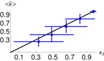
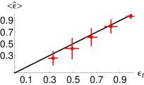
Figure 3: (Color online) Estimated value of entanglement as a function of the reference one assuming, for the description of the output signals, the families $\varrho$ (left plot) and $\varrho^{\prime}$ (right plot). The uncertainty bars stays for the $3\sigma$ confidence interval.

Notice that the reference value is built, on the basis of a given model, in part with informations coming from the experimental settings (the tuning of the angle $\phi$) and in part from the results of suitably chosen coincidence measurements. On the other hand, the estimated value of entanglement is obtained solely with experimental quantities. In principle, we are not expecting the reference value to be more precise that the estimated one. The idea here is to use two different estimates of the same quantity (entanglement) obtained in two different and independent ways in order to to discriminate and validate the different statistical models. Following our analysis, a given model is not suitable for the description of our system if the two different estimates that can be derived by that model, together with the resulting errors, are not compatible.

It is interesting to compare these results, in particular the ones which refer to the decoherence model (left plot in Fig. 3), with those obtained for a different set of measurements data presented in EEE . In that case a less precise control of the temperature of the PDC generation system made more relevant the fluctuation of the phase and thus the state more mixed. Therefore, in that case, a self-consistent statistical analysis of the acquired data allowed discriminating between the two statistical models identifying the decoherence model of Eq. (10) as the correct one for the experimental set up used in EEE . In the present case, which includes that the already mentioned control in temperature, the states obtained are nearly pure and thus one cannot expect the different characterization of noise to be relevant. Furthermore, to experimentally obtain more pure state one should reduce the collection angle of PDC emission. This obviously reduces the rate of coincidence counts, thus inducing an increase of the variance of both the estimators, for negativity and purity parameter respectively.

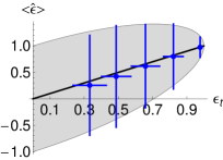
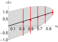
Figure 4: (Color Online) Estimation of entanglement at the quantum limit. The plot shows the estimated value of entanglement $\langle\hat{\epsilon}\rangle$ according to the decoherence (left) and Werner (right) models as a function of the reference one $\epsilon_{t}$. The uncertainty bars on $\langle\hat{\epsilon}\rangle$ denotes the quantity $\sqrt{\hbox{Var}(\hat{\epsilon})\times\langle K\rangle}$, i.e. the square root of the sample variance multiplied by the average number of total coincidences $\langle K\rangle$. The gray area corresponds to values within the inverse of the quantum Fisher information $\epsilon_{t}\pm H_{\epsilon_{t}}^{-1/2}$. Uncertainty bars on the abscissae are due to fluctuations in the estimation of the mixing parameter.

We now pass to evaluate the optimality of our estimation procedure. In Fig. 4 we show, for the decoherence (left) and Werner (right) model, the estimated value of entanglement as a function of the reference one obtained for different values $q=0.97,0.93,0.88,0.78,0.5$ (i.e. $\phi=10^{\circ},15^{\circ},20^{\circ},28^{\circ},45^{\circ}$). Note that the corresponding estimated mixing parameter in both model is larger than $0.97$ for all points. The uncertainty bars on $\langle\hat{\epsilon}\rangle$ denotes the quantity $\sqrt{\hbox{Var}(\hat{\epsilon})\times\langle K\rangle}$, i.e. the square root of the sample variance multiplied by the average number of total coincidences $\langle K\rangle$. This is in order to allow a direct comparison with the Cramer-Rao bound in term of the inverse of the Fisher information (the gray area). Uncertainty bars on the abscissae correspond to fluctuations $\delta\epsilon_{t}$ in the determination of $\epsilon_{t}$, due to fluctuations in the estimation of the mixing parameter with the procedure outlined above. The plot shows that our procedure allows estimating the entanglement with a precision at the quantum limit for any value of $q$. From the figure it is also apparent that, due to the high purity achieved with the experimental set up that includes the active temperature control, and, therefore, due to the irrelevance of the decoherence introduced, both the models give optimal estimation. Notice that this conclusion is robust against the fact that the statistics is not exactly Poissonian.

VI.2 Comparison with tomographic estimation

We compared our results with estimation of entanglement from density matrix elements obtained exploiting two different procedures of quantum state tomography KB00 ; Ja01 . We found that the reconstructed density matrices are, for both tomography protocols, statistically compatible within with both the two models of Eqs. (10) and (21). As an example we present in Fig. 5 real and imaginary part of reconstructed density matrices of maximally entangled state corresponding to $q=\frac{1}{2}$ (i.e., $\phi=45^{\circ}$).

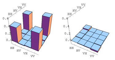
Figure 5: (Color online) Real (left) and Imaginary (right) part of the tomographically reconstructed density matrix for the maximally entangled state with J16 (top) and R16 (bottom) protocols. All the real elements, except the four dominant, and the imaginary ones are compatible with zero within the estimated tomographic uncertainties (not shown in the figure).

In fact, the tomographic procedure also allowed us to estimate entanglement and the corresponding variance. In order to have a fair comparison of the uncertainties obtained with different methods we have set measurement time for the tomographic reconstruction such to have thr total number of registered coincidences counts equal to $M\langle K\rangle$, i.e. the total number of coincidence in the optimal measurement. The values of negativity calculated directly using the reconstructed density matrices and its variance (obtained by error propagation) for the maximally entangled state are presented in Table 1 together with the determination obtained from the optimal measurement maximizing the QFI. All three negativity values overlap in their uncertainty intervals; the three methods are therefore coherent. Furthermore, it is evident from the presented results that the optimal method devised in this paper allows, at fixed sample size, for a sensitive reduction of the uncertainty in entanglement estimation.

Method	$\epsilon$		$\delta\epsilon$
Optimal	0.972	$\pm$	0.011
Tomography: J16	0.984	$\pm$	0.048
Tomography: R16	0.957	$\pm$	0.046

Table 1: Estimated value of entanglement with different methods. The uncertainty $\delta\epsilon$ is calculated usinv Eq. (28) for the optimal method and with error propagation for tomographic estimation.

VI.3 Statistical mixtures

In order to check our method in different working regimes we applied the estimation procedure to a set of mixed states obtained in a controlled way, i.e. by adding some portion of unentangled light to pure entangled state. As we have described in the previous section, our experimental set up allows us to obtain states with an extremely high purity. In the following we thus assume that the output state of our apparatus is the pure state as in Eq. (11). Then, if one is able, for example, to mix in a controlled way the components $\left|HH\rangle\!\langle HH\right|$ and $\left|VV\rangle\!\langle VV\right|$ to the maximally entangled states one obtains the states

$$\varrho = p\left|\psi\rangle\!\langle\psi\right|+(1-p)\,D$$ (29)

$$D = \frac{1}{2}\left(\left|HH\rangle\!\langle HH\right|+\left|VV\rangle\!\langle VV\right|)\right)\,,$$

which correspond to the model (10) with an adjustable mixing parameter. In practice, in order to tune the value of the mixing parameter $p$ we have measured coincidence counts for states $\left|{\hbox{\small HH}}\rangle\!\langle{\hbox{\small HH}}\right|$ and $\left|{\hbox{\small VV}}\rangle\!\langle{\hbox{\small VV}}\right|$ for different time intervals. The sample of coincidence counts is then added to experimental data obtained for the maximally entangled pure state and then analyzed as in the previous section.

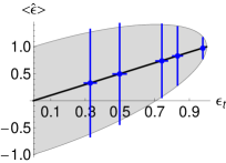
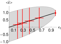
Figure 6: (Color Online) Estimation of entanglement at the quantum limit. The plot shows the estimated value of entanglement $\langle\hat{\epsilon}\rangle$ as a function of the reference one $\epsilon_{t}$. In the left panel we report estimated entanglement for mixed states generated according to the decoherence model (29). In the right panel we report estimated entanglemed for mixed states generated according to the Werner model (30). The points correspond to different portions of incoherent addition from both crystals.

In the left panel of Fig. 6 we show the estimated value of entanglement as a function of the reference one for the originally maximally entangled state ($q=\frac{1}{2}$) and for states prepared with mixing parameter $p=99.5\%,83\%,74\%,50\%,33\%$.

A similar analysis may carried out for the Werner model. In this case, in order to tune the value of the mixing parameter $p$ one should supplement the coincidences vectors $\bf{k}_{j}$ and $\bf{r}_{j}$ with values coming from unpolarized light. This can be achieved by measuring coincidence counts for $\left|{\hbox{\small HH}}\rangle\!\langle{\hbox{\small HH}}\right|$, $\left|{\hbox{\small HV}}\rangle\!\langle{\hbox{\small HV}}\right|$, $\left|{\hbox{\small VH}}\rangle\!\langle{\hbox{\small VH}}\right|$ and $\left|{\hbox{\small VV}}\rangle\!\langle{\hbox{\small VV}}\right|$ for different time intervals. The measured values are then added to the previously measured values for pure maximally entangled state. In this way, one can get data corresponding to

$$\varrho^{\prime}=p\left|\psi\rangle\!\langle\psi\right|+(1-p)\frac{\mathbbm{I}}{4}$$ (30)

which correspond to a Werner state with tunable depolarizing parameter. After performing measurement and analysis set described in previous section we can estimate entanglement and mixing parameter value in this family of states. In the right panel Fig. 6 we show the estimated value of entanglement as a function of the actual one for the originally maximally entangled state and mixture parameter $p=99.5\%,76\%,62\%,52\%,45\%$. As one can evince from the presented figure our method provides optimal entanglement estimation also for mixed states.

VII Conclusions

In this paper we have addressed in detail the estimation of entanglement for pairs of polarization qubits. Our scheme is based on visibility measurements of quantum correlations and allows optimally estimating entanglement of families of two-photon polarization entangled states without the need of performing full tomography. Our procedure is self-consistent and allows estimating the amount of entanglement with the ultimate precision imposed by quantum mechanics. Although optimal estimation of entanglement does not require the full tomography of the states we have also performed state reconstruction using two different sets of projectors and explicitly shown that they provide a less precise determination of entanglement.

The technique has been demonstrated for nearly pure states as well as for controlled mixtures in order to confirm its reliability in any working regime. With a suitable choice of correlation measurements it may be extended to a generic class of two-photon entangled states. The statistical reliability of our method suggests a wider use in precise monitoring of external parameters assisted by entanglement.

References

- (1) R. Horodecki, P. Horodecki, M. Horodecki, and K. Horodecki, Rev. Mod. Phys. 81, 865 (2009).
- (2) O. Gühne and G. Toth, Phys. Rep. 474, 1 (2009).
- (3) R. Augusiak and M. Lewenstein, Q. Inf. Proc. 8, 493 (2009).
- (4) P. Lougovski and S. J. Van Enk, Phys. Rev. A 80, 052324 (2009); Phys. Rev. A 80, 034302 (2009).
- (5) H. Wunderlich and M. B. Plenio, J. Mod. Opt. 56, 2100 (2009).
- (6) J. Eisert, F. G. S. L. Brandao, and K. M. Adenauert, New J. Phys. 9, 46 (2007).
- (7) K. Audenaert and M. B. Plenio, New J. Phys. 8, 266 (2006).
- (8) M. G. A. Paris and J. Rehacek (Eds.), Lect. Not. Phys. 649, (Springer, Berlin, 2004).
- (9) G. M. D’Ariano, C. Macchiavello, and M. G. A. Paris, Phys. Lett. A 195, 31 (1994).
- (10) M. Asorey, P. Facchi, G. Florio, V. I. Man’ko, G. Marmo, S. Pascazio, and E. C. G. Sudarshan, Phys. Lett. A 375, 861 (2011).
- (11) G. Jaeger, M. A. Horne, and A. Shimony, Phys. Rev. A 48, 1023 (1993).
- (12) J. F. Clauser, M. A. Horne, A. Shimony, and R. Holt, Phys. Rev. Lett. 23, 880 (1969).
- (13) R. F. Werner and M. Wolf, Quant. Inf. Comp. 1, 1 (2001).
- (14) M. Horodecki, P. Horodecki, and R. Horodecki, Phys. Lett. A 223, 1 (1996).
- (15) B. M. Terhal, Phys. Lett. A 271, 319 (2000).
- (16) O. Gühne, P. Hyllus, D. Bruß, A. Ekert, M. Lewenstein, C. Macchiavello, and A. Sanpera, Phys. Rev. A 66, 062305 (2002).
- (17) F. G. S. L. Brandao and R. O. Vianna, Int. Journ. Quant. Inf. 4 331 (2006).
- (18) P. Krammer, H. Kampermann, D. Bruß, R. A. Bertlmann, L. C. Kwek, and C. Macchiavello, Phys. Rev. Lett. 103, 100502 (2009).
- (19) P. Facchi, G. Florio, and S. Pascazio, Int. Journ. Q. Inf. 5, 97 (2007).
- (20) M. V. Fedorov, M. A. Efremov, P. A. Volkov, and J. H. Eberly, J. Phys. B: At. Mol. Opt. Phys., 39, 467 (2006).
- (21) P. A. Volkov, Y. M. Mikhailova, and M. V. Fedorov, Adv. Science. Lett. 2, 511 (2009).
- (22) M. Genovese, Phys. Rep. 413, 319 (2005).
- (23) M. Bourennane, M. Eibl, C. Kurtsiefer, S. Gaertner, H. Weinfurter, O. Gühne, P. Hyllus, D. Bruß, M. Lewenstein, and A. Sanpera, Phys. Rev. Lett. 92, 087902 (2004).
- (24) M. V. Fedorov, M. A. Efremov, P. A. Volkov, E. V. Moreva, S. S. Straupe, and S. P. Kulik, Phys. Rev. Lett 99, 063901 (2007); Phys. Rev. A 77, 032336 (2008).
- (25) G. Brida, V. Caricato, M. V. Fedorov, M. Genovese, M. Gramegna, and S. P. Kulik, Europhys. Lett. 87, 64003 (2009).
- (26) M. Avenhaus, M. V. Chekhova, L. A. Krivitsky, G. Leuchs, and C. Silberhorn, Phys. Rev. A 79, 043836 (2009).
- (27) M. Barbieri, F. De Martini, G. Di Nepi, P. Mataloni, G. M. D’Ariano, and C. Macchiavello, Phys. Rev. Lett. 91, 227901 (2003).
- (28) S. P. Walborn, P. H. Souto Ribeiro, L. Davidovich, F. Mintert, and A. Buchleitner, Nature 440, 1022 (2006).
- (29) M. P. Almeida, F. de Melo, M. Hor-Meyll, A. Salles, S. P. Walborn, P. H. Souto Ribeiro, and L. Davidovich, Science 316, 579 (2007).
- (30) M. G. Genoni, P. Giorda, and M. G. A. Paris Phys. Rev. A 78, 032303 (2008).
- (31) C. W. Helstrom, Phys. Lett. A 25, 1012 (1967); C. W. Helstrom, Quantum detection and estimation theory, (Academic Press, New York, 1976).
- (32) S. L. Braunstein and C. M. Caves, Phys. Rev. Lett. 72, 3439 (1994); S. L. Braunstein, C. M. Caves, and G. J. Milburn, Ann. Phys. 247, 135 (1996).
- (33) D. C. Brody and L. P. Hughston, Proc. Roy. Soc. Lond. A 454, 2445 (1998); 455, 1683 (1999).
- (34) M. G. A. Paris, Int. J. Q. Inf. 7, 125 (2009).
- (35) G. Brida, I. P. Degiovanni, A. Florio, M. Genovese, P. Giorda, A. Meda, M. G. A. Paris, and A. Shurupov, Phys. Rev. Lett. 104, 100501 (2010).
- (36) P. G. Kwiat, E. Waks, A. G. White, I. Appelbaum, and P. H. Eberhard, Phys. Rev. A 60, R733 (1999).
- (37) M. Genovese, G. Brida, C. Novero, and E. Predazzi, Phys. Lett. A 268 12 (2000).
- (38) Yu. I. Bogdanov, E. V. Moreva, G. A. Maslennikov, R. F. Galeev, S. S. Straupe, and S. P. Kulik, Phys. Rev. A 73, 063810 (2006).
- (39) K. Banaszek, G. M. D’Ariano, M. G. A. Paris, and M. F. Sacchi, Phys. Rev. A 61, 10304 (2000).
- (40) D. F. V. James, P. G. Kwiat, W. J. Munro and A. G. White, Phys. Rev. A, 64, 052312 (2001).
- (41) Yu. I. Bogdanov, M. V. Chekhova, L. A. Krivitsky, S. P. Kulik, A. N. Penin, A. A. Zhukov, L. C. Kwek, C. H. Oh, and M. K. Tey, Phys. Rev. A, 70, 042303 (2004).
- (42) J. Rehácek, B. Englert, and D. Kaszlikowski, Phys. Rev. A 70, 052321 (2004).
- (43) M. D. de Burgh, N. K. Langford, A. C. Doherty, and A. Gilchrist, Phys. Rev. A 78, 052122 (2008).
- (44) Yu. I. Bogdanov, G. Brida, M. Genovese, S. P. Kulik, E. V. Moreva, A. P. Shurupov, Phys. Rev. Lett. 105, 010404 (2010).