Numerical Modeling of Radiation-Dominated and QED-Strong Regimes of Laser-Plasma Interaction

Abstract

Ultra-strong laser pulses can be so intense that an electron in the focused beam loses significant energy due to $\gamma$-photon emission while its motion deviates via the radiation back-reaction. Numerical methods and tools designed to simulate radiation-dominated and QED-strong laser-plasma interactions are summarized here.

I Introduction

Progress in laser technologies has resulted in the opportunity to create ultra-strong electromagnetic fields in tightly focused laser beams. In the present paper we discuss the numerical methods designed to simulate processes in strong pulsed laser fields interacting with plasma. Attention is paid to the recently achieved range of intensities, $J\geq 2\cdot 10^{22}{\rm W/cm}^{2}$ 1022 , and the larger intensities projected, $J\sim 10^{25}{\rm W/cm}^{2}$ ELI .

For a typical laser wavelength, $\lambda\sim 1\mu$m, electron motion in laser fields at $J\geq 10^{18}{\rm W/cm}^{2}$ is relativistic:

$$|{\bf a}|\gg 1,\qquad{\bf a}=\frac{e{\bf A}}{m_{e}c^{2}},$$ (1)

where $m_{e}$ and $e=-|e|$ are the mass and the electric charge of electron.

However, if we want to evaluate the properties of an electron in a strong field as an emitting particle, moreover, a particle, which emits photons we need to be guided by the more severe condition:

$$|{\bf a}|_{\alpha}=\alpha|{\bf a}|\geq 1,$$ (2)

in which the fundamental fine structure constant is present, $\alpha=e^{2}/(c\hbar)\approx 1/137$, linking its radiation to its motion (herewith, the subscript $\alpha$ denotes the dimensionless parameter multiplied by $\alpha$). With the recently achieved intensity of $J\sim 2\cdot 10^{22}\ {\rm W/cm}^{2}\sim(1/\alpha^{2})\cdot 10^{18}\ {\rm W/cm^{2}}$, this newly important dimensionless parameter exceeded unity!

However, this estimate could be applicable only to a ’theoretical laser’, for which the photon energy, $\hbar\omega$, would be comparable to the ’characteristic’ atomic unit of energy, ${\rm 2Ry}=\alpha^{2}m_{e}c^{2}$. For a real laser, in addition to the field magnitude, importance rests on the laser photon energy normalized by ${\rm 2Ry}$:

$$\omega_{\rm 2Ry}=\frac{\hbar\omega}{\rm 2Ry}\approx\frac{45{\rm nm}}{\lambda},\qquad{\rm 2Ry}=\alpha^{2}m_{e}c^{2}\approx 27.3{\rm eV}.$$ (3)

For the majority of ultra-strong lasers this parameter is of the order of $10^{-1}$: $\omega_{\rm 2Ry}\sim 0.04$ for the Nd-glass laser ($\lambda\approx 1.06\ \mu$m), $\omega_{\rm 2Ry}\sim 0.06$ for the Ti-sapphire laser ($\lambda\approx 0.8\ \mu$m). Therefore, the following product,

$$\omega_{\rm 2Ry}\left|\frac{d{\bf a}}{d\xi}\right|_{\alpha}=\sqrt{\frac{J}{J_{p}}},\quad J_{p}=\frac{cE_{p}^{2}}{4\pi}\approx 2.4\cdot 10^{25}{\rm W/cm}^{2},$$ (4)

is less than one even for planned intensities (although $|d{\bf a}/d\xi|_{\alpha}$ might be greater than one). Herewith, the estimates are made for the 1D wave field, ${\bf a}={\bf a}(\xi)$, $\xi=\omega(t-x/c)$, $0\leq\xi\leq\xi_{\rm max}$. Eq.(4) is expressed in terms of the local instantaneous intensity of the laser wave, $J$. Note that the Left Hand Side (LHS) of Eq.(4) equals the ratio, $|{\bf E}|/E_{p}$, of the wave electric field, $|{\bf E}|=\sqrt{4\pi J/c}$, to the characteristic field, $E_{p}=|e|/\lambdabar_{C}^{2}$, constructed from an elementary charge and the Compton wavelength:

$$\lambdabar_{C}=\frac{\hbar}{m_{e}c}\approx 3.9\cdot 10^{-11}{\rm cm},\quad\lambda_{C}=2\pi\lambdabar_{C}\approx 2.4\cdot 10^{-10}{\rm cm}.$$

This field strength is associated with the Coulomb field between the components of a virtual electron-positron pair (which are ’separated’ by the Compton wavelength). Across the interval of intensities bounded by Ineq.(2) from below and by Eq.(4) from above, that is, at

$$\omega_{\rm 2Ry}\approx\frac{45{\rm nm}}{\lambda}\leq\sqrt{\frac{J}{J_{p}}}\leq 1$$ (5)

the role of important physical effects changes dramatically, incorporating radiation and its back-reaction, and QED effects of electron recoil and spin as well as pair production. Given that currently available laser intensities can access this kind of interaction, it is clear that the development of a suitable model is timely.

Radiation-dominated laser fields. An accelerated electron in a strong laser field emits high-frequency radiation. The radiation back-reaction decelerates such an electron, the effect being more pronounced for longer laser pulses our . In Ref.kogaetal a condition for the field to be radiation-dominated is formulated in terms of the ratio between the magnitudes of the Lorentz force and of the radiation force, which gives:

$$\frac{2}{3}\omega_{\rm 2Ry}({\cal E}-p_{\|})_{\alpha}\left(\left|\frac{d{\bf a}}{d\xi}\right|_{\alpha}\right)^{2}\geq 1.$$ (6)

Herewith the electron dimensionless energy, ${\cal E}$, and its momentum, ${\bf p}$, are related to $m_{e}c^{2}$, and $m_{e}c$ correspondingly, and subscript $\|$ herewith denotes the vector projection on the direction of the wave propagation.

While a strong laser pulse interacts with energetic electrons, which move oppositely to the direction of the pulse propagation, the condition ${\cal E}-p_{\|}\approx 2{\cal E}\gg 1$, facilitates the fulfillment of Ineq.(6). In the course of a strong laser pulse interacting with a dense plasma the counterpropagating electrons may be accelerated in a backward direction by a charge separation field. For this reason, the radiation effects in the course of laser-plasma interaction are widely investigated (see Refs.kogaetal ; lau03 ; FI ) and efficient computational tools are in demand.

QED-strong laser fields. In Quantum Electro-Dynamics (QED) an electric field should be treated as strong if it exceeds the Schwinger limit: $|{\bf E}|\geq E_{S}=m_{e}c^{2}/(|e|\lambdabar_{C})$ (see Ref.schw ). Such field is potentially capable of separating a virtual electron-positron pair providing an energy, which exceeds the electron rest mass energy, $m_{e}c^{2}$, to a charge, $e=\mp|e|$, over an acceleration length as small as the Compton wavelength. Typical effects in QED-strong fields are high-energy photon emission from electrons or positrons and electron-positron pair creation from high-energy photons (see Refs.Mark ; kb ; ourPRL ).

Here we assume that the field invariants (see ll ) are small as compared to the Schwinger field:

$$|E^{2}-B^{2}|\ll E_{S}^{2},\qquad|({\bf E}\cdot{\bf B})|\ll E_{S}^{2},$$ (7)

${\bf B}$ being the magnetic field. Below, the term “QED-strong field” is only applied to the field experienced by a particle. For example, a particle in the 1D wave field, may experience a QED-strong field, $E_{0}=|d{\bf A}/d\xi|\omega({\cal E}-p_{\|})/c$, because the laser frequency is Doppler upshifted in the comoving frame of reference. The Lorentz-transformed field exceeds the Schwinger limit, if

$$\chi=\frac{2}{3}E_{0}/E_{S}=\frac{2\lambdabar_{C}}{3\lambdabar}({\cal E}-p_{\|})\left|\frac{d{\bf a}}{d\xi}\right|\gg 1,$$ (8)

where $\lambdabar=c/\omega$. Numerically, the parameter, $\chi$, equals:

$$\chi=\frac{3}{2}\omega_{\rm 2Ry}({\cal E}-p_{\|})_{\alpha}\left|\frac{d{\bf a}}{d\xi}\right|_{\alpha}\approx 0.7\frac{({\cal E}-p_{\|})}{10^{3}}\sqrt{\frac{J}{10^{23}[{\rm W/cm}^{2}]}}.$$

Estimates for laser-driven electrons. In the critical parameters as in Ineqs.(6,8) the factor, ${\cal E}-p_{\|}$ is not linked to the wave intensity in the case where electrons are accelerated by an external source. In the course of the laser-plasma interaction, however, for bulk electrons $({\cal E}-p_{\|})\sim{\cal E}\sim|{\bf p}_{\perp}|$. As long as the radiation back-reaction does not dominate, the conservation law for the generalized momentum of electron gives: ${\bf p}_{\perp}\approx-{\bf a}$, and the LHS of Eqs.(6) may be evaluated in terms of the vector potential amplitude, $a_{0}$. The wave becomes radiation-dominated (see Ineq.6), if:

$$a_{0}\geq(\omega_{\rm 2Ry})^{-1/3},\quad J\geq J_{p}(\omega_{\rm 2Ry})^{4/3}\sim(3-5)\cdot 10^{23}{\rm W/cm}^{2}.$$

Less certain is the estimate for the significance of QED effects. On one hand, for fields just approaching the radiation-dominated regime QED effects are already not fairly neglected: $\chi\sim(3/2)(\omega_{\rm 2Ry})^{1/3}\approx(0.5-0.6)$. On the other hand, in radiation-dominated fields the estimate for ${\cal E}$ that we used above is not reliable. Because of this complexity, we surmise that the significance of QED effects in this regime can only be verified by direct numerical simulations.

Paper content and structure. Numerical simulations of laser-plasma interactions become increasingly complicated while proceeding to higher intensities. At intensities $J\geq 2\cdot 10^{22}{\rm W/cm}^{2}$ the model should incorporate the radiation back-reaction on the emitting electron. In this range $\chi\ll 1$ for bulk electrons, making the QED-effects negligible. This model is presented in Sec. II. At $J\geq 3\cdot 10^{23}{\rm W/cm}^{2}$ the QED corrrections should be incorporated to achieve a quantitative accuracy for electrons with $\chi\sim 1$. These corrections may be found in Sec. III. At larger intensities, $J\geq 10^{24}{\rm W/cm}^{2}$ the high-energy photons emitted by electrons and positrons produce a macroscopically large number of electron-positron pairs, as shown in Sec. IV.

In each section we first summarize the theoretical model. Then we provide the analytical solutions, which may be used to benchmark numerical models. After this we describe the elements of the numerical scheme.

II QED-weak fields ($\chi\ll 1$)

II.1 Theoretical notes

II.1.1 Emission spectrum

In Ref.jack the spectral and angular distribution, $d{\cal E}_{\rm rad}/(d\omega^{\prime}d{\bf n})$, of the radiation energy, emitted by an electron and related to the interval of frequency, $d\omega^{\prime}$, and to the element of solid angle, $d{\bf n}$, for a polarization vector, ${\bf l}$, is described with the following formula:

$$\frac{d{\cal E}_{\rm rad}(\omega^{\prime},{\bf n},{\bf l})}{d\omega^{\prime}d{\bf n}}=\frac{(\omega^{\prime})^{2}}{4\pi^{2}c}\left|({\bf A}_{\rm cl}(\omega^{\prime})\cdot{\bf l}^{*})\right|^{2}.$$ (9)

Here the vector amplitude of emission, ${\bf A}_{\rm cl}(\omega^{\prime})$, is given by the following equation:

$${\bf A}_{\rm cl}(\omega^{\prime},{\bf n})=\frac{e}{c}\int_{-\infty}^{+\infty}{{\bf v}(t)\exp\left(i\omega^{\prime}\left\{t-\frac{[{\bf n}\cdot{\bf x}(t)]}{c}\right\}\right)dt},$$

see Eq.(14.67) in Ref.jack . We express $d{\cal E}_{\rm rad}/(d\omega^{\prime}d{\bf n})$ in terms of the time integral of the radiation loss rate, $dI_{\rm cl}/(d\omega^{\prime}d{\bf n})$, which is related to the unit of time, the element of a solid angle, and the frequency interval, and is summed over polarizations:

$$\frac{\partial}{\partial t}\left[\sum_{\bf l}{\frac{d{\cal E}_{\rm rad}}{d\omega^{\prime}d{\bf n}}}\right]=\frac{dI_{\rm cl}(t)}{d\omega^{\prime}d{\bf n}}.$$

The spectral and angular distribution of the radiation loss rate is given by the Fourier integral:

$$\frac{dI_{\rm cl}(\tau)}{d\omega^{\prime}d{\bf n}}=-\frac{e^{2}(\omega^{\prime})^{2}}{4\pi^{2}c{\cal E}(\tau)}\int_{-\infty}^{+\infty}\left[p\left(\tau+\frac{\zeta}{2}\right)\cdot p\left(\tau-\frac{\zeta}{2}\right)\right]\times$$

$$\times\exp\left\{ic\int_{\tau-\zeta/2}^{\tau+\zeta/2}{[k^{\prime}\cdot p(\tau^{\prime})]d\tau^{\prime}}\right\}d\zeta.$$

The cogent feature of the particle relativistic motion in strong laser fields is that the emitted radiation is abruptly beamed about the direction of the velocity vector, ${\bf p}(\tau)/|{\bf p}(\tau)|$. Therefore, the angular spectrum of emission can be approximated with the Dirac function:

$$\frac{dI_{\rm cl}(\tau)}{d\omega^{\prime}d{\bf n}}=\delta^{2}\left({\bf n}-\frac{\bf p}{|{\bf p}|}\right)\frac{dI_{\rm cl}(\tau)}{d\omega^{\prime}}.$$

In the frequency spectrum of emission,

$$\frac{dI_{\rm cl}(\tau)}{d\omega^{\prime}}=\frac{e^{2}\omega^{\prime}}{2\pi c{\cal E}^{2}(\tau)}\int_{-\infty}^{+\infty}\frac{1}{\zeta}\left[p\left(\tau+\frac{\zeta}{2}\right)\cdot p\left(\tau-\frac{\zeta}{2}\right)\right]\times$$

$$\times\sin\left[\frac{\omega^{\prime}}{{\cal E}(\tau)}\left(\frac{\zeta}{2}+\int_{\tau-\zeta/2}^{\tau+\zeta/2}\left\{[p(\tau)\cdot p(\tau^{\prime})]-1\right\}d\tau^{\prime}\right)\right]d\zeta,$$

for relativistically strong wave field, satisfying Eq.(1), the sine function oscillates fast, so that the main contribution to the integral determining the emission spectrum comes from a brief time interval with small values of $\zeta$, resulting in a universal emission spectrum:

$$\frac{dI_{\rm cl}(\tau)}{d\omega^{\prime}}=I_{\rm cl}\frac{Q_{\rm cl}(r)}{\omega_{c}},\qquad I_{\rm cl}=-\frac{2e^{2}(f_{Le}\cdot f_{Le})}{3m_{e}^{2}c^{3}},$$ (10)

$$Q_{\rm cl}(r)=\frac{9\sqrt{3}}{8\pi}r\int_{r}^{\infty}{K_{5/3}(r^{\prime})dr^{\prime}},\qquad r=\frac{\omega^{\prime}}{\omega_{c}},$$ (11)

$$\omega_{c}={\cal E}\chi.$$ (12)

Here $Q_{\rm cl}(r)$ is the unity-normalized spectrum of the gyrosynchrotron emission, such that $\int{Q_{\rm cl}(r)dr}=1$ and $K_{\nu}(r)$ are MacDonald functions. We use the dimensionless photon frequency, $\tilde{\omega}^{\prime}=\hbar\omega^{\prime}/(m_{e}c^{2})$, the characteristic frequency, $\tilde{\omega}_{c}=\hbar\omega_{c}/(m_{e}c^{2})$, and the dimensionless wave vector, $\tilde{\bf k}^{\prime}=\hbar{\bf k}^{\prime}$, for emitted $\gamma$-photons and omit tildes in the formulae. Both the radiation energy loss rate, $I_{\rm cl}$, and the QED-strength parameter,

$$\chi=\frac{3}{2}\frac{\lambdabar_{C}\sqrt{-(f_{Le}\cdot f_{Le})}}{m_{e}c^{2}},$$ (13)

are expressed in terms of the 4-square of the Lorentz 4-force: $f^{\mu}_{Le}={\cal E}({\bf f}_{Le}\cdot{\bf u}/c,{\bf f}_{Le})$, where ${\bf u}=c{\bf p}/\sqrt{1+{\bf p}^{2}}$ is the velocity and ${\bf f}_{Le}=e{\bf E}+\frac{e}{c}[{\bf u}\times{\bf B}]$ is the Lorentz three-force.

Thus, the acceleration of electrons by the laser pulse must be accompanied by gyrosynchrotron-like emission spectrum (which is actually observed - see Refs.Rousse ; kneip ). The general character of such emission spectrum had been noted in Ref.Rousse (this comment may be also found in Sec. 77 in Ref.ll ). The material of the present subsection was published in Ref.PRE .

II.1.2 Equation for the radiation emission and transport

The above considerations justify the method for calculating the high frequency emission as described in Ref.our (see also Rousse ). In addition to calculating the electromagnetic fields on the grid using a Particle-In-Cell (PIC) scheme, one can also account for the higher-frequency (subgrid) emission, by calculating its instantaneously radiated spectrum. Compared with direct calculation of the RHS of Eq.(9) (the means of calculating the emission used, for example, in Ref.spie ,t0 ) the approach suggested here, though mathematically equivalent, may be decidedly more efficient.

Generally, the Radiation Transport Equation (RTE, cf. Ref.ZR ) should be solved for the radiation energy density, related to the element of volume, $dV$ (herewith the symbol $\sum_{\bf l}$ is omitted):

$${\cal I}=\frac{d{\cal E}_{\rm rad}}{d\omega^{\prime}d{\bf n}dV}.$$

An electron located at the point, ${\bf x}={\bf x}_{e}(t)$, contributes to the right hand side (RHS) of the RTE as follows:

$$\frac{\partial{\cal I}}{\partial t}+c({\bf n}\cdot\nabla){\cal I}=\sum_{e}{\frac{I_{\rm cl}Q_{\rm cl}(r)}{\omega_{c}}\delta^{2}\left({\bf n}-\frac{\bf p}{p}\right)\delta^{3}({\bf x}-{\bf x}_{e})}.$$

The LHS of the RTE describes the radiation transport, while in the RHS, in addition to the emission source, there should be the terms accounting for the radiation absorption and scattering. However, at $\chi\ll 1$ and at realistic plasma densities these effects may be neglected. Under these circumstances the RTE can be easily integrated over time and space, giving:

$$\frac{d{\cal E}_{\rm rad}}{d\omega^{\prime}d{\bf n}}=\int_{0}^{t}{\left(\sum_{e}{\frac{I_{\rm cl}Q_{\rm cl}(r)}{\omega_{c}}\delta^{2}({\bf n}-\frac{\bf p}{p})}\right)dt}$$ (14)

Since Eq.(14) depends on frequency only via $Q_{\rm cl}(r)$, one can calculate instead of Eq.(14) an integral as follows

$$\frac{d{\cal E}^{(m)}_{\rm rad}}{d{\bf n}d\bar{\omega}}=\int_{0}^{t}{\left[\sum_{e}{\frac{I_{\rm cl}}{\omega_{c}}\delta^{2}\left({\bf n}-\frac{{\bf p}}{p}\right)\delta\left(\log\bar{\omega}-\log\omega_{c}\right)}\right]dt}.$$

Once this modified spectrum has been integrated over the whole simulation time, a true spectral distribution can be recovered using a simple convolution as follows:

$$\frac{d{\cal E}_{\rm rad}(\omega^{\prime},{\bf n})}{d{\bf n}d\omega^{\prime}}=\int{Q_{\rm cl}\left(\frac{\omega^{\prime}}{\bar{\omega}}\right)\frac{d{\cal E}^{(m)}_{\rm rad}(\bar{\omega},{\bf n})}{d{\bf n}d\bar{\omega}}d\log\bar{\omega}}.$$ (15)

Manifestly, the result is the same, which allows one to avoid calculating the spectrum, $Q_{\rm cl}(r)$, at each time step.

II.1.3 Equation for electron motion: accounting the radiation back-reaction

Here we use the equation of motion for a radiating electron as derived in Refs.our ; mine . In 4-vector form this equation may be written for the electron 4-momentum, $p^{\alpha}$, normalized per $m_{e}c$, in terms of the Lorentz 4-force, $f^{\alpha}_{Le}=eF^{\alpha\beta}p_{\beta}$ and the field 4-tensor, $F^{\alpha\beta}=({\bf E},{\bf B})$:

$$\frac{dp^{\alpha}}{d\tau}=\frac{e}{m_{e}c^{2}}F^{\alpha\beta}\frac{dx_{\beta}}{d\tau}-\frac{I_{\rm cl}p^{\alpha}}{mc^{2}},$$ (16)

$$\frac{dx^{\alpha}}{d\tau}=cp^{\alpha}+\frac{\tau_{0}f^{\alpha}_{Le}}{m_{e}},\qquad\tau_{0}=\frac{2e^{2}}{3m_{e}c^{3}}.$$ (17)

Three-vector formulation of Eqs.(16-17) is:

$$\frac{d{\bf p}}{dt}=\frac{{\bf f}_{Le}}{m_{e}c}+\frac{e[\bar{\bf u}\times{\bf B}]}{m_{e}c^{2}}-\frac{{\bf u}{\cal E}^{2}(\bar{\bf u}\cdot{\bf f}_{Le})}{m_{e}c^{3}},$$ (18)

$$\frac{d{\bf x}}{dt}={\bf u}+\bar{\bf u},\quad\bar{\bf u}=\frac{\tau_{0}}{m_{e}}\frac{{\bf f}_{Le}-{\bf u}({\bf u}\cdot{\bf f}_{Le})/c^{2}}{1+\tau_{0}({\bf u}\cdot{\bf f}_{Le})/(mc^{2})}.$$

II.1.4 Comparison with the Landau-Lifshitz equation.

Many authors simulate motion of an emitting electron using the equation as suggested by Landau and Lifshitz (LL - see Eq.(76.3) in ll ), motivating a comparison with the approach we use. To simplify the formulae, we introduce the 4-velocity, $u^{i}$, and normalize the field tensor:

$$u^{\alpha}=\frac{1}{c}\frac{dx^{\alpha}}{d\tau},\qquad\tilde{F}^{\alpha\beta}=\frac{\tau_{0}eF^{ik}}{m_{e}c}=\frac{2\alpha F^{ik}}{3E_{S}}.$$

All 4-vector equations in this paragraph are written without indices and the tensor multiplication is denoted with dot-product and/or powers of tensor, e.g. $\tilde{F}\cdot u=\tilde{F}^{ik}u_{k}$, $\tilde{F}^{2}\cdot u=\tilde{F}\cdot\tilde{F}\cdot u=\tilde{F}^{ik}\tilde{F}_{kl}u^{l}$ etc. Now we re-write the LL equation:

$$\frac{du}{d\tau}=\frac{1}{\tau_{0}}\tilde{F}\cdot\left(u+\tilde{F}\cdot u\right)+\frac{d\tilde{F}}{d\tau}\cdot u-\frac{u}{\tau_{0}}(u\cdot\tilde{F}^{2}\cdot u).$$ (19)

and compare it with Eqs.(16,17):

$$\frac{dp}{d\tau}=\frac{1}{\tau_{0}}\tilde{F}u-\frac{p}{\tau_{0}}(p\cdot\tilde{F}^{2}\cdot p),\qquad u=p+\tilde{F}\cdot p.$$ (20)

Solving the momentum from the second of Eqs.(20), $p=\sum_{n=0}^{\infty}{(-\tilde{F})^{n}\cdot u}.$ Accounting for the anti-symmetry of the field tensor, the first of Eqs.(20) may be re-written for 4-velocity and 4-acceleration, similarly to Eq.(19):

$$\frac{du}{d\tau} = \frac{1}{\tau_{0}}\tilde{F}\cdot\left(u+\tilde{F}\cdot u\right)+$$ (21)

$$+ \frac{d\tilde{F}}{d\tau}\cdot\sum_{n=0}^{\infty}{(-\tilde{F})^{n}}\cdot u-\frac{u}{\tau_{0}}(u\cdot\sum_{n=1}^{\infty}{\tilde{F}^{2n}}\cdot u).$$

The only distinction from Eq.(19) is that in Eq.(21) the infinite series are present, while in Eq.(19) there are only starting terms of these series.

How large is the difference numerically? For the second series one may evaluate both the total sum:

$$u\cdot\sum_{n=1}^{\infty}{\tilde{F}^{2n}}\cdot u=p\cdot\tilde{F}^{2}\cdot p=\left(\frac{2}{3}\alpha\right)^{2}\left(\frac{4}{9}\chi^{2}\right),$$

and the residual sum, omitted in Eq.(19):

$$u\cdot\sum_{n=2}^{\infty}{\tilde{F}^{2n}}\cdot u=\left(\frac{2}{3}\alpha\right)^{4}\left(\frac{4}{9}\chi^{2}\frac{E^{2}-B^{2}}{E_{s}^{2}}+\frac{({\bf E}\cdot{\bf B})^{2}}{E_{s}^{4}}\right).$$

The residual sum is reduced by a factor, $(2\alpha/3)^{2}(E^{2}-B^{2})/E_{S}^{2}$, which is small according to Ineq.(7).

How theoretically important is the distinction between the two approaches? We discussed this issue in Refs.our ; mine and noted that the LL equation conserves neither the generalized momentum of electron nor the total energy-momentum of the system consisting of an emitting electron, the external field and the radiation. Another distinction is that the LL approach maintains the identity, $u^{2}=1$, while Eqs.(20) maintain more important identity, $p^{2}=1$, turning to the Dirac equation in the limit of QED-strong field. For the square of the 4-velocity we obtain:

$$u^{2}=p^{2}-p\cdot\tilde{F}^{2}\cdot p\approx 1-1.05\cdot 10^{-5}\chi^{2},$$ (22)

which is not exactly unity, but in QED-weak fields, $\chi\ll 1$, the distinction is negligible.

The computational advantage of Eqs.(20) as compared to the LL equation, is, first, the higher efficiency: compare the compact expression for three-force in Eq.(18) with that given in ll (see section 77, problem 2). Second, the numerical scheme for Eq.(18) is more reliable, as it is bound to yield total energy conservation. Thus, even for fields in the QED weak regime, the use of Eqs.(20) is more suitable than the use of the LL equation.

II.2 Analytical solution

Pertaining to the validation against a semi-analytical theory, we begin by describing the spectrum of emission from an electron in the field of a 1D circularly polarized wave. A constant wave amplitude, $a_{0}$ is assumed to be below the radiation-dominated regime. In this case ${\bf p}_{\perp}\approx-{\bf a}$, so that ${\cal E}^{2}-p_{\|}^{2}=1+a_{0}^{2}$. The modified spectrum can be expressed in terms of the characteristic frequency, which is a function of the current value of the electron energy:

$$\frac{\omega_{c}}{\omega_{c0}}=1+\frac{({\cal E}-p_{\|})^{2}}{1+a_{0}^{2}}\ ,$$ (23)

as well as the parameter, $\omega_{c0}$ which is introduced as the following function of the wave amplitude and frequency:

$$\omega_{c0}=\frac{3}{4}\omega_{\rm 2Ry}\alpha^{2}\left(a_{0}+a_{0}^{3}\right).$$ (24)

The maximum frequency of emission is determined by the initial momentum of electron:

$$\frac{\omega_{c{\rm max}}}{\omega_{c0}}=1+\frac{({\cal E}-p_{\|})^{2}_{\xi=0}}{1+a_{0}^{2}}\,.$$

Then, $\xi^{*}(\xi)$ is a normalized phase:

$$\xi^{*}=\left(\frac{2}{3}\alpha^{3}\omega_{\rm 2Ry}a_{0}^{2}\sqrt{1+a_{0}^{2}}\right)\xi,$$ (25)

For the whole pulse the total normalized phase,

$$\xi^{*}_{\infty}=\frac{2}{3}\alpha^{3}a_{0}^{2}\sqrt{1+a_{0}^{2}}\xi_{\rm max}\approx\frac{2}{3}\left(\frac{J}{J_{p}}\right)^{3/2}\frac{\xi_{\rm max}}{(\omega_{\rm 2Ry})^{2}},$$

characterizes the capability of the pulse to arrest the counterpropagating electron by means of the radiation back-reaction. Particularly, a pulse of duration corresponding to $\xi^{*}_{\infty}\geq 1$ arrests an electron of any energy. The modified spectrum has a shape close to a power-law (see derivation details in ourAIP ):

$$\frac{d{\cal E}^{(m)}_{\rm rad}}{d\bar{\omega}}=\frac{m_{e}c^{2}\sqrt{1+{\bf a}^{2}}}{4\omega_{c0}}\frac{\bar{\omega}/\omega_{c0}}{\left(\bar{\omega}/\omega_{c0}-1\right)^{3/2}},$$ (26)

$$\frac{\omega_{c{\rm min}}}{\omega_{c0}}\leq\frac{\bar{\omega}}{\omega_{c0}}\leq\frac{\omega_{c{\rm max}}}{\omega_{c0}},$$ (27)

where $\omega_{c{\rm min}}$ should be found from Eq.(23), for given $\xi^{*}_{\infty}$:

$$\frac{\omega_{c{\rm min}}}{\omega_{c0}}=1+\left(\frac{1}{\sqrt{\omega_{c{\rm max}}/\omega_{c0}-1}}+\xi^{*}_{\infty}\right)^{-2}.$$ (28)

The true (transfromed) spectrum can be obtained from the modified spectrum as in Eq.(26) by applying a convolution transformation following Eq.(15). The longer the pulse, the more softened and broadened the radiation spectrum becomes (see Fig.1).

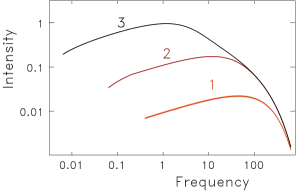
Figure 1: The shape of normalized spectra, $(d{\cal E}_{\rm rad}/d\omega^{\prime})\cdot[4\omega_{c0}/(m_{e}c^{2}\sqrt{1+{\bf a}^{2}})]$, versus the normalized frequency, $\omega^{\prime}/\omega_{c0}$, for different pulse duration. The figure is scalable, particular choice of physical parameters, may be the following: $|{\bf a}|=50$, ${\cal E}=180$ MeV, pulse durations are: 5 fs (curve 1), 36 fs (curve 2) and 220 fs (curve 3). The spectrum broadening and softenning is due to the radiation reaction. In the absence of this reaction curve 1 without changing its shape would scale proportionally to the pulse duration. A zero value of $\log\omega^{\prime}$ corresponds to $\approx 150$ keV.

II.3 Numerical model

Now we introduce the following normalized variables:

$$\tilde{t}=\omega t,\qquad\tilde{{\bf x}}=\omega{\bf x}/c,\qquad\tilde{\bf u}=\frac{\bf u}{c},$$

$$\tilde{\bf E}=\frac{|e|{\bf E}}{m_{e}c\omega},\qquad\tilde{\bf B}=\frac{|e|{\bf B}}{m_{e}c\omega},\qquad\tilde{\bf j}=\frac{4\pi|e|{\bf j}}{m_{e}c\omega^{2}}.$$

Note that the electric current density, $\tilde{\bf j}$ is normalized per $|e|n_{\rm cr}c$, where $n_{\rm cr}=m_{e}\omega^{2}/(4\pi e^{2})$ is the critical density. Below, we use these dimensionless variables and omit tildes in notations. The equations of motion for electrons and positrons read:

$$\frac{d{\bf p}_{e,p}}{dt}={\bf f}_{Le,p}\mp[\bar{\bf u}_{e,p}\times{\bf B}]-{\bf u}_{e,p}{\cal E}_{e,p}^{2}\left({\bf f}_{Le,p}\cdot\bar{\bf u}_{e,p}\right),$$

$$\frac{d{\bf x}_{e,p}}{dt}={\bf u}_{e,p}+\bar{\bf u}_{e,p},\quad{\cal E}_{e,p}=\sqrt{1+{\bf p}^{2}_{e,p}},\quad{\bf u}_{e,p}=\frac{{\bf p}_{e,p}}{\cal E}_{e,p},$$

the normalized Lorentz force and $\bar{\bf u}$ being:

$${\bf f}_{Le,p}=\mp\left({\bf E}+[{\bf u}_{e,p}\times{\bf B}]\right),\qquad\varepsilon=\tau_{0}\omega=\frac{2}{3}\alpha^{3}\omega_{\rm 2Ry}$$

$$\bar{\bf u}_{e,p}=\varepsilon\frac{{\bf f}_{Le,p}-{\bf u}_{e,p}({\bf u}_{e,p}\cdot{\bf f}_{Le,p})}{1+\varepsilon({\bf u}_{e,p}\cdot{\bf f}_{Le,p})}.$$ (29)

For reference we also provide the energy equation:

$$\frac{d{\cal E}_{e,p}}{dt}=\mp\left(\left[{\bf u}_{e,p}+\bar{\bf u}_{e,p}\right]\cdot{\bf E}\right)-{\cal E}_{e,p}^{2}\left({\bf f}_{Le,p}\cdot\bar{\bf u}_{e,p}\right),$$ (30)

For ions with the charge number, $Z$, and the mass, $M_{i}$, the momentum is normalized per $M_{i}c$, so that in their equation of motion the electron-to-ion mass ratio comes:

$$\frac{d{\bf p}_{i}}{dt}=\frac{Z}{M_{i}/m_{e}}\left({\bf E}+[{\bf u}_{i}\times{\bf B}]\right),$$ (31)

$$\frac{d{\bf x}_{i}}{dt}={\bf u}_{i},\qquad{\bf u}_{i}=\frac{{\bf p}_{i}}{\sqrt{1+{\bf p}^{2}_{i}}}.$$ (32)

Below we assume that $Z=1$ and $M_{i}=M_{p}$ is the proton mass. The normalized Maxwell equations read:

$$\frac{\partial{\bf E}}{\partial t}+{\bf j}=\nabla\times{\bf B},\qquad\frac{\partial{\bf B}}{\partial t}=-\nabla\times{\bf E}.$$ (33)

II.3.1 Macroparticles and their current

We assume that the rectangular grid splits the computational domain into the control volumes (cells), $\Delta V=\prod{\Delta x}_{k}$. If the electron density equals $n_{\rm cr}$, there are $n_{\rm cr}\Delta V$ electrons per cell. The latter number is typically very large, so that the plasma electrons cannot be simulated individually and they are combined into macroparticles with a large number of “electrons-per-particle”, $N_{epp}$. In a plasma of critical density the number of (macro)particles per cell is: $N_{ppc}=n_{\rm cr}\Delta V/N_{epp}$.

The electron current density inside the given cell is expressed in terms of the sum over electron macroparticles in this cell. As long as the electric current density is normalized per $n_{\rm cr}c$, the contribution to the latter sum from each macroparticle equals $-(1/N_{ppc})d{\bf x}_{e}/dt$. On adding the contributions from positrons and protons, we obtain:

$${\bf j}=\frac{-\sum_{e}{({\bf u}_{e}+\bar{\bf u}_{e})}+\sum_{p}{({\bf u}_{p}+\bar{\bf u}_{p})}+\sum_{i}{{\bf u}_{i}}}{N_{ppc}}.$$ (34)

II.3.2 Energy integral and energy balance.

We now establish the relationship between the energy integral and the finite sum which represents this integrals in simulations. Particularly, the field energy may be calculated as the total of point-wise field magnitudes squared: ${\cal E}_{\rm field}=\frac{1}{2}\sum_{cells}{({\bf E}^{2}+{\bf B}^{2})},$ which is by a factor of ${\cal E}_{0}=m_{e}c^{2}(n_{\rm cr}\Delta V)$ different from the dimensional field energy. Now consider the total plasma energy, which includes the particle energy as well:

$${\cal E}_{\rm plasma}={\cal E}_{\rm field}+\frac{\sum_{cells}{\left(\frac{M_{i}}{m_{e}}\sum_{i}{\cal E}_{i}+\sum_{e}{\cal E}_{e}+\sum_{p}{\cal E}_{p}\right)}}{N_{ppc}}.$$

Eqs.(30,33,34) give: $d({\cal E}_{\rm plasma}+{\cal E}_{\rm rad})/dt=0,$ where

$$\frac{d{\cal E}_{\rm rad}}{dt}=\frac{\sum_{cells}{\sum_{e,p}{{\cal E}^{2}_{e,p}\left({\bf f}_{Le,p}\cdot\bar{\bf u}_{e,p}\right)}}}{N_{ppc}}$$ (35)

is the radiation energy loss rate. Therefore, the contribution from electrons and positrons to the dimensionless radiation energy at each time step, $\Delta t$, is calculated as ${\cal E}^{2}_{e,p}\left({\bf f}_{Le,p}\cdot\bar{\bf u}_{e,p}\right)\Delta t/N_{ppc}$. Once integrated over the simulation time, the radiation energy may be converted to physical units on multplying it by a factor of ${\cal E}_{0}$.

II.3.3 Algorithmic implementation

The algorithmic changes to the standard PIC scheme are minimal as long as we ignore the radiation transport and only integrate over time the energy emitted by electrons (and positrons, if any). To collect the radiation, we introduce the energy bins (an array) ${\cal E}_{{\rm rad}\,ijk}(\log(\bar{\omega})_{i},\theta_{j},\varphi_{k})$, which discretize the modified frequency-angular spectrum of emission. Inside the desired interval of the photon energies we introduce the logarithmic grid, $\log(\bar{\omega})_{i}$, equally spaced with the step, $\Delta\log(\bar{\omega})$. We also introduce a grid, $\theta_{j},\varphi_{k}$, for the two polar angles of the spherical coordinate system, with $\Delta{\bf n}_{jk}$ being the element of solid angle: $\Delta{\bf n}_{jk}=\sin(\theta_{j})\Delta\theta\Delta\varphi$.

To calculate both the spectrum of emission and the radiation back-reaction we modify only that part of the PIC algorithm which accounts for the electron motion. Specifically, we employ the standard leapfrog numerical scheme which involves, among others, the following stages: (1) for each electron macroparticle, update momentum through the time step by adding the Lorentz force, following the Boris scheme: ${\bf p}^{n+1/2}_{e}={\bf p}^{n-1/2}_{e}+\Delta t\ {\bf f}_{Le}({\bf E}^{n},{\bf B}^{n})$; (2) solve the energy and the velocity from the updated momentum: ${\cal E}^{n+1/2}_{e}=\sqrt{1+({\bf p}^{n+1/2})^{2}_{e}}$, ${\bf u}^{n+1/2}_{e}={\bf p}^{n+1/2}_{e}/{\cal E}^{{n+1/2}}_{e}$; (3) use the calculated velocity to update the particle coordinates: ${\bf x}^{n+1}_{e}={\bf x}^{n}_{e}+{\bf u}^{n+1/2}_{e}\Delta t$ and account for the contribution of the electric current element, $-{\bf u}^{n+1/2}_{e}\Delta t$, to the Maxwell equations. Again, these stages are standard and may be found in birdsall . We introduced new steps into this algorithm between stages (2) and (3) as follows.

• Once stage (2) is done, recover the Lorentz force: ${\bf f}_{Le}=({\bf p}^{n+1/2}-{\bf p}^{n-1/2})/\Delta t$.

• Find $\chi=\frac{3}{2}\omega_{\rm 2Ry}\alpha^{2}{\cal E}^{n+1/2}\sqrt{{\bf f}^{2}_{Le}-({\bf f}_{Le}\cdot{\bf u}^{n+1/2})^{2}}$.

• Find $\bar{\bf u}_{e}$ by putting ${\bf f}_{Le}$ and ${\bf u}_{e}^{n+1/2}$ into Eq.(29).

• Calculate $\omega_{c}={\cal E}^{n+1/2}_{e}\chi$ and find the discrete value of $\log(\bar{\omega})_{i}$ most close to $\log{\omega_{c}}$. Find the angles, $\theta_{j},\varphi_{k}$ closest to the direction of ${\bf p}^{n+1/2}$. Add the radiation energy into the proper bin

  $${\cal E}_{{\rm rad}\,ijk}\rightarrow{\cal E}_{{\rm rad}\,ijk}+\frac{({\cal E}^{n+1/2})^{2}({\bf f}_{Le}\cdot\bar{\bf u}_{e})\Delta t}{\omega_{c}N_{ppc}\Delta\log(\bar{\omega})\Delta{\bf n}_{jk}}.$$

• Add the radiation force: ${\bf p}_{e}^{n+1/2}\rightarrow{\bf p}_{e}^{n+1/2}+\Delta t\left\{-[\bar{\bf u}_{e}\times{\bf B}^{n}]-{\bf u}_{e}^{n+1/2}({\cal E}^{n+1/2}_{e})^{2}({\bf f}_{L{e}}\cdot\bar{\bf u}_{e})\right\}$.

• Find ${\bf u}^{n+1/2}_{e}={\bf p}_{e}^{n+1/2}/\sqrt{1+({\bf p}_{e}^{n+1/2})^{2}}+\bar{\bf u}_{e}$ and use this velocity through stage (3).

Note that the algorithm modification is applied only to electrons (positrons), keeping unchanged the ion motion as well as the fields.

The frequency-angular spectrum may be reduced to the frequency one: ${\cal E}_{{\rm rad}\,i}=\sum_{jk}{{\cal E}_{{\rm rad}\,ijk}\Delta{\bf n}_{jk}}$, to the angular one: ${\cal E}_{{\rm rad}\,jk}=\sum_{i}{{\cal E}_{{\rm rad}\,ijk}\bar{\omega}_{i}\Delta\log(\bar{\omega})}$ or to the total radiation energy: ${\cal E}_{\rm rad}=\sum_{ijk}{{\cal E}_{{\rm rad}\,ijk}\bar{\omega}_{i}\Delta\log(\bar{\omega})}\Delta{\bf n}_{jk}$.

While postprocessing the results, we apply the convolution transformation, (15), to the radiation spectrum and multiply it by ${\cal E}_{0}$. The resulting spectrum, $d{\cal E}_{\rm rad}/(d{\bf n}d\omega^{\prime})$, is a function of $\log[\hbar\omega^{\prime}/(m_{e}c^{2})]$.

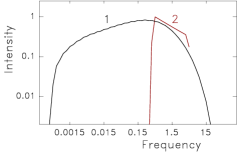
Figure 2: Test simulation result: (a): radiation energy spectrum (line 1), $d{\cal E}_{\rm rad}/d\omega^{\prime}$, and the modified spectrum, $d{\cal E}_{\rm rad}/d\bar{\omega}$ (line 2); (b),(c): the angular distribution of the radiation at instants: (b) t=1T, (c) t=100T, where $T=2\pi/\omega$.

II.4 Simulation result

The analytical solution presented in Sec.II.2 has been used to benchmark the numerical scheme. In the test simulation electrons with an initial momentum, $p_{\|}=300$, propagate toward the laser pulse with sharp (2$\lambda$) fronts. The circularly polarized laser pulse has amplitude, $|{\bf a}|=15$, and duration, $100(2\pi/\omega)$. Interacting with the pulse, the particles radiate energy, finally approaching momentum of $p_{\|}\approx 130$.

In Fig.2(a) the spectrum of the resulting radiation $d{\cal E}_{\rm rad}/d\omega^{\prime}$ is shown. We also provide the modified spectrum (the distribution over $\bar{\omega}=\omega_{c}$), which is close to satisfying a power law, and in a full agreement with the analytical solution. In Fig.2(b)-(c) typical evolution of the angular radiation distribution, $d{\cal E}_{\rm rad}/d{\bf n}$, is provided for the same simulation. One can see that the majority of the radiation is concentrated in a narrow angle with respect to the direction of backscattered light (0^o). A softer part of the radiation exhibits a wider angular distribution and becomes less intense [Fig. 2(c)].

III QED-moderate fields ($\chi\sim 1$)

When $\chi$ is not small ($J\sim 3\cdot 10^{3}{\rm W/cm}^{2}$), QED effects come into play. Here we describe how to extend the methods used above towards finite $\chi$. This is achieved by applying realistic QED spectra of emission as derived in Ref.PRE , with the radiation force modified accordingly.

This approach is applicable as long as we ignore the onset of some new effects which are only pertinent to QED-strong fields. Specifically, while employing the radiation force, $dp^{\mu}_{\rm rad}/d\tau$, it is admitted that the change in the electron momentum, $d\tau\cdot dp^{\mu}_{\rm rad}/d\tau$, within the infinitesimal time interval, $d\tau$, is also infinitesimal. This ’Newton’s law’ approximation is pertinent to classical physics and it ignores the point that the change in the electron momentum at $\chi\sim 1$ is essentially finite because of the finite momentum of emitted photon. The approximation, however, is highly efficient and allows one to avoid time-consuming statistical simulations. Its error tends to zero as $\chi\rightarrow 0$, and it is sufficiently small at $\chi\sim 1$.

Another effect which we ignore in this section is the pair production due to $\gamma$-photon absorption in the strong laser field. This neglect allows us to avoid solving the computationally intense radiation transport problem.

III.1 Theoretical notes

III.1.1 Emission spectrum

The emission probability found in Ref.PRE within the framework of QED can be reformulated in a form similar to Eq.(9). The polarized part of emission may be reduced to Eq.(9) with the modified vector amplitude:

$${\bf A}_{\rm QED}(\omega^{\prime})=\sqrt{\frac{1}{C_{fi}}}{\bf A}_{\rm cl}\left(\frac{\omega^{\prime}}{C_{fi}}\right),\qquad C_{fi}=\frac{(k\cdot p_{i})}{(k\cdot p_{f})},$$

subscript $i$ and $f$ denoting the parameters of an electron prior to and after the emission of a single photon, and:

$$\frac{dI_{\rm QED}^{\rm pol}(\omega^{\prime})}{d\omega^{\prime}}=C_{fi}\frac{dI_{\rm cl}(\frac{\omega^{\prime}}{C_{fi}})}{d\omega^{\prime}}=\frac{C_{fi}I_{\rm cl}}{\omega_{c}}Q_{\rm cl}\left(\frac{r}{C_{fi}}\right).$$ (36)

Within the framework of QED the electron possesses not only an electric charge, but also a magnetic moment associated with its spin. Usually the spin is assumed to be depolarized (as is done in Ref.PRE ), and, accordingly, a depolarized contribution to the emission appears:

$$\frac{dI^{\rm depol}_{\rm QED}}{d\omega^{\prime}}=\frac{I_{\rm cl}(\tau)}{\omega_{c}}\frac{9\sqrt{3}}{8\pi}\left(1-C_{fi}\right)^{2}\frac{r}{C_{fi}}K_{2/3}\left(\frac{r}{C_{fi}}\right).$$ (37)

Thus, the QED effect in the emission from an electron in a strong electromagnetic field reduces to a downshift in frequency accompanied by an extra contribution from the magnetic moment of electron. The universal emission spectrum in QED-strong fields is given by the total of Eqs.(36,37):

$$\frac{dI_{\rm QED}}{d\omega^{\prime}}=\frac{I_{\rm cl}}{\omega_{c}}q(\chi)Q_{\rm QED}(r,\chi),\quad I_{\rm QED}=I_{\rm cl}q(\chi),$$

where $Q_{\rm QED}=Q^{\prime}_{\rm QED}/q$ is the normalized by unity spectrum, $q(\chi)=\int_{0}^{\infty}{Q^{\prime}_{\rm QED}(r,\chi)dr}\leq 1$ is the normalization parameter, the spectrum before normalization is:

$$Q^{\prime}_{\rm QED}(r,\chi)=\frac{9\sqrt{3}}{8\pi}r\left[\int\limits_{r_{\chi}}^{\infty}{K_{5/3}(r^{\prime})dr^{\prime}}+\chi^{2}rr_{\chi}K_{2/3}(r_{\chi})\right],$$

and $r_{\chi}=r/(1-\chi r)$.

Figure 3: Emission spectra for various values of $\chi$.

Figure 4: Emitted radiation power in the QED approach vs classical (solid); an interpolation formula $I_{\rm QED}=I_{\rm cl}/(1+1.04\sqrt{I_{\rm cl}/I_{C}})^{4/3}$ (dashed). Here, $I_{C}=I_{\rm cl}/\chi^{2}$.

III.1.2 Equation for electron motion: accounting the radiation back-reaction.

As long as the QED effects modify emission,

$$Q_{\rm cl}(r)\rightarrow Q_{\rm QED}(r,\chi),\qquad I_{\rm cl}\rightarrow I_{\rm QED},$$ (38)

the radiation back-reaction needs to be revised accordingly. In Refs.mine ; our it was noted, that QED is not compatible with the traditional approach to the radiation force in classical electrodynamics, while Eqs.(16,17) may be employed at finite value of $\chi$ on substituting $I_{\rm QED}$ for $I_{\rm cl}$. Alternatively, within the framework of QED the radiation back-reaction may be found by integrating the 4-momentum carried away with the emitted photons and that absorbed from the external electromagnetic field in the course of emission. For a 1D wave field this procedure gives the following equation (see Ref.PRE ):

$$\frac{dp^{\alpha}}{d\tau}=\frac{f^{\alpha}_{Le}}{m_{e}c}+\frac{I_{\rm QED}}{m_{e}c^{2}}\left[\frac{k^{\alpha}}{(k\cdot p)}-p^{\alpha}\right],$$ (39)

and in such field $F^{\alpha\beta}F_{\beta\mu}p^{\mu}/(p_{\nu}F^{\nu\beta}F_{\beta\mu}p^{\mu})=k^{\alpha}/(k\cdot p)$, $k^{\alpha}$ being the wave 4-vector. Eq.(39) coincides with Eqs.(16,17), in which the substitution (38) is made, or, the same, the three-vector formulation for $\bar{\bf u}$ is applicable to the 1D wave field, if the substitution is done as follows:

$$\tau_{0}\rightarrow\tau_{0}\frac{I_{\rm QED}}{I_{\rm cl}}=\tau_{0}q(\chi).$$ (40)

Although this approach is derived for the 1D field, we may apply it to an arbitrary 3D focused field. An argument in favor of this generalization is that the property of a 1D wave, $(k\cdot k)=0$, which is used while deriving Eq.(39), holds as an approximation for any field. Indeed, on calculating the 4-square of $F^{\alpha\beta}F_{\beta\mu}p^{\mu}/(p_{\nu}F^{\nu\beta}F_{\beta\mu}p^{\mu})$, which 4-square is similar to $(k\cdot k)/(k\cdot p)^{2}$, we find:

$$\frac{p\cdot F^{4}\cdot p}{(p\cdot F^{2}\cdot p)^{2}}=\frac{9}{4}\chi^{-2}\frac{E^{2}-B^{2}}{E_{S}^{2}}+\frac{81}{16}\chi^{-4}\frac{({\bf E}\cdot{\bf B})^{2}}{E_{S}^{4}}\ll 1,$$

the inequality holds at $\chi\geq 1$ according to Ineq.(7).

Another criterion which should be checked at $\chi\geq 1$ is the requirement for the difference, $(1-u^{2})\propto\chi^{2}$, as in Eq.(22) to be small. Applying the substitution (40) to (22) we find that $(1-u^{2})\leq 2\cdot 10^{-6}$, reaching its maximal value at $\chi\sim 3.4$. This ’error’ is negligible, even if one assumes, than any theory allowing $u^{2}\neq 1$, is erroneous.

III.2 Analytical result

In Fig.5 we show the emission spectrum for an electron interacting with a laser pulse (see PRE for detail). We see that the QED effects essentially modify the spectrum even with laser intensities which are already achieved.

Figure 5: The emission spectrum for 600 MeV electrons interacting with 30-fs laser pulses of intensity $2\cdot 10^{22}W/cm^{2}$: with (solid) or without (dashed) accounting for the QED effects. Here $\hbar\omega_{c0}\approx 1.1$ MeV for $\lambda=0.8\mu$m.

III.3 Numerical model.

As long as the QED spectrum of emission depends on $\chi$, the bins for collecting the radiation energy should be refined: ${\cal E}_{{\rm rad}\,ijkl}(\bar{\omega}_{i},{\bf n}_{jk},\chi_{l})$. Once for a given electron (or positron) the parameter $\chi$ is calculated; the discrete value of $\chi_{l}$ should be found most close to $\chi$. Then, parameter $\varepsilon$ should be found following Eq.(40), $\varepsilon=q_{l}\tau_{0}\omega$, using pre-tabulated value, $q_{l}=q(\chi_{l})$. Then, $\bar{\bf u}_{e}$ should be expressed in terms of $\varepsilon$ and the radiated energy should be added to a proper energy bin:

$${\cal E}_{{\rm rad}\,ijkl}\rightarrow{\cal E}_{{\rm rad}\,ijkl}+\frac{({\cal E}^{(n+1/2)}_{e})^{2}({\bf f}_{Le}\cdot\bar{\bf u}_{e})\Delta t}{\omega_{c}N_{ppc}\Delta\log(\bar{\omega})\Delta{\bf n}_{jk}}.$$

While postprocessing the results, a convolution similar to (15) should be applied with $\chi_{l}$-dependent spectra:

$$\frac{d{\cal E}_{\rm rad}(\omega^{\prime},{\bf n})}{d{\bf n}d\omega^{\prime}}={\cal E}_{0}\sum_{\chi_{l}}{\int{Q_{\rm QED}\left(\frac{\omega^{\prime}}{\bar{\omega}},\chi_{l}\right){\cal E}_{{\rm rad}\,ijkl}d\log\bar{\omega}}}.$$

III.4 Simulation results

Figure 6: Backscattered light in simulation of the interaction of laser pulse of intensity $2\times 10^{23}$W/cm² with plasma of density $6.5\times 10^{22}$cm^-3. For each $\chi_{l}$ (vertical axis) the convolution integral (the term in the above formula for convolution) is calculated and presented as a function of $\hbar\omega^{\prime}$ (horizontal axis). The line shows the total emitted energy as a function of the cutoff photon energy (i.e. the integral spectrum).

In a 1D simulation presented in Fig.6 a linearly polarized laser pulse with a step-like profile having 2-$\lambda$ front and amplitude $a=300$ interacts with plasma of density $n_{0}=30n_{c}$ during 50 cycles. About half of laser energy is converted to high energy photons. The data for backscattered photons indicate that values of $\chi\approx 1$ are achieved. These values are reasonable, as the energy of electrons moving toward the pulse is as high as 180MeV, and the vector potential approach values $a=400$ due to superposition of incident and reflected light. One can see that $\sim$65% of emitted photons exceed 10MeV, and 96% are above 1MeV.

IV QED-strong fields ($\chi\gg 1$)

IV.1 Theoretical notes

In cases where $\chi\gg 1$ one needs to solve the RTE in order to account for $\gamma$-photon absorption in strong fields. This may be done using the Monte-Carlo method, in which the radiation field is evaluated statistically (see Refs.nay09 ; mas09 ; bae09 ). Instead of the radiation energy density the photon distribution function may be introduced as follows:

$$f_{\gamma}({\bf x},\omega^{\prime},{\bf n})=\frac{{\cal I}({\bf x},\omega^{\prime},{\bf n})}{m_{e}c^{2}\omega^{\prime}}.$$ (41)

Similar to the way the electron macroparticles represent the electron distribution function, the photon marcoparticles may be employed to simulate the photon distribution function. To simulate emission, the photons are created with their momentum selected statistically. The photon propagation in the direction of ${\bf n}$ is simulated in the same way as for electrons. The absorption with the known probability is also simulated statistically.

Now we may split the radiation for the part which may be treated in the way we followed so far (see Sec.II-III) and for the Monte-Carlo photons. We choose a parameter, $\chi^{*}\sim(0.05-1)$ and assume that: (1) an electon with $\chi\leq\chi^{*}$ contributes only to $d{\cal E}_{\rm rad}/(d\omega^{\prime}d{\bf n})$; while (2) for an electron with $\chi>\chi^{*}$ the regular spectrum of emission, $Q^{\prime}_{\rm QED}(r,\chi)$ (which is normally truncated at $r=1/\chi$), is now truncated at $r=\chi^{*}/\chi^{2}<1/\chi$ and the emission of photons with $\chi^{*}/\chi^{2}\leq r\leq\chi$, or, the same, $\frac{\chi^{*}}{\chi}\leq\frac{\omega^{\prime}}{{\cal E}}\leq 1,$ is treated statistically. The regular radiation loss rate as well as the contribution to the radiation force $\propto-{\bf p}I_{\rm QED}$ should be both reduced by a factor of $q_{t}(\chi)/q(\chi)$ at $\chi>\chi^{*}$, where the truncated spectrum integral equals: $q_{t}(\chi)=\int_{0}^{\chi^{*}/\chi^{2}}{Q^{\prime}_{\rm QED}(r,\chi)dr}$. The normalized by unity trucnated spectrum is: $Q_{t}(r,\chi)=\frac{q(\chi)Q_{\rm QED}(r,\chi)}{q_{t}(\chi)},\,r<\chi^{*}/\chi^{2}$. The emission probability to be used at $\chi>\chi^{*}$, $r>\chi^{*}/\chi^{2}$ may be found in PRLsuppl :

$$dW_{e\rightarrow e,\gamma}=\frac{\kappa K_{2/3}(r_{\chi})+\int\limits_{r_{\chi}}^{\infty}{K_{5/3}(r^{\prime})dr^{\prime}}}{\pi\sqrt{3}\alpha\omega_{\rm 2Ry}}d\left(\frac{\omega^{\prime}}{{\cal E}}\right)\frac{d(\omega t)}{{\cal E}},$$

where $r_{\chi}=\frac{\omega^{\prime}/{\cal E}}{\chi(1-\omega^{\prime}/{\cal E})}$, $\kappa=\frac{(\omega^{\prime}/{\cal E})^{2}}{1-\omega^{\prime}/{\cal E}}$ and for a 1D wave field we use an equation, $\frac{d(\omega t)}{\sqrt{3}\alpha\omega_{\rm Ry}}=\frac{\sqrt{3}\alpha d\xi}{2\chi}\left|\frac{d{\bf a}}{d\xi}\right|$. If the emission probability is averaged over time or over an ensemble, we return to the above spectrum of emission: $\omega^{\prime}m_{e}c^{2}\left<dW_{e\rightarrow e,\gamma}/(drdt)\right>=I_{\rm QED}Q_{\rm QED}(r,\chi)$, Here we apply the formula, $\frac{1}{\sqrt{3}\alpha\omega_{\rm Ry}}=\frac{9\sqrt{3}I_{\rm QED}}{8\chi^{2}q(\chi)\omega m_{e}c^{2}}$, which is also used in the numerical scheme.

IV.2 Semi-analytical solution

In ourPRL we demonstrated that as long as the distribution functions, $f_{e,p,\gamma}$, for electrons, positrons and photons in a 1D wave field are integrated over the transversal components of momentum, their evolution is described by simple kinetic equations with the collision integrals. We solved these equation numerically. This choice of initial conditions corresponds to the 46.6 GeV SLAC electron beam and the laser intensity of $J\approx 5\cdot 10^{22}\,{\rm W/cm}^{2}$ for $\lambda=0.8\mu$m, to be achieved soon. As long as the Monte-Carlo method is not used, the numerical results, such as the total pair production, may be used to benchmark the numerical scheme described here.

IV.3 Numerical model

The modification of the numerical scheme as used in Sec.III is needed only for electrons and positrons with $\chi>\chi^{*}$. The radiation energy added to the proper energy bin is corrected as follows:

$${\cal E}_{{\rm rad}\,ijkl}\rightarrow{\cal E}_{{\rm rad}\,ijkl}+\frac{q_{t}(\chi_{l})}{q(\chi_{l})}\frac{({\cal E}^{(n+1/2)}_{e})^{2}({\bf f}_{Le}\cdot\bar{\bf u}_{e})\Delta t}{\omega_{c}N_{ppc}\Delta\log(\bar{\omega})\Delta{\bf n}_{jk}},$$

and the same correction factor is applied to the second term in braces at algorithm stage 2.5. After stage 2.5 a probable hard photon emission from the electron with $\chi>\chi^{*}$ is accounted, using the probability:

$$\frac{dW_{e\rightarrow e,\gamma}}{d(\omega^{\prime}/{\cal E})}=\delta w\left(\frac{\omega^{\prime}}{\cal E},\chi\right),\quad\delta=\frac{({\cal E}^{(n+1/2)}_{e})^{2}({\bf f}_{Le}\cdot\bar{\bf u}_{e})\Delta t}{\chi^{2}{\cal E}^{(n+1/2)}},$$

$$w\left(\frac{\omega^{\prime}}{\cal E},\chi\right)=\frac{9\sqrt{3}}{8\pi q(\chi)}\left[\kappa K_{2/3}(r_{\chi})+\int\limits_{r_{\chi}}^{\infty}{K_{5/3}(r^{\prime})dr^{\prime}}\right],$$

The total probability of emission is given by a complete integral: $W_{e\rightarrow e,\gamma}=\delta\int_{\chi^{*}/\chi}^{1}{w\left(\frac{\omega^{\prime}}{\cal E},\chi\right)d\left(\frac{\omega^{\prime}}{\cal E}\right)}$. Both within the QED perturbation theory and within the Monte-Carlo scheme $W_{e\rightarrow e,\gamma}$ is assumed to be less than one. The probability of no emission equals $1-W_{e\rightarrow e,\gamma}\geq 0$. The partial probability, $W_{e\rightarrow e,\gamma}(\omega^{\prime}<\omega^{\prime}_{0})$, for the emission with the photon energy not exceeding the given value, $\omega^{\prime}_{0}$, is given by the incomplete probability integral:

$$W_{e\rightarrow e,\gamma}(\omega^{\prime}<\omega^{\prime}_{0})=\delta\int_{\chi^{*}/\chi}^{\omega^{\prime}_{0}/{\cal E}}{w\left(\frac{\omega^{\prime}}{\cal E},\chi\right)d\left(\frac{\omega^{\prime}}{\cal E}\right)}$$

Therefore, for given $\delta$ and $\chi$ and for a randomly generated number, $0\leq{\rm rnd}<1$ one can solve $\omega^{\prime}/{\cal E}$ from an integral equation as follows (see detail in Appendix B):

$$\int^{\omega^{\prime}/{\cal E}}_{\chi^{*}/\chi}{w\left(z,\chi\right)dz}=\frac{\rm rnd}{\delta}\leq\int^{1}_{\chi^{*}/\chi}{w\left(z,\chi\right)dz},$$ (42)

if the gambled value of ${\rm rnd}$ does not exceed $W_{e\rightarrow e,\gamma}$: $0\leq{\rm rnd}\leq W_{e\rightarrow e,\gamma}$. Otherwise (if $W_{e\rightarrow e,\gamma}<{\rm rnd}\leq 1$) the extra emission does not occur. With calculated $\omega^{\prime}/{\cal E}$, the emission is accounted for by creating a new photon macroparticle with the momentum, ${\bf p}^{(n+1/2)}_{e}(\omega^{\prime}/{\cal E})$ and an electron recoil is accounted for by reducing the electron momentum, ${\bf p}^{(n+1/2)}_{e}\rightarrow{\bf p}^{(n+1/2)}_{e}(1-(\omega^{\prime}/{\cal E}))$.

IV.3.1 Photon propagation and absorption

The new element of the numerical scheme is the photon macroparticle, which simulates $(n_{\rm cr}\Delta V)/N_{ppc}$ real photons. Its propagation with dimensionless velocity equal to ${\bf n}$ is treated in the same way as for electrons and ions.

If the photon escapes the computational domain, its energy should be accounted for while calculating the total emission from plasma. For this purpose we introduce the energy bins, ${\cal E}^{(tot)}_{{\rm rad}\,ijk}(\log({\omega^{\prime}})_{i},\theta_{j},\varphi_{k})$, such that the logarithmic equally spaced grid for the photon energy, $\log({\omega}^{\prime})_{i}$, and the polar angle grid coincide with those introduced above. The contribution from the escaping photon with total energy, $\omega^{\prime}m_{e}c^{2}n_{\rm cr}\Delta V/N_{ppc}$, should be added to the bin with the closest $\log({\omega^{\prime}})_{i},\theta_{j},\varphi_{k}$, with the macroparticle energy being converted to the spectral energy density by dividing by $\Delta\omega^{\prime}=\omega^{\prime}\Delta\log({\omega^{\prime}})$:

$${\cal E}^{(tot)}_{{\rm rad}\,ijk}\rightarrow{\cal E}^{(tot)}_{{\rm rad}\,ijk}+\frac{m_{e}c^{2}(n_{\rm cr}\Delta V)}{N_{ppc}\Delta\log({\omega^{\prime}})}$$

The photon absorption with electron-positron-pair creation is gambled in the same way as the emission (see details in Appendix B). Other absorption mechanisms may be also included. In postprocessing the simulation results, the softer $\gamma$-photon emission should be added to the total radiation spectrum:

$$\frac{d{\cal E}_{\rm rad}(\omega^{\prime},{\bf n})}{d{\bf n}d\omega^{\prime}}={\cal E}^{(tot)}_{{\rm rad}\,ijk}+m_{e}c^{2}(n_{\rm cr}\Delta V)\times$$

$$\times\sum_{\chi_{l}}{\int{Q_{t}\left(\frac{\omega^{\prime}}{\bar{\omega}},\chi_{l}\right){\cal E}_{{\rm rad}\,ijkl}d\log\bar{\omega}}}$$

IV.4 Simulation result

Repeating the test simulation as described in Sec.III.D and applying the Monte-Carlo scheme at $\chi>\chi^{*}=0.1$, and without photon absorption, we notice only an increase in the fluctuations of the high-energy portion of the radiation spectrum. In this region, the photons are statistically underrepresented, the number of particles per $\Delta\log(\omega^{\prime})$ being small.

V Conclusion

Thus, the range of field intensities which may be simulated with good accuracy using the described tools is now extended towards the intensities as high as $(2-3)\cdot 10^{23}{\rm W/cm}^{2}$. In such fields, which are typical for the radiation-dominated regime of the laser-plasma interaction, the suggested scheme is validated against a semi-analytical solution. Different versions of the equation of the emitting particle motion are compared and their proximity is demonstrated.

Extension of the model for QED-strong fields can be easily incorporated into the scheme. The emission spectra are substantially modified by QED effects and simulation results for a realistic laser-plasma interaction are provided.

For the QED-strong field regime of laser-plasma interaction the Monte-Carlo method should be used to simulate emission-absorption of harder $\gamma$-photons. Although such simulations are doable (see ner11 ), more work on the scheme validation is needed.

Appendix A. MacDonald functions

The MacDonald functions allow solutions for the following integrals:

$$\int\limits_{-\infty}^{+\infty}{\cos\left[\frac{3}{2}r\left(\frac{z^{3}}{3}+z\right)\right]dz}=\frac{2}{\sqrt{3}}K_{1/3}(r),$$

(see Eq.(8.433) in gr )

$$\int\limits_{-\infty}^{+\infty}{z\sin\left[\frac{3}{2}r\left(\frac{z^{3}}{3}+z\right)\right]dz}=\frac{2}{\sqrt{3}}K_{2/3}(r),$$

$$\int\limits_{-\infty}^{+\infty}{\frac{1}{z}\sin\left[\frac{3}{2}r\left(\frac{z^{3}}{3}+z\right)\right]dz}=-\frac{2}{\sqrt{3}}\int\limits_{r}^{+\infty}{K_{1/3}(r^{\prime})dr^{\prime}},$$

Using the known relationships, $2\frac{dK_{\nu}(r)}{dr}=-K_{\nu-1}(r)-K_{\nu+1}(r),$ $K_{-\nu}(r)=K_{\nu}(r)$, more integrals may be reduced to the MacDonald functions, particularly:

$$\int\limits_{-\infty}^{+\infty}{\frac{1+2z^{2}}{z}\sin\left[\frac{3}{2}r\left(\frac{z^{3}}{3}+z\right)\right]dz}=\frac{2}{\sqrt{3}}\int\limits_{r}^{+\infty}{K_{5/3}(r^{\prime})dr^{\prime}}.$$

The advantage of the MacDonald functions is the fast convergence of their integral representation:

$$K_{\nu}(r)=\int_{0}^{\infty}{\exp\left[-r\cosh(z)\right]\cosh(\nu z)dz},$$

$$\int_{r}^{\infty}{K_{\nu}(r^{\prime})dr^{\prime}}=\int_{0}^{\infty}{\exp\left[-r\cosh(z)\right]\frac{\cosh(\nu z)}{\cosh(z)}dz},$$

(see Eq.(8.432) in gr ). In numerical simulations, therefore, the MacDonald functions may be calculated by integrating their representations using the Simpson method, unless the argument, $z$, is very small or very large, in which case one can employ the series and asymptotic expansions for cylindrical functions (see gr ).

Appendix B. Event generator for emission

To solve Eq.(42) numerically, one needs to pre-calculate the table:

$$W_{ml}=\int^{(\omega^{\prime}/{\cal E})_{m}}_{\chi^{*}/\chi}{w\left(z,\chi_{l}\right)dz}$$

for discrete $\chi_{l}$ and for discrete uniformly spaced values of $(\omega^{\prime}/{\cal E})_{m}\leq 1$. For known $\chi_{l}>\chi^{*}$ the positive value of $W_{ml}$ most close to ${\rm rnd}/\delta$ determines the value of $(\omega^{\prime}/{\cal E})_{m}$.

For the absorption probability we use an analogous formule from PRLsuppl :

$$dW_{\gamma\rightarrow e,p}=\frac{\kappa K_{2/3}(r_{\chi})-\int\limits_{r_{\chi}}^{\infty}{K_{5/3}(r^{\prime})dr^{\prime}}}{\pi\sqrt{3}\alpha\omega_{\rm Ry}}d\left(\frac{{\cal E}}{\omega^{\prime}}\right)\frac{d(\omega t)}{\omega^{\prime}},$$

where $r_{\chi}=\frac{1}{\chi_{\gamma}(1-{\cal E}/\omega^{\prime}){\cal E}/\omega^{\prime}}$, $\kappa=\chi_{\gamma}r_{\chi}$. Here, ${\cal E}$ is the energy of the electron created in the $\gamma$-photon absoption together with a positron of energy $\omega^{\prime}-{\cal E}$. The $\chi$-parameter for a photon, $\chi_{\gamma}$, is calculated as for an electron with an energy, $\omega^{\prime}$, and a dimensionless velocity, ${\bf n}$, in terms of the local electromagnetic field intensities.

References

- (1) S.-W. Bahk et al, Opt. Lett. 29, 2837 (2004); V. Yanovsky et al, Optics Express 16, 2109 (2008).
- (2) http://eli-laser.eu/; E. Gerstner, Nature 446, 16 (2007).
- (3) I.V. Sokolov et al, Phys. Plasmas 16, 093115 (2009).
- (4) J. Koga, T. Zh. Esirkepov and S. V. Bulanov, Phys.Plasmas 12, 093106 (2005).
- (5) A. Zhidkov et al, Phys. Rev. Lett. 88, 185002 (2002); Y. Y. Lau et al, Phys. Plasmas 10, 2155 (2003); F. He et al, Phys. Rev. Lett. 90, 055002 (2003); S. V. Bulanov et al, Plasma Phys. Rep. 30, 196 (2004); N. M. Naumova et al, Phys. Rev. Lett. 92, 063902 (2004); N. M. Naumova et al, Phys. Rev. Lett. 93, 195003 (2004); J. Nees et al, J. Mod. Optics 52, 305 (2005); N. M. Naumova, J. A. Nees and G. A. Mourou, Phys. Plasmas 12, 056707 (2005).
- (6) N. M. Naumova et al, Phys. Rev. Lett.,102, 025002 (2009); T. Schlegel et al, Phys. Plasmas, 16, 083103 (2009).
- (7) J. Schwinger, Phys. Rev. 82, 664 (1951); E. Brezin and C. Itzykson, Phys. Rev. D 2, 1191 (1970).
- (8) C. Bula et al, Phys. Rev. Lett. 76, 3116 (1996); D.L. Burke al, Phys. Rev. Lett. 79, 1626 (1997);Bamber, C. et al, Phys. Rev. D, 60, 092004 (1999); M. Marklund and P. K. Shukla, Rev. Mod. Phys. 78, 591 (2006); Y. I. Salamin et al, Phys. Reports 427, 41 (2006); A. M. Fedotov et al, Phys. Rev. Lett. 105, 080402 (2010).
- (9) A.R. Bell and J.G.Kirk, Phys. Rev. Lett. 101, 200403 (2008).
- (10) I.V. Sokolov et al, Phys. Rev. Lett. 105, 195005 (2010).
- (11) J. D. Jackson, Classical Electrodynamics (Wiley, New York, 1999).
- (12) A. Rousse et al, Phys Rev. Lett. 93, 135005 (2004); S. Kiselev, A. Pukhov, and I. Kostyukov, Phys. Rev. Lett. 93, 135004 (2004).
- (13) S. Kneip et al, Proc. SPIE 7359, 73590T (2009).
- (14) L. D. Landau and E. M. Lifshits, The Classical Theory of Fields (Pergamon, New York, 1994).
- (15) I.V. Sokolov et al, Phys. Rev. E 81, 036412 (2010).
- (16) J.L. Martins et al, Proc. SPIE 7359, 73590V (2009).
- (17) A. G. R. Thomas, Phys. Rev. ST Accel. Beams, 13, 020702 (2010).
- (18) Ya.B.Zel’dovich and Yu.P.Raizer, Physics of Shock Waves and High-Temperature Hydrodynamic Phenomena,
- (19) I.V. Sokolov, JETP 109, 207 (2009).
- (20) I. V. Sokolov, N. M. Naumova, J. A. Nees, V. P. Yanovsky, and G. A. Mourou AIP Conf. Proc. 1228, 305 (2010).
- (21) C. K. Birdsall and A. B. Langdon, Plasma Physics via Computer Simulation (McGraw-Hill, New York, 1985).
- (22) Nayakshin, S., Cha, S.H., and Hobbs, A. MNRAS, 397, 1314 (2009).
- (23) Maselli, A., Ferrara, A., and Gallerani, S., MNRAS, 395, 1925 (2009).
- (24) Baek, S., Di Matteo, P., Semelin, B., Combes, F., and Revaz, Y., Astron. and Astrophys., 495, 389 (2009).
- (25) http://link.aps.org/supplemental/10.1103/PhysRevLett. 105.195005; I.V. Sokolov et al., arXiv:1009.0703.
- (26) E. N. Nerush, I. Yu. Kostyukov, A. M. Fedotov, N. B. Narozhny, N. V. Elkina, and H. Ruhl, Laser Field Absorption in Self-Generated Electron-Positron Pair Plasma, Phys. Rev. Lett. 106, 035001 (2011).
- (27) I. S. Gradshtein and I. M. Ryzhik, Table of Integrals, Series, and Products (Academic Press, New York, 1965).