The ExaVolt Antenna: A Large-Aperture, Balloon-embedded Antenna
for Ultra-high Energy Particle Detection

Abstract

We describe the scientific motivation, experimental basis, design methodology, and simulated performance of the ExaVolt Antenna (EVA) mission, and planned ultra-high energy (UHE) particle observatory under development for NASA’s suborbital super-pressure balloon program in Antarctica. EVA will improve over ANITA’s integrated totals – the current state-of-the-art in UHE suborbital payloads – by 1-2 orders of magnitude in a single flight. The design is based on a novel application of toroidal reflector optics which utilizes a super-pressure balloon surface, along with a feed-array mounted on an inner membrane, to create an ultra-large radio antenna system with a synoptic view of the Antarctic ice sheet below it. Radio impulses arise via the Askaryan effect when UHE neutrinos interact within the ice, or via geosynchrotron emission when UHE cosmic rays interact in the atmosphere above the continent. EVA’s instantaneous antenna aperture is estimated to be several hundred m² for detection of these events within a 150-600 MHz band. For standard cosmogenic UHE neutrino models, EVA should detect of order 30 events per flight in the EeV energy regime. For UHE cosmic rays, of order 15,000 geosynchrotron events would be detected in total, several hundred above 10 EeV, and of order 60 above the GZK cutoff energy.

I Introduction

A wide range of efforts are currently aimed at measurement of the absolute flux levels and energy spectral characteristics of the ultra-high energy (UHE) cosmogenic neutrino flux  Cosmonu ; Seckel05 ; Engel01 ; Hill85 . This flux of extragalactic neutrinos in the Exavolt (1 EeV = $10^{18}$ eV) energy range must be present at a level that is constrained by the known existence, emerging composition, and unknown cosmic evolution of the sources of the ultra-high energy cosmic rays (UHECR). Recent data from the completed HiRes and ongoing Auger UHECR observatories has provided compelling evidence for the first time of the process by which the UHE cosmogenic neutrinos are generated HiRes06 ; Auger08 , the interaction of UHECRs with the cosmic microwave background radiation (CMBR), which produces unstable secondaries decaying into neutrinos, as first elucidated in the 1960’s by Greisen Greisen and independently by Zatsepin and Kuzmin ZK , and whose resulting signature in the UHECR energy spectrum is now known as the GZK cutoff.

Despite the apparent observation of the GZK cutoff, and the corollary that cosmogenic neutrinos are guaranteed to be present with some certainty, the mystery surrounding the UHECR particles has certainly not diminished. If they are accelerated in GRB events GRB , or close to the central engines in cosmically distributed AGN AGN we may never directly detect their sources via charged-particle astronomy, since the directions would have to be untangled from the unknown magnetic fields in the universe, perhaps out to distances of several hundred Mpc, a daunting task. However, it is in attacking this part of the problem that neutrino measurements are most critical, since every GZK neutrino detected must in fact point back to a UHECR source. This statement arises as a corollary to the production mechanism described above; that is, since the daughter neutrino momenta closely match that of the parent UHECR particles in the lab frame, their angle of arrival is nearly identical to the source direction as observed from earth. Although neutrino astronomy is at a very early phase, we can look forward to the promise of high precision measurements of such neutrino sources as a completely new branch of astrophysical observations, independent and complementary to all others.

We present here a concept study for an ultra-sensitive ultra-high energy neutrino and UHECR observatory, based on detection of radio impulses from either the Askaryan effect in a neutrino-initiated cascade within a suitable dielectric for neutrinos, or via geosynchrotron emission from a UHECR-initiated giant air shower in the Earth’s magnetic field. The detector described here, which we denote as the ExaVolt Antenna (EVA) is under consideration as a National Aeronautics and Space Administration (NASA) Super-Pressure Balloon (SPB) mission, and is currently in a technology development phase. In what follows, we build upon the successful results of the Antarctic Impulsive Transient Antenna (ANITA) ANITA2 , which is the primary precursor to EVA. ANITA was the first NASA payload to attempt the observation of cosmogenic neutrinos, and can thus be characterized as a discovery or ‘pathfinder’ mission, capable of much higher sensitivity than any previous experiment in the EeV-ZeV ($10^{18-21}$ eV) energy range of the neutrino spectrum. EVA builds on ANITA’s pioneering approach, extending the energy threshold an order of magnitude further into the heart of the expected neutrino energy spectrum. Where ANITA’s combined sensitivity may be adequate to detect at most a handful of BZ neutrino events over several flights, thus establishing first order parameters for the flux and spectral energy distribution, our design goal for EVA is to increase the sensitivity by as much as two orders of magnitude, as measured by the number of detected neutrinos, leading to as many as a hundred or more events per flight. In addition, ANITA’s recent detection of UHECRs via geosynchrotron emission seen in reflection from the Antarctic ice sheets ANITA-UHECR indicates that a mission with much higher sensitivity will also record a substantial number of radio-detected UHECR events.

II Technical Basis & Methodology

To set the stage for a complete understanding of the EVA methodology, we first describe the scientific basis for the approach, since this has undergone rapid development over the last decade.

II.1 Theoretical and Experimental Basis for the approach.

The Askaryan Effect.

Both ANITA and EVA rely on a property of electromagnetic showers in dielectric media induced by interactions of high energy particles which has become known as the Askaryan effect. Particles of primary energy well above the electron-positron pair production threshold of order 1 MeV can produce such pairs with many generations of daughter particles. Such secondaries themselves will create sub-showers, and for primary particles of energies well above the so-called critical energy (where the pair-production gain exceeds the competing losses due to ionization of the material), the shower grows to a broad maximum of $e^{+}e^{-}\gamma$ with a total number of order the initial particle energy measured in GeV. However, because of the asymmetry of $e^{+}$ interactions in the medium compared to $e^{-}$, combined with the available of atomic electrons which can be upscattered into the shower, a net negative charge excess develops rapidly at the 10-20% level.

G. Askaryan Ask62 first described the process and its potential use for detection of high energy particles in the early 1960’s, but it was not experimentally confirmed until a series of tests at the Argonne Wakefield Accelerator (AWA) and the Stanford Linear Accelerator (SLAC) within the last decade Gor00 ; Sal01 ; Gor05 ; Gor06 . The effect has now been measured under a variety of conditions and the theory has been confirmed to good precision in three different solid dielectric media, silica sand, salt, and ice. Sal01 ; Gor05 ; Gor06 ; Mio06 . First mention of the idea of radio neutrino searches in Antarctic ice (via a surface array) is attributable to Gusev & Zheleznykh Gusev in 1984.

The development of the negative charge asymmetry means that the propagating shower, which consists of a compact charged-particle and photon bunch with dimensions of order a few mm in longitudinal thickness and a few cm in transverse width, radiates coherently (eg., as if it were a single charge) for wavelengths that are larger than the projected dimensions of the bunch. Given the compact sizes of such bunches in solid media, the coherence extends well into the microwave regime Mio06 , and the emission forms an unbroken continuum covering all radio bands below $\sim 10$ GHz. However, for such radiation to be observable by a detector, the dielectric target medium must also be transparent over the frequency band of the emission.

The common characteristics of such radiation that are important to its use in high energy particle detection by experiments such as ANITA and EVA are (1) the extremely broadband spectrum, as described above; (2) inherent 100% linear polarization, lying in the plane defined by the Poynting vector and the shower momentum vector; (3) the Cherenkov cone geometry, with a width that is frequency dependent; and (4) the highly impulsive nature of the Cherenkov wavefront as received in the time domain. Each of these characteristics has been progressively illuminated within the last eight years by the various experiments at AWA and SLAC. Most recently, SLAC testbeam experiment T486, performed in the summer of 2006 as part of the ANITA-I flight calibration, has now for the first time established the behavior of the Askaryan effect in ice Gor06 . This data thus provides a validation of the Askaryan effect in ice, retiring any remaining doubts or risk that ice might deviate in its response to the Askaryan process.

II.2 The EVA Design

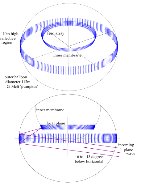
Figure 1: The physical geometry of the reflective outer section and the inner balloon feed array for the antenna modeling. Here we have modeled a SPB super-pressure balloon with about 29M cubic feet of volume and a equatorial radius of about 56m. The inner membrane has a radius of about 32 m.

EVA will deploy the largest-aperture physical telescope ever flown on a balloon payload, several thousand square meters, to be used to extend the radio-frequency collection power for neutrino impulses by a factor of 100 or more over any previous experiment. This will be accomplished using a portion of the physical balloon surface itself as the radio reflector, with a toroidal geometry as indicated in Fig.1, where an approximately 10 m high section of the balloon surface is covered with RF reflective layer, which need be only several skin depths thick, of order 10-20 $\mu$m at the wavelengths of interest. Although only a fraction of the physical area of the reflective region contributes to radio signal collection from any given direction, this area is still of order 100 square meters or more, equivalent to an 11 m diameter single-dish for 360 degrees of azimuth, and a usable range of 10-15 degrees in elevation angle.

Because we intend to operate at meter-scale wavelengths (from 0.5-2 m, or 600-150 MHz in frequency) where the Antarctic ice is nearly transparent, and galactic radio backgrounds are not an issue, and because we do not require diffraction-limited optics for mission success, we find that the balloon surface is quite acceptable as a focusing system. The location of the prime focus for the toroidal geometry is on an inner toroidal surface within the outer balloon. A planar-patch antenna array will be mounted on the surface of an inner balloon, with a grid spacing that will be optimized for cost-effective detection of the neutrino signals at a sensitivity that is at least an order of magnitude, and in the best case two orders of magnitude, better than any previous experiment. Triggering and data recording will be done on a conventional payload platform at the typical payload location at the base of the balloon system. Signals will be transferred to this package via analog optical fiber transceivers.

As we have noted above, EVA’s heritage is loosely based on the ANITA payload, the only prior experiment to search for UHE neutrinos via a long-duration balloon flight. ANITA currently has the best world neutrino limits in the EeV energy range ANITA2 . The strength of these limits derives from a key energy-dependent parameter of the detector: the effective acceptance of the neutrino aperture as a function of energy. Since we are concerned with an isotropic flux of neutrinos, it is the “all-sky” sensitivity that matters, and in ANITA’s case such sensitivity was achieved by an array of 40 horn antennas with angular response functions that each covered a patch of order 40 degrees in diameter. ANITA’s antennas were pointed at an angle of about 4 degrees below the horizon (the horizon is about 6 degrees below the horizontal at typical balloon float altitudes of $\sim 37$ km ) to maximize the volume of ice in their view, and their response thus extended to about 24 degrees below the horizon, covering more than 99% of the area in view. A combination of 4 or more antennas with overlapping response functions then determined a trigger when a radio impulse exceeded a pre-determined level above thermal noise.

For ANITA the neutrino acceptance was determined by how far out toward the horizon the system could trigger on a neutrino-generated radio impulse of a given radio intensity determined to first order by the neutrino energy. ANITA’s threshold for triggering on a radio signal was limited primarily only by the effective collecting area of the antennas involved. In practice, this effective area was of order 1 square meter. EVA will increase this effective area by a factor of 100 or more, and since the coherent Askaryan radiation total power increases as the square of shower energy, a factor of 100 increase in collecting area is required to get a factor of 10 improvement in neutrino energy threshold.

Energy Threshold & Sensitivity.

The sensitivity of a radio antenna and receiver is determined by its collecting area, the receiver’s bandwidth and integration time, and by the thermal noise background, which is the sum of the received thermal noise power from blackbody emission in the antenna field-of-view (also known as its “main beam”) and additive thermal noise from components such as amplifiers, cables, and filters that comprise the receiver system downstream of the antenna. The two contributions are often expressed as a sum of the antenna temperature $T_{ant}$ and the system temperature $T_{sys}$.

For a system designed to record only the impulsive events some type of threshold-crossing trigger is used to signal the presence of a signal peak in excess of background fluctuations due to thermal noise. The rms level of receiver voltage fluctuations in this thermal noise is given by

$$V_{rms}=\sqrt{k(T_{sys}+T_{ant})Z\Delta\nu}$$ (2.1)

where $k$ is Boltzmann’s constant, $Z$ is the receiver impedance, and $\Delta\nu$ the bandwidth. The antenna temperature is an average of the radiation temperature of all objects in the field of view, weighted by their apparent solid angle within the main beam (or main region of angular response) of the antenna. In EVA’s case $T_{ant}$ will be an average of the ice temperature, of order 230 K, and the sky temperature, which is several Kelvin at frequencies above 200 MHz. Noise figures of current off-the-shelf low-noise amplifiers are typically 90 K or less. Based on our ANITA experience with the Antarctic thermal noise environment, the root-mean-square receiver voltage for a 500 MHz band will be of order 10 microvolts, referenced to the LNA input, based on equation 2.1 above, using $T_{sys}\sim 300$ K.

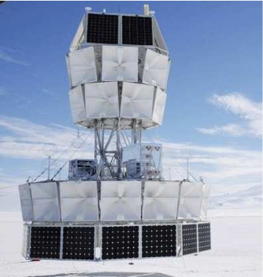
Figure 2: ANITA payload in flight-ready configuration.

Antenna effective area

ANITA’s quad-ridged horn antennas (seen in Fig. 2) determine to a large part the overall sensitivity, or its ability to “trigger” on RF impulses. These antennas had a boresight directivity gain of $10\log_{10}(G)\simeq 10$ dBi (dBi = decibels relative to an isotropic antenna), and it was roughly constant over ANITA’s frequency range of 0.2-1.2 GHz. Antenna effective collecting area $A_{eff}$ in terms of directivity gain $G$ and frequency $\nu$ is given by

$$A_{eff}=Gc^{2}/(4\pi\nu^{2})$$ (2.2)

where $c$ is the speed of light. Thus an antenna with constant gain vs. frequency has a collecting area which decreases as the square of increasing frequency. In practice, it was the off-boresight ANITA antenna gain at the typical adjacent-horn overlap angle for any given impulse that determines the average effective area for neutrino impulses, and this reduces the gain down to about 7 dBi . Since ANITA required a broad-band frequency content to trigger, the effective center-frequency at which to evaluate the average gain is about 400 MHz, and the implied effective area is 0.22 m² per antenna. In forming a trigger, the signals from 4 antennas that can view an incoming plane wave are used in a threshold-crossing square-law discriminator, but are not combined coherently, so the improvement in combinatorics goes as the square root of the number of combined antennas, and the net effective area for ANITA, in determining the radio sensitivity, is of order 0.5 m². This corresponds to an effective gain of $G_{eff}=4\pi A_{eff}/\lambda^{2}\simeq 11.2=10.5$ dBi.

This effective area sets the scale of the current state of the art for a balloon-based neutrino detector. For EVA our design requirement is to thus increase the effective area of the antenna by at least an order of magnitude, with a design goal of two orders of magnitude, a factor of 100. The implied minimum and desired gains, using again 400 MHz as the reference frequency, are

$$G_{min} = 112=20.5~{}{\rm dBi}$$

$$G_{goal} = 1120=30.5~{}{\rm dBi}$$

above an isotropic antenna. An estimate of the equivalent circular aperture dish diameter $D$ required to achieve this gain can be made by the approximation

$$D=\sqrt{\frac{\lambda^{2}G}{\pi}}$$

which indicates equivalent diameters of $D=4.5,~{}14$ m for these two cases.

Toroidal Balloon Reflector

Radio reflector antennas based on a toroidal geometry were first described by Kelleher and Hibbs in 1953 Kelleher53 , and Peeler and Archer in 1954 Peeler54 and summary analyses may be found in several modern antenna textbooks AE ; Wolff . The designs considered in prior work utilized a parabolic or elliptical curve rotated around an axis in its plane to form a surface of revolution. Although only those surface generated by rotating a circular arc actually conform to a true toroidal shape, all of these reflectors have been termed toroidal reflectors; we will follow this for convenience.

Here we choose the axis of rotation to be the vertical $z$-axis, and thus the reflective surface extends in the $\phi$, or azimuthal, direction. Obviously such surfaces of rotation must occupy only a portion of a full circle of rotation or incoming radiation would be blocked either fully or partially. Use of off-axis parabolic curves does not help in this case since the incoming rays are paraxial and thus, although the feed region does not occult the incoming wave, other portions of the reflector surface will, if they extend far enough around in azimuth. This constraint is acceptable for many designs involving toroidal reflectors, since they may still scan a wide range of azimuth, many tens of degrees or more.

However, in our case, the design goal is a system that can scan $360^{\circ}$ in azimuth, and a limited range of elevation angle , of order $10^{\circ}$. Use of a parabolic section for the surface of rotation would in this case give strong aberrations if used well off the main parabolic axis, so we consider a new configuration of the toroidal reflector with a near-circular generating curve, rotated around the $z$-axis to produce a complete toroid. Incoming plane waves enter below the reflective band, and are focused to a region above it. In our application, the incoming wave will be an RF impulse, and it will enter the toroid below the lower rim opposite to the active focusing area that will apply for that direction. Once reaching the opposite side, it is focused into an off-axis location with geometry that is locally an off-axis segment of a spheroidal mirror.

At the focal plane, a set of feed antennas, which are flexible planar patch antennas affixed to the surface of an inner balloon of appropriate size to approximately match the focal plane angle, receive the focused plane wave. The polyethylene surface and load tendon material of the balloon play no role in any of the wave propagation, as these materials are completely transparent and extremely thin on the scale of the wavelengths of interest here. The generating curve is determined by the average free-surface of the balloon, and such surfaces have been the subject of much detailed theoretical and experimental investigation Baginski1 ; Baginski2 . This design will retain spherical aberration, as noted previously, but such aberrations are generally more tolerable than the extremes of coma that develop in short-focal-ratio off-axis parabolic systems.

In practice a large scientific balloon requires vertical load tendons to support the total weight of the system, and these introduce a lobed structure for the balloon, leading to a scalloped surface. We will account for the scallops in our modeling of the surface, and they do constrain the highest radio frequency at which a balloon surface may be considered a coherent reflector.

Zero-pressure vs. Super-pressure balloons.

Stratospheric balloons have traditionally been constructed and filled such that they reach their full inflation at altitude at an equilibrium pressure equal to the ambient pressure at the float altitude, thus yielding a zero-pressure offset from the surrounding atmosphere. Vents on the base of the balloon help to ensure that any over-pressuring is avoided. Such balloons are known as Zero-Pressure Balloons (ZPB). The major drawback of ZPBs for our application is the fact that their shape can change dramatically depending on their thermal environment Baginski1 ; for example, in Antarctica in the austral summer, cooling of our ANITA-2 ZPB while over the very cold East Antarctic Ice Sheet caused a decrease of order 40% in the volume of that 29 Mcft ZPB, and a loss of altitude of 123,000 to 113,000 ft. In an Appendix, we provide a detailed description of the analytical basis for the two different balloon surface geometries.

After investigating to what degree we could tolerate such changes, we concluded that the preferable vehicle for our proposed application is a Super-Pressure Balloon (SPB) such as those that are now being developed for the NASA SPB Program Baginski1 ; Baginski2 . We note that the “pumpkin” shape of the current SPB design, with a ratio of the polar ($R_{p}$) to equatorial radius ($R_{e}$) of $R_{p}/R_{e}\simeq 0.6$, does give a larger astigmatism than a spherical design with more equal radii of curvature, and the physical optics of such systems would improve with a larger ratio $R_{p}/R_{e}$. But as we find in the next section, our initial investigations of such balloons as reflector systems is very promising.

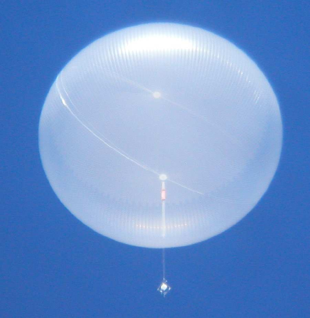
Figure 3: Flight 591NT SPB at float altitude during the 2009 flight.

Analytical design guides.

To select an initial geometry for the reflective section of the balloon for numerical modeling purposes, we refer to results derived for toroidal reflectors with parabolic generating curves as a guide. Adapting these results for a spherical generating curve, the path difference function for any location on the reflector surface can be approximated analytically with first-order accuracy, following Wolff (1966) Wolff as

$$\Delta=-2\hat{f}\left[1-\frac{\cos\phi^{\prime}(2-\zeta-\cos{\phi^{\prime}}+\hat{f}\cos\phi^{\prime}}{1+\hat{f}-\zeta}\right]$$ (2.3)

where $\hat{f}$ is the effective focal length normalized to a unit equatorial radius for the balloon (for spherical surfaces the physical focal length $f\sim R/2$); $\phi^{\prime}$ is the azimuthal angle of the location of the reflection point relative to the direction of the incoming plane wave, $\zeta=\sqrt{1-z^{2}}$, and $z$ is the vertical coordinate, normalized to the equatorial radius.

To simplify the numerical modeling requirements, we wish to simulate only an azimuthal subregion of the total toroidal band, where the azimuth we are considering in this case is not the azimuth of an incoming plane wave, but that of the toroid as viewed from the center of the balloon. The overall reflection geometry ensures that the azimuthal width of the appropriate subregion is well under $\pm 90^{\circ}$ around the optical axis, but to refine this we use the analytic results to determine an acceptable subregion. A family of curves, showing the path difference for reflected rays at slices of equal elevation derived from this equation is shown in Fig. 4, where in this case $\hat{f}=0.46$ and the radius of the balloon here is 56 m. It is evident that at distances off the equatorial plane, the phase error, while improving at higher $z$ at low azimuth angles, rapidly degrades at higher azimuth angles. Using the Rayleigh quarter-wave criterion as a guide, it is evident that the azimuth region over which the phase difference is acceptable extends to about $\pm 30^{\circ}$ for a reflective band of order 20 m high, giving of order 1000 m² of usable coherent surface area in the ideal case. In practice we will restrict the simulation to smaller subregions of the reflector, because of other constraints such as the clear aperture for incoming plane waves, but these results provide good overall guidance for developing the models.

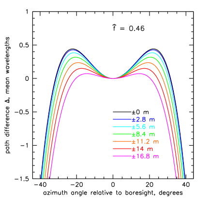
Figure 4: Path difference of toroidal reflector for a normalized focal distance of $\hat{f}=0.46$, for various slices of elevation above the horizontal mid-plane of the balloon.

These results also apply only to on-axis plane-waves, and our design will also require focusing of rays that are well off-axis. Recent results in analyzing parabolic toroidal reflectors have validated elevation scanning ranges of $>7^{\circ}$ Chu89 with less than 1 dB reduction in gain, and azimuthal ranges for toroidal reflectors have been used effectively out to the $\pm 30^{\circ}$ suggested here, or even more. For purposes of our investigation, we consider initially a reflective band of 11 m total height, and about 50 m width, corresponding to an azimuthal range of $\pm 25^{\circ}$ for a 56 m radius balloon.

As we will see below, the standard balloon surface has a factor-of-two different radii of curvature in the circumferential and meridional directions, and this will have important impact on the behavior of the surface as a focusing system. Such a surface is too complex to easily quantify within the analytic framework, here but it provides us with a starting design which we will evaluate numerically below.

A photograph of the fully inflated 7 Mcft superpressure balloon used in the successful 54 day flight 591NT can be seen in Fig. 3. In early 2011, a successful Antarctic flight of a 14Mcft design was completed (flight 616NT Cathey2011 ), verifying the scaling criteria used to develop this next step in the program. To date, the most difficult problem associated with each step in scaling up the SPB designs has been the deployment of the balloon as it inflates. In earlier designs, lobes would often remain folded over one another even in a fully inflated balloon, leading to distortion and unplanned stress in the balloon surface. However, in the most recent designs, this problem appears to have been solved through a new analytic method Baginski3 , and all recent SPB launches have deployed successfully.

II.2.1 SPB shape stability

Although SPB shapes are clearly far more stable than ZPB shapes, there are still variations in the differential pressure of the inflated balloon that could lead to changes in the focal properties of the surface. Typical mean differential overpressure for the SPB tests to date are about 50-60 Pa, and variations of $\pm 30-40$% have been observed due to variations in the solar angle and float environment. Baginski & Brakke Baginski3 considered the strained shape of the gore for the Flight 591-NT design, which also formed the basis for the 616NT designs as well. Let H be the height of the balloon (measured from nadir fitting to apex fitting) and D to be the diameter. They found $H=50.32$ m and $D=82.11$ m when the nadir differential pressure $P_{0}=120$ Pa. In Table 1, below we present the dimensions when $P_{0}$ is between 19.9 and 120 Pa; $H$ and $D$ were not reported in Baginski3 .

Table 1: Super-pressure balloon height and diameter as a function of differential balloon pressure, as found in Baginski3 , for flight 591NT.

$P_{0}$ (Pa)	$H$(m)	$D$(m)
120.500	50.325	82.115
99.256	50.326	82.021
77.991	50.355	81.920
56.867	50.444	81.804
36.522	50.674	81.654
19.902	51.248	81.416

For the actual flight, pressure gauges indicated that $P_{0}$ varied between a minimum of 30 Pa (night) and a maximum of 75 Pa (day) (see Cathey ). From the third and sixth entries in Table 1, we find $\triangle D=0.5$ m and $|\triangle H|=0.9$ m. Similar variations were seen for the 14 Mcft balloon in flight 616NT Cathey2011 . Our analysis indicates that such changes will lead to focal effects that are well within the depth-of-focus tolerance ranges we have found both in simulation and our scale-model tests, as we report below.

In addition to pressure-induced shape changes, any pendulum motions of the balloon could also have an impact on the stability of the field-of-view of the reflector surface. Fortunately, pendulum motion of stratospheric balloons at float has been measured for many different flights. Apart from a period of a few hours once the balloon reaches its float altitude, pendulum-induced tilts in the balloon are very small, a small fraction of a degree typically.

NEC2 Modeling.

As a proof-of-concept we have created a detailed antenna model for a geometry involving a 29 Mcft SPB balloon with approximately 56 m radius, and this model is the basis for several of the figures provided here. This balloon size presents a significant advance in the current scale of these balloons, but is a standard ZPB size, and there appear to be no technological limitations to scaling up the current SPB designs to this level. However, we note that after development of this model and the analysis described here, the SPB program adopted a goal of a 25 Mcft design for future use, and our scale models currently built and planned will all conform to this design.

Antenna modeling is done with the Numerical Electromagnetics Code version 2 (NEC2) NEC2 , a method-of-moments full-electromagnetic solver based primarily on wire-frame modeling of conductive structures. It has the virtue of allowing straightforward wire-frame model prototypes to be built up into fairly complex structures, which can produce realistic results even for surface modeling, although they will underestimate reflectivity of continuous conductor surfaces because of the wire grid approximation. Although NEC2 can also use facet patch segments to create filled surfaces, this capability of the code is much harder to accurately utilize, and thus we have made use of only wire-grid models here.

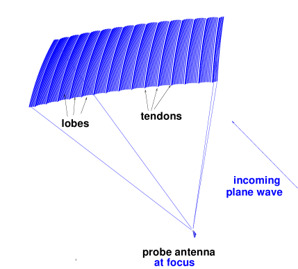
Figure 5: NEC2 model geometry used for gain estimation.

A detail of the model is shown in Fig. 5. In practice the NEC2 models which use the entire array are prohibitively large for calculations, and as we have noted above, we thus restrict the modeling to a subregion of the reflector approximately $\pm 25$ degrees wide in azimuth and 11 m high; these choices were deemed conservative given the additional constraints we have that go beyond the analytic model. This section is shown in the Figure, along with the location of the wideband probe antenna which is used to excite the structure in the NEC2 model. All of the modeling was done using the reciprocity relations for antennas, which ensure that transmitted-wave response functions may be used to estimate the received-wave response functions.

We model the surface as having two radii of curvature: the circumferential, or “hoop” radius $R_{h}$, and the meridional radius of curvature $R_{m}$. the relation $R_{h}=2R_{m}$ is generally true for pumpkin balloons due to the intrinsic shape of the Euler-elastica, which is the analytically derived curve for such surfaces.

There are thus two primary aberrations involved in the image formation of these reflector segments: (1) Spherical Aberration, which causes central rays near the optic axis to focus further away than the marginal rays on the outer edges of the reflector; and (2) Astigmatism, which causes a different focal length for the two different radii of curvature.

In addition to these primary aberrations, we have also accounted for a secondary aberration which is important to balloon surfaces: the tendon-gore structure of balloon fabrication leads to a scalloped surface where the tendons have a smaller radius than the center of the gore, and lobes form in the surface. In addition to the primary radii of curvature $R_{m}$ and $R_{h}$, the individual pumpkin lobes have a bulge radius of $r_{b}$, typically several meters, as described in the Appendix.

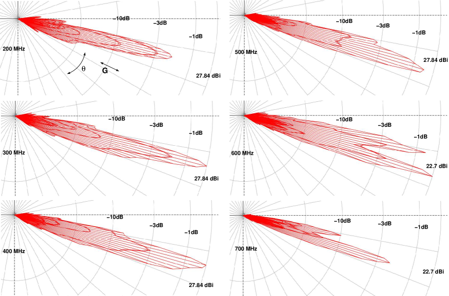
Figure 6: Elevation gain polar plots for six frequencies and the largest off-axis elevation angle (about -13 degrees) expected to be observed with EVA. The gain peaks at about 27.8 dBi, exceeding the design goal of 26.9 dBi indicated previously. Note the gain scale change in the two highest frequencies.

For our simulated balloon we have assumed about 300 total gores, several of which are evident in Fig. 5. We have assumed a typical case where the fully-inflated lobe center is about 10 cm further out than a line joining the tendons. This value is about 20% of the wavelength at 600 MHz which is currently the upper end of our design frequency.

II.2.2 Model results.

The model NEC2 analysis was done by iterative optimization of the gain vs. frequency and angle for different locations of a probe antenna which acted as the feed excitation for the larger toroidal section. Starting values for the best feed location were based on the sagittal and transverse foci of the astigmatic reflector. We found that the best gain values and apparent circle of least confusion for the focused antenna beam tended to favor that equatorial radius of curvature, primarily because there was more reflective area available at the larger focal distance, and the depth of focus was also larger. We did not adjust the width of the vertical reflective section; this is another parameter that could be optimized. Our NEC2 model filled the aperture of the reflector with the equivalent of 10 cm diameter “wires” at a spacing of about 35 cm, corresponding naively to about 30% reflectivity of the surface; this value was chosen as the closest that we could place the elements while still maintaining robust numerical stability for the calculation. Thus the estimated antenna gains should show some improvement with fully-filled reflective sections.

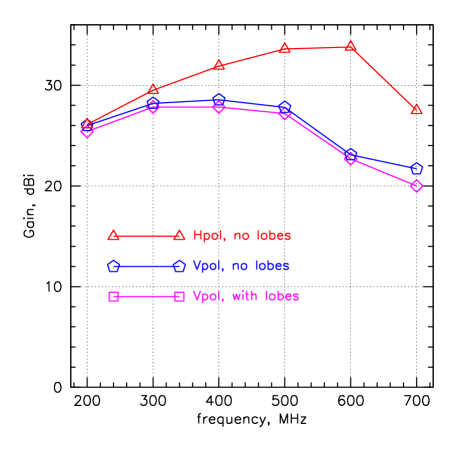
Figure 7: Peak gain vs. frequency for the models described in the text, including vertical polarization with and without the lobe-tendon structure of the surface, and horizontal polarization, also with a smooth surface here.

Fig. 6 shows the primary results of the simulation: polar plots of the antenna absolute directivity gain vs. elevation angle for the largest off-axis elevation angles of interest for EVA. The toroidal antenna is designed to observe the angular range from a few degrees above the geoidal horizon (which is about 6.8 degrees below horizontal for our suborbital altitude) to an angle of about 8 degrees below the horizon, a range which covers 96% of the Earth’s surface area in view in the lower hemisphere. Event plane-waves that arrive from steeper upcoming angles are reflected progressively further off the optic axis, and are thus subject to more sever aberrations. The results shown here are for the one of the steeper angles of interest, $13^{\circ}$ below the horizontal. We have also confirmed that the shallower angles corresponding to events near the horizon do give better results and slightly higher gain.

The plots show a wireframe structure of the gain values, where elevation is sampled in 1 degree increments. Azimuth angle structure can be derived also from this plot by noting the location of the transverse wire frame contours of the azimuth sampling, which was done here in 0.5 degree increments . The plots cover the range from 200-700 MHz, and the gain over this range has a broad plateau of 26-28 dBi from 200-500 MHz, and then drops to 22.7 and 20.4 dBi respectively at 600 and 700 MHz.

Clearly the image formation is seriously degraded at 600 MHz and above, with a double-lobed structure appearing in simulation at 600 MHz. It is evident that the optical aberration at these higher frequencies has grown to the point where partial destructive interference is taking place in the image-forming region. In any case, our results do indicate that over the frequency range from at least 200-500 MHz (a fractional bandwidth of order 1) the net directivity gain of the system approaches within a factor of two of the design goal, and already well above the minimum requirements. The antenna thus achieves a broadband response that is suprisingly good given that the surface shape is not controlled in any way.

We have not yet attempted to further quantify the cause of the high-frequency aberrations, nor have we done any optimization of the system to improve the higher frequency response. We do note that it is relatively straightforward to include a circumferential reflective membrane just within the outer inflation surface, which can reduce the large difference between meridional and hoop curvature, as well as minimizing the effects of the lobes. While we have not analyzed such a band in the current work, the potential for improvement in bandwidth and gain could offset the additional complexity of construction and deployment.

Variations: horizontal polarization, and suppressed lobe structure.

The simulation results shown here are for the vertical polarization with the lobe and tendon structure included in the model, as noted above. We have also investigated the behavior of the model with the lobe and tendon scalloping suppressed, as would be the case for a balloon with reflective film that spanned the intergore regions. Such interior membrane structures have also been mechanically modeled for their dynamics on the balloon surface, and they appear to be benign in their behavior, with respect to the balloon inflation and operation. In addition to this secondary model for vertical polarization, we also developed a similar wireframe model for horizontal polarization to ensure that there were no adverse effects in detecting a wide range of polarization planes.

We found that the lobe and tendon structure of the balloon surface has very modest effects on the antenna gain, as shown in Fig. 7, which plots the resulting gains vs. frequency for the three configurations described here. We also found that the double-peak structure at 600 MHz was present for vertical polarization even in the smooth-surface case, indicating that the effect is likely due to the large scale aberrations rather than the surface relief induced by the lobe structure. Given that the dual gain peaks seen at 600 MHz are not centered on the gain peak at lower frequencies, there is likely to be some destructive interference at that frequency which is suppressing the main peak in favor of nearby sidelobes; there are techniques that can remediate these effects, such as tapering of the reflectivity at the top and bottom of the reflective band.

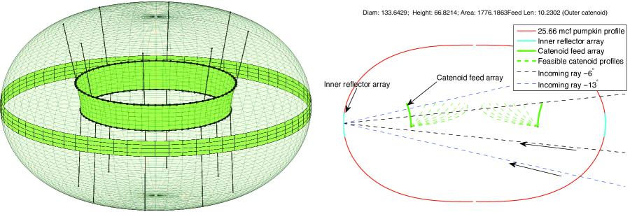
Figure 8: Left: 3D model of a 25.66 Mcft superpressure balloon with a possible catenoidal surface shown schematically as a location for the feed array. Right: cross section of the balloon surface and catenoid, showing the range of sections that are possible, and ray paths for the modeled sections.

Of equal interest is the fact that the horizontal polarization results show no similar effects at 600 MHz, in fact we found that the gain curve retains a single peak throughout this frequency range, and that the overall gain is several dB higher, probably because of the lack of edge effects for the E-plane of the field which is now aligned with the longer portion of the reflector. In any case, the horizontal polarization performance exceeds that of the vertical polarization, and well exceeds the requirements for total gain.

II.2.3 Smaller SPB designs.

All of the modeling done here for a balloon of 56 m radius can be applied to a smaller radius superpressure pumpkin with appropriate scaling. For example we also investigated the 14.8 Mcft, 46 m radius SPB design, which was recently flown in the 22-day NASA SPB flight 616NT Cathey2011 . Under these conditions we find that similar beam-pattern results are obtained if we scale the equatorial reflector region height from 10 m down to 8.2 m. The expected gain in the mid-frequency region at 300-400 MHz scales as $(D/\lambda)^{2}$ and we thus anticipate a decrease of about 2 dB in overall gain, still preserving the possibility that a smaller balloon may be able to achieve the science goals for EVA, although the smaller free-lift capacity would levy restrictions on the payload mass budget.

II.2.4 Feed array system.

The feed array system is currently envisioned to occupy an interior band around the surface of an inner membrane. Lacking detailed knowledge of the shape of the focal plane surface, we anticipate that the inner membrane could either be over-pressured for a convex focal surface, or it may be developed as a catenoid surface if a concave focal plane is necessary. Currently our antenna modeling does not give sufficient information to clearly delineate the focal surface structure; this will be determined as part of the study we propose here. If the membrane is over-pressured in an upper chamber to produce a convex surface, the design may be accommodated with a membrane having cylindrical symmetry, fused to the upper surface, and possibly tensioned to the central collar at the base of the balloon. If, as appears more likely in our current models, the region of best-focus is in fact concave, we have explored catenoid surfaces with a partial membrane containing the feed array, as shown in Fig. 8.

Each feed antenna will be a low-gain planar patch antenna, probably with dipole-like response. Normal radio astronomical systems require that a feed antenna have a directivity that fills only its main reflector, thus a fairly high gain (6-10 dBi) feed antenna may be required. In our case, since the antenna temperature of the main reflector will be dominated by the 240 K temperature of the ice in its view, the feed antennas need not be directed only at the main reflector aperture, as any “spillover” in this case will be into either cold sky or ice. Also it is important to note that our feed antennas are not used as transmitters; a transmitter feed must not waste power into directions other than its main reflector, but for a receiving system, this consideration is irrelevant.

For the focal length of our NEC2 model, which was of order $f=25$ m, the focal plane transverse scale is given to first order as $f^{-1}=0.04$ radians/m, or about $2.5^{\circ}$ per meter. We need to sample over an elevation range of about 8 degrees, or just over 3 m wide. The broadband feed antennas are expected to be of order $\lambda/2$ at the longest wavelength of interest, thus we expect about five antennas along the elevation scan direction. From the gain plots above it is evident that the full-width-half-maximum of our elevation beam is about $3-5^{\circ}$ in elevation, and about $0.5-1.5^{\circ}$ in azimuth. Thus we anticipate oversampling in elevation, which will allow for multi-antenna triggering as was used in ANITA, as well as phase-gradient measurements to refine the elevation angle measurements of any event. Azimuth sampling will be matched to first order, giving angular resolution of $1-2^{\circ}$ in azimuth, which has proven to be adequate for ANITA. We anticipate a total of 1200 patch antennas to cover the required solid angle.

III Results of microwave scale-model tests.

We have constructed a microwave scale model testbed for exploring the behavior of sections of a toroidal surface, including the effects of the balloon gores and tendons. This has been accomplished by computer- numerically-controlled machining of exact 1/35 and 1/26 scale models of a computer generated model for the fully-deployed surface of a 25 Mcft super-pressure balloon, following the current planning design adopted by NASA for their SPB program. We have also developed several different microwave receiver antennas, including a prototype patch array. A photograph of one of the test setups using the 1/35-scale model, taken in an anechoic chamber is shown in Fig. 9(Left). The scale model was illuminated with a 1.8 m wide collimated microwave beam made by a large off-axis paraboloidal reflector, situated opposite the EVA test stand. Because of constrants of the scale model machining, we restricted the width of the reflective section to a smaller region than was simulated in our NEC2 models; the scale model corresponds to a $\pm 15^{\circ}$-wide azimuthal section of the balloon rather than the $\pm 25^{\circ}$ section that we simulated. As a result we anticipated that we might observe somewhat lower total gain for the model vs. the simulation.

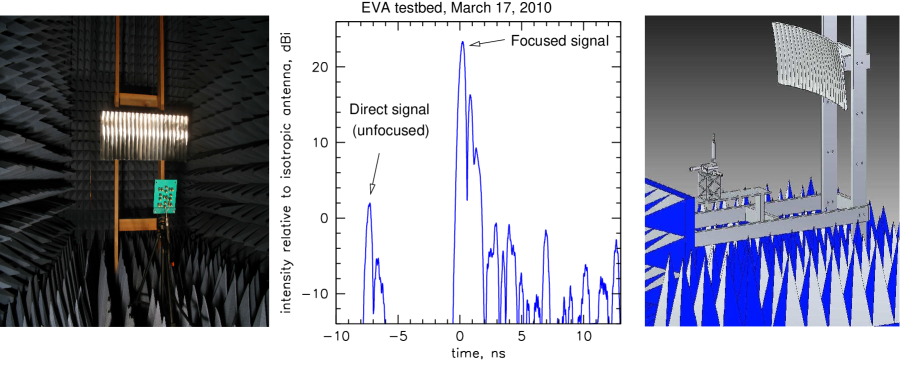
Figure 9: Left: Photograph of 1/35 scale model of toroidal balloon section, equivalent to a 10 m high, by 30 m wide section of the full balloon. Center: initial results of the focusing test with the toroidal scale model, using a microwave pulse in the 6 GHz range (200-300 MHz equivalent scaled frequency for the 1/26-scale model). The pulse to the left measures the unfocused incoming plane wave intensity using a patch dipole antenna, the much larger peak at center is the focused response with a peak directivity gain of 23.4 dBi. Right: diagram of the test setup with the 1/26-scale model, including a micrometer stage at the focal region used to profile the focused beam parameters.

Our initial impulse testing using the 1/35th scale model was challenging due to frequency limitations imposed by our test equipment, and we could not accurately test the system above an equivalent reference frequency of about 150 MHz. In our initial testing of this system, which was also limited by our current coarse positioning system, we measured a directivity gain of order 16 dBi. Using what we learned from this model, we then constructed the larger 1/25-scale model, again with near-perfect fidelity to the simulated balloon surface, as afforded by the CNC system. We retained the lobes and tendons in our model to maintain a conservative approach, although it appears sxtraightforward to suppress the effects of this structure in practice using internal reflective films that span the lobes.

With this new model, we have now measured a directivity gain factor in vertical polarization of up to $G=220$ relative to an isotropic antenna, or in equivalent terms, 23.4 dBi, at a microwave frequency of about 6.6 GHz, corresponding to 260 MHz for the full-scale. This value is within about 3 dB of the NEC2 model prediction, and already well above our minimum performance requirement. Fig. 9 (left) shows a photograph of one of the initial test setups, with a prototype patch array at the focal plane. The middle pane of the same figure shows the layout of a micrometer stage now in initial testing for higher-precision focal plane measurements. To the right are the data validating the performance noted above. The smaller peak to the left is the incoming plane wave impulse signal detected by the backlobe of the patch as it passes by before focusing, then the much larger signal (here in logarithmic units of intensity) arrives from the balloon reflector section. Due to constraints imposed by our transmitting system, we have only been able to investigate vertically polarized signals to date, though based on our simulation results, we expect that the horizontal polarization results will likely exceed the vertically polarized results in their performance.

It is evident that these results already validate the basic premise of EVA: that a toroidal reflective section on an unmodified super-pressure balloon surface already possesses quite compelling optics for radio astrophysics applications such as we envision.

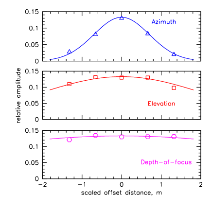
Figure 10: Three-dimensional focal region measurements (points) of the response function of the EVA model, with fitted Gaussian beam curves shown. The dimensions have been scaled to the full size of the reference balloon model.

Another important issue in EVA performance is the shape of the focused beam, including the depth of focus, and the width and height of the main lobe of the beam in the focal plane. This has important implications for the control fidelity of the membrane surface and for the metrology precision. We have made preliminary measurements of the beam shape over the principal axes on the 1/25th scale model. These measurements were made using the micrometer system depicted in Fig. 9 (right), and the results are plotted in Fig. 10, with the measurements (points) fitted to Gaussian beam parameters (curves).

We find that the beam is narrowest along its transverse dimension (eg, projected azimuth), with a Full-Width at Half-Maximum (FWHM) of 1.14 m scaled equivalent. Along the direction of the beam, our micrometer translation was not adequate to find the half-power points, and the resulting lower limit on the depth-of-focus is $>3$ m. Transverse to the beam in the vertical (eg. elevation) direction, we find again a very broad maximum with FWHM $\sim 3-4$ m. These values are consistent with our modeling expectations, and provide us with clear design direction for both the sampling density of the focal plane patch antenna array, and for the level of control that will be necessary for the inner membrane in order to retain good focal plane response.

IV Other EVA Subsystems

IV.1 Receivers.

The RF front end for EVA will consist of an integral front-end bandpass filter followed by a low-noise-amplifier (LNA)/power limiter combination, with about 36 dB of gain, and a second stage amplifier designed to boost the signal up to the point where an analog optical driver can modulate it onto optical fiber, an additional 20 dB or so. These elements are all in close proximity to the patch antennas to ensure no transfer losses through cables, and are enclosed in a flexible Faraday pouch for additional EMI immunity. The signals from the LNA then drive an analog fiber-optic radio-frequency link, and are transmitted via single-mode fiber along the inner balloon tendons, and led down through the base collar to the flight train and eventually to the payload at the bottom. The power budget for the single-patch LNA+2nd-stage amp+fiber transceiver is 0.8W per channel for 1200 patch antennas, and these are fed from the 1.2 kW photovoltaic array at the outer balloon-top platform (BTP). The expected noise performance of the LNA and bandpass filter combination is about 90 K on average per channel, and we have already demonstrated this performance in the ANITA-2 flight.

IV.1.1 RF Interference

The three completed flights of ANITA (and its prototype ANITA-lite) have also provided excellent information regarding the anthropogenic noise environment in Antarctica, and strategies for managing the receiver and trigger systems in the presence of such noise ANITA-inst . ANITA has demonstrated that, apart from regions close to the major bases – McMurdo Station, South Pole Station, and a few others – the anthropogenic noise is sporadic and does not add significantly to the thermal noise environment, nor does it saturate the trigger systems of instruments such as ANITA and EVA. Clearly the higher sensitivity of EVA will lead to a higher trigger rate on weak RFI, but such triggers can be rejected in real time by their association with known bases or camps.

IV.2 Analog fiber-optic transceivers.

Transmission of the data from the antenna feeds to the instrument payload cannot be done via coaxial cable due to weight concerns, therefore, RF over fiber technology will be used to convert RF to optically modulated signal over single-mode fiber optic cable and back to RF at the payload using a custom-built fiber interface using commercially available laser diodes and PIN photodiode receivers.

The concept of using optical fiber to connect antennas at a distance to the signal processing equipment (”antenna remoting”) has been actively studied by industry for WLAN distribution Yakoob ; Ackerman as well as several other scientific collaborations. Most recently, the Australian Square Kilometer Array Pathfinder project conducted experiments using a commercially available ($30 in quantity) vertical cavity surface-emitting laser (VCSEL) and demonstrated the feasibility of connecting 7200 antenna feeds using directly-modulated VCSELs Beresford . Improvements in high-efficiency VCSELs Furukawa should reduce the noise figure to a tractable level. The primary power cost of the VCSEL transmitter would be in the RF amplification needed to compensate for the noise figure of the optical link, with a target of less than 0.5 W/channel – about a factor of four below typical powers in current commercial devices.

IV.3 Trigger/Digitizer System.

We anticipate utilizing a trigger system closely based on ANITA heritage. The incoming RF signal, once it has been extracted from the optical receivers, is split conceptually into two paths, one of which is used for triggering and the other for digitization of the waveform if a trigger is detected. Because we are using a factor of 15 more signals that ANITA, we will effectively implement a decimation scheme for digitizing the data, so that a trigger does not require digitization of large portions of the feed array.

Improvements in the ASIC technology for low-power waveform samplers have enabled deeper storage and demonstrated concurrent read/write operation BLAB1 . Incorporation of a discriminator has also been shown to be feasible, and this allows for the concurrent function of both trigger and sampling in a single ASIC. Thus while we still maintain the conceptual difference of the triggering vs. digitization paths in our system, in practice, the functions will be effectively co-located for EVA.

We have adopted the following preliminary specifications as a working architecture for EVA. Optical signals arriving from the main E/O fiber bundle are broken into groups of 32 signals each that go into approximately forty compact Sampling Trigger Modules (STMs) which each contain Application Specific Integrated Circuits (ASICs) based on a next-generation version of our current LABRADOR chip LAB . These ASICs are designed to handle internally both triggering and sampling via a switched-capacitor array. Digitization only proceeds upon external command.

Local STM trigger signals are broadcast to a central DAQ module in the system. This trigger master than analyzes these trigger primitives and broadcasts feed-array region-specific readout window requests to the STMs at up to approximately a 1kHz rate. Samples in these selection windows are then digitized and sent back to the DAQ crate.

Each STM has bi-directional trigger and data high-speed links to the central DAQ which may utilize digital 1.2 Gbps or greater fiber optic transceivers for noise immunity and speed. The STM consists of 4 trigger/readout ASICs and an FPGA. This FPGA handles the serial transmission using the Xilinx Aurora protocol or similar. Each of the 4 ASICs has 8 channels of input, and provides 8 Low-Voltage-Differential-Signal (LVDS) trigger outputs corresponding to internal 1-shots that discriminate the full-RF-band trigger. Carrier wave rejection in the trigger will be performed using directional trigger masking.

Local pattern triggers among the feed-array signals are formed in the FPGA, and broadcast via phase-offset encoding over the digital fiber link. Global triggers are formed in the DAQ master crate and broadcast over the DAQ fiber uplink, resulting in a digitization command. The Trigger high-speed link is used for clock, timing and commanding.

The digital data requested in response to a central DAQ module trigger decision could arrive at the rate of up to 40 kHz, and must then be further decimated since this rate is completely dominated by incoherent thermal noise fluctuations rather than coherent plane-wave impulses. A dedicated co-processor (which may just be a specific core or pair of cores in a multi-core host processor) will make on-the-fly reconstruction approximations to the digital waveform data and determine which signals are consistent with coherent impulses to first order. We expect to write data to the solid-state storage system at no faster than about 50Hz, and this rate will still be dominated by thermal noise, but will provide a continuous measure of instrument health. Event size is estimated at about 40 kbyte per event compressed, and this will yield about 9TB of data in a 50 day flight.

IV.4 Metrology system.

EVA’s precursor mission ANITA had a mission critical requirement for moderate accuracy orientation measurements, to ensure that the free-rotation of the payload would not preclude reconstruction of directions for events at the degree level of accuracy. Such measurements were accomplished with a redundant system of 4 sun-sensors, a magnetometer, and a differential GPS attitude measurement system (Thales Navigation ADU5). These systems performed well in flight and met the mission design goals. In calibration done just prior to ANITA’s 2006 launch, we measured a total $(\Delta\phi)_{RMS}=0.071^{\circ}$, very close to the limit of the ADU5 sensor specification, and well within our allocated error budget.

For EVA, the issue of measuring the absolute orientation has shifted from the payload position in the flight train to the balloon itself, along with the inner feed membrane. To accomplish a measure of the orientation and attitude of this system, we will use a separate metrology system to locate fiducials married to the surfaces of the outer balloon and inner membranes at strategic locations. For orientation and attitude to be accurately measured from the inner surfaces, including the reflector and feed array, we anticipate a need for several-cm-level precision. We have demonstrated such precision already using photogrammetry for the ANITA payload; implementation of this for EVA will require periodic digital imaging of the balloon system from the BTP, with particular attention to the fiducials. Laser or microwave ranging systems may also have the capabilities necessary to augment or replace our photogrammetry approach.

Timekeeping.

Payload timekeeping for EVA will be required at several different levels. Dual GPS units will be used for absolute synchronization with UT at the 50-100 ns level. One of these units also will be used to discipline the onboard computer clock, for millisecond-level time tagging of events. A separate counter keeps track of nanosecond-level timing between digitizer boards and can link events at longer time scales (of order 1 sec) as well. These systems are based on successful systems used for both ANITA flights, and contain various levels of redundancy which served ANITA well during both of its flights.

V Technical Challenges: Construction & Launch.

EVA presents challenging issues of construction and launching of the balloon and feed membrane system. We have reviewed these issues with NASA Columbia Scientific Balloon Facility engineers CSBF1 . The innovations associated with the EVA design all represent extensions of technologies and methodologies that have one or more precursors in existing balloon experience. For example, reflective radar tape is used for many balloons that are launched in regions where aircraft activity may be present to ensure that the radar cross section is suitably large. Balloon-cap packages, while not common, are a relatively accepted method of extending payload functionality when necessary. Inner membranes have been utilized in the past for a few discrete investigations, although none with the complexity of the EVA membrane. However, this program will clearly require the development of new production and assembly methods at the manufacturer of the balloon (AeroStar International is the current NASA-sponsored contractor for this), as well as new launch methods and associated hardware at CSBF.

VI EVA predictions for rates

VI.1 UHE Neutrinos.

Table 2: Expected numbers of events from a full range of BZ neutrino models for a 50-day EVA flight compared to the combined sensitivity of ANITA-I and ANITA-II, which had a net 45 days of livetime. The last column gives the range of improvements in the event totals.

BZ neutrino models	Events,	Events,	ratio,
	ANITA-II,28d	EVA,50d	EVA/ANITA
Mixed UHECR composition Auger07a	0.05	5.0	100
Minimal, no evolution  Engel01 ; PJ96 ; Aramo05	0.3-0.9	9.2-38	$\sim 40$
$\Omega_{m}=0.3,\Omega_{\Lambda}=0.7$, Standard model Engel01	0.7	29	41
Waxman-Bahcall $E^{-2}$ flux (minimal) WB	0.49	6.5	13
GRB UHECR-sources Yuksel07	1.44	66	46
Strong source $z$-evolution Engel01 ; Aramo05 ; Kal02	2.2-5.3	40-60	11-18
Maximal, saturate all bounds Kal02 ; Aramo05	16-25	180-220	$\sim 10$

Using the results from our antenna simulation, and the basic triggering scheme outlined above, we have developed a Monte Carlo event simulation code to investigate whether, using the frequency-dependent NEC2 model antenna gains described above, EVA could achieve its minimum mission goal of achieving at least one order of magnitude improvement in neutrino flux sensitivity, with a desirable goal of two orders of magnitude improvement. Since ANITA now has the best limits in our energy range, we use the ANITA flux estimates as our baseline for comparison. We estimated effective neutrino apertures and event rates for a 50-day flight, such as achieved by SPB flight 591NT.

Table 2 presents the results of this simulation in terms of the comparison of total neutrino events detected for a range of different models. For these results, the energy threshold for EVA was improved by roughly and order of magnitude compared to ANITA, giving the majority of triggered neutrino events in the energy range from 0.3-3 EeV. Our results indicate that EVA can improve current limits factors of 10-100 in total events detected, depending on the BZ neutrino model used. The lowest flux model, in the first line of the table, presents a very difficult detection problem, and is based on a mixed-UHECR composition as suggested by the Auger Observatory recent data Auger07a . EVA is able to reach this challenging model, and all others that are current in the literature. In the last line of the table, the models are in fact already ruled out by ANITA results ANITA2 , but we include this line for completeness.

VI.2 UHE Cosmic Rays.

One of the most interesting results of the ANITA flights has been the serendipitous observation of 16 or more ultra-high energy cosmic ray events, observed mostly in reflection off the ice sheets, with their impulsive radio emission arising via the geosynchrotron process in the Earth’s magnetic field ANITA_UHECR . Due to the largely vertical geomagnetic field in Antarctica, these events appear with nearly pure horizontal polarization, and are thus cleanly separable from the neutrino events, which are dominated by vertical polarization due to the Fresnel geometry for refraction out from the ice to the balloon payload.

These events, whose mean energy approaches the GZK cutoff energy, signal a new methodology for probing the UHECR spectrum near the endpoint, which may be able to effectively complement ground-based techniques. ANITA-III, due to fly in the 2013 season, and that will have a trigger that is optimized for both UHE neutrino and UHECR detection, is expected to observe several hundred such events, including of order 60 events above the UHE energy at $10^{19}$ eV, and a handful at or above the GZK cutoff energy at around $3\times 10^{19}$ eV.

Super-GZK events, those with energies above $10^{20}$ eV, are a challenge for any ground-based observatory; in nearly 5 years’ of observations, the Auger observatory has seen only of order 3 such events, and ANITA-III, despite the significant increase over prior flights, still does not effectively probe the super-GZK range. EVA, with much higher potential sensitivity than ANITA, may be expected to observe a much larger sample of UHECR events, and we have simulated its potential sensitivity for UHECR detection, using simulations developed for and validated by ANITA’s UHECR analysis. We have also confirmed that ANITA experimental measurements still do not agree well with any of the current ground-based simulations, and thus we have used the experimental field strength estimates determined by ANITA for our EVA simulation as well. Changes in the results are likely to appear primarily in the energy scale rather than the total number of detected events, since that is the largest uncertainty in the ANITA field-strength estimators.

We find that EVA’s total rate of detection of cosmic-ray-generated radio events will be a factor of 20 higher than that predicted for ANITA-III, with of order $15,000$ events detected in a 50-day flight, a rate of 300 per day, compared to about 15 per day expected for ANITA-III ANITA_UHECR . The vast majority of these events arise from relatively nearby lower-energy cosmic-rays, with a mean energy of several EeV. Of order 500 of the sample have energies exceeding $10^{19}$ eV, and of these, 60 or so are in the GZK cutoff range above $3\times 10^{19}$ eV. Only one or two events above $10^{20}$ eV may be expected due to the fact that, despite the very large area – of order $10^{6}$ km² – observed by EVA, the small solid angle for detection of the highly-beamed geosynchrotron radio emission leads to an effective saturation of the acceptance at high energies. We expect to have initial energy resolution comparable to that estimated for ANITA: $\Delta E/E\sim 50-100\%$. However, the much larger event sample will provide statistics in the region of the GZK cutoff (the only clear feature in an otherwise smooth power-law distribution) that will enable the energy resolution to be calibrated and improved through analysis.

Such a large sample of UHECR radio events, observed in the far-field, and with shower systematics and geometries very different from those of ground-based observations, would represent a completely unique and independent measurement, and provide a major boost in our understanding of the methodology of UHECR detection via geosynchrotron radiation. This improved understanding could lead to development of orbital platforms with far larger acceptance for super-GZK observations.

VII Conclusions

We find that a spherical-toroidal reflector system capable of observing Antarctica for the detection of ultra-high energy particles with a very large aperture can be integrated into a super-pressure balloon. Such a system could extend current sensitivity to UHE neutrinos and cosmic rays up to two orders of magnitude, giving observatory-class performance for these challenging particle astrophysics measurements. There are many challenges in the construction, deployment, and data-processing for such a system, but these do not appear to be fundamental limitations, and the science case for extending the reach of current methods for UHE particle detection via such an approach appears to be compelling.

We thank NASA’s Balloon Program Office and Columbia Scientific Balloon Facility, and the Department of Energy’s Office of Science for their support of these efforts.

Appendix A Pumpkin Geometry

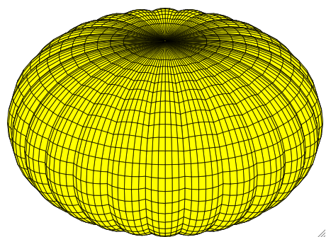
Figure 11: Complete pumpkin.

The EVA vehicle will be a super-pressure pumpkin balloon now in development by NASA’s Balloon Program Office. See Fig. 11 for an illustration of a pumpkin balloon consisting of 24 gores. The actual EVA pumpkin will likely be made of 230 or more gores. The lobes will be shallower, but still noticeable. In order to fully understand the geometry of such a structure it will be beneficial to calculate curvatures for such a shape.

The design program Planetary Ballon RF developed by R. Farley, NASA/GSFC will be used to determine the gore cutting pattern for the actual EVA balloon. In Planetary Balloon, mechanical properties of the balloon film and load tendons are used to estimate the strained shape of a pumpkin lobe under certain design conditions. The flat cutting pattern for the gore is then backed out from this strained shape. To analyze the strained EVA balloon, we will use the analytical balloon model developed by Baginski (see, e.g., BBC ). However, to simplify the exposition of the pumpkin geometry, we will assume the complete shape is cyclically symmetric and made of ${n_{g}}$ symmetric lobes and smooth within each lobe. Within a typical gore, ${\bf x}(u,v)$ is a parametrization of a tubular surface with generating curve $\Gamma$ defined by an Euler-Elastica curve (to be defined in the next section). Proceeding in this fashion, we obtain a fairly accurate representation of the equilibrium surface of a pressurized pumpkin balloon constrained by load tendons with a suspended payload BagSIAP05 . The tubular surface parametrization will facilitate the discussion of balloon surface properties that are relevant to antenna applications.

Euler-Elastica

The Euler-Elastica curve is the planar curve $(x,z)=(r(s),z(s))$ for $0<s<\ell$ satisfying BagSIAP05

$$\theta^{\prime\prime}+2\tau\sin\theta=0,$$ (1.1)

where $\theta$ is the angle between the tangent of the generating curve ${\bf t}=(r^{\prime}(s),z^{\prime}(s))=(\sin\theta,\cos\theta)$ and ${\bf k}=(0,0,1)$. In this model, we set the film weight density and tendon weight densities to zero (but include their total weight into the suspended payload) and set $\tau=\pi p_{0}/T_{0}$ where $T_{0}$ is the total tension (due to payload plus system weight) and $p_{0}$ is the constant differential pressure. Typical boundary conditions set the curvature equal to zero at the endpoints, $\theta^{\prime}(0)=\theta^{\prime}(\ell)=0$. The modulus of the elliptic functions associated with a solution of Eq. (1.1) is normally taken to be $1/\sqrt{2}$. In Fig. 12, we compare a natural shape profile (used in the design of zero-pressure balloons) with an Euler-elastica profile.

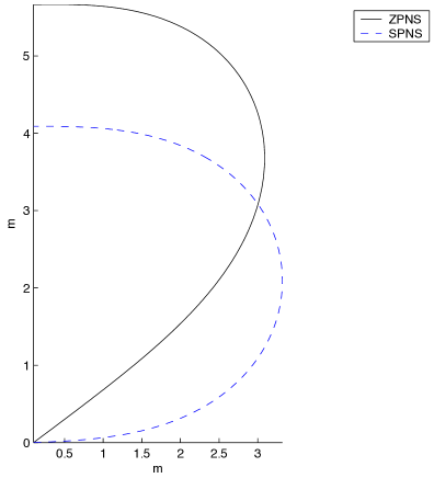
Figure 12: Comparison of a natural shape profile and the Euler-Elastica profile.

The radial component of the generating curve for the elastica is

$$r^{2}(\theta)=\tau^{-1}\sin({\textstyle{\frac{1}{2}}}\pi-\theta)$$ (1.2)

(see, Smc ) and the curvature of the elastica curve is $\kappa(s)=\theta^{\prime}(s)=-2\tau r(s)$ (see (BagSIAP05, , Sec. 2.3.2)). An expression for $z$ can be found by integrating $z^{\prime}(s)=\cos\theta$ or by using elliptic functions MladenovOprea .

Tubular Surface

We present the equations for a pumpkin shape balloon as a tubular surface. We assume that the pumpkin shape is made up of $n_{g}$ symmetric pumpkin gores. Let ${\bf i}=(1,0,0)$. We begin with a curve,

$$\mbox{\boldmath$\Upsilon$}(s)=r(s){\bf i}+z(s){\bf k}\in\mbox{I$\!$R}^{3},$$

that we call the generator of the pumpkin gore. We assume that $(r(s),z(s))$ is known from the solution of Eq. (1.1). $\Upsilon$ is parametrized by arc length $s$, i.e., $r^{\prime}(s)^{2}+z^{\prime}(s)^{2}=1$. Let ${\bf t}$ denote the unit tangent of $\Upsilon$, ${\bf b}$ its inward unit normal (${\bf j}={\bf t}\times{\bf b}$); as defined in Eq. (1.1), $\theta=\theta(s)$ is the angle between ${\bf t}$ and ${\bf k}$, and

$${\bf t}(s) = \sin\theta{\bf i}+\cos\theta{\bf j},$$

$${\bf b}(s) = -\cos\theta{\bf i}+\sin\theta{\bf j}.$$

The set $\{{\bf b},{\bf t},{\bf j}\}$ gives a right hand curvilinear basis for $\mbox{I$\!$R}^{3}$. Since $\Upsilon$ is a plane curve, its torsion is zero, and the Frenet equations reduce to

$${\bf t}^{\prime}(s) = \kappa(s){\bf b}(s),$$

$${\bf b}^{\prime}(s) = -\kappa(s){\bf t}(s)$$

where $\kappa$ is the curvature of $\Upsilon$ (see (doCarmo, , Sec. 1.5)). We define a tubular surface in the following manner. For $-\pi<v<\pi,\ \ 0<s<\ell$, let

$${\bf x}(s,v)=\mbox{\boldmath$\Upsilon$}(s)+{r_{b}}\left(-{\bf b}(s)\cos v+{\bf j}\sin v\right),\ \$$ (1.3)

and $x(s,v)={\bf x}(s,v)\cdot{\bf i},y(s,v)={\bf x}(s,v)\cdot{\bf j}$, and $z(s,v)={\bf x}(x,v)\cdot{\bf k}$.

By direct calculation, we have

$${\bf x}_{s}(s,v) = (1+{r_{b}}\kappa(s)\cos v){\bf t}(s),$$

$${\bf x}_{v}(s,v) = {r_{b}}\left({\bf b}(s)\sin v+{\bf j}\cos v\right),$$

$${\bf x}_{s}\times{\bf x}_{v} = {r_{b}}(1+{r_{b}}\kappa(s)\cos v)$$

$$\ \ \ \cdot\left({\bf b}(s)\cos v-{\bf j}\sin v\right),$$

and area measure is $dS={r_{b}}(1+{r_{b}}\kappa(s)\cos v)dsdv$. A unit vector normal to the tubular surface is

$${\bf N}(s,v)={\bf x}_{s}\times{\bf x}_{v}/|{\bf x}_{s}\times{\bf x}_{v}|={\bf b}(s)\cos v-{\bf j}\sin v.$$

The triple $\{{\bf x}_{s},{\bf x}_{v},{\bf N}\}$ gives a right hand basis for $\mbox{I$\!$R}^{3}$. Further calculation yields,

$${\bf N}_{s}(s,v) = -\kappa(s){\bf t}(s)\cos v$$

$${\bf N}_{v}(s,v) = -{\bf b}(s)\sin v+{\bf j}\cos v.$$

The principal curvatures are

$$\kappa_{1}(s,v) = -\frac{{\bf N}_{s}\cdot{\bf x}_{s}}{{\bf x}_{s}\cdot{\bf x}_{s}}=\frac{\kappa\cos v}{1+{r_{b}}\kappa\cos v},$$ (1.4)

$$\kappa_{2}(s,v) = -\frac{{\bf N}_{v}\cdot{\bf x}_{v}}{{\bf x}_{v}\cdot{\bf x}_{v}}=\frac{1}{{r_{b}}}.$$ (1.5)

The tubular surface is sufficiently smooth whenever (see (doCarmo, , p. 399))

$${r_{b}}\kappa_{0}<1,\mbox{ \ where \ }\kappa_{0}<\max_{0\leq s\leq\ell}|\kappa(s)|.$$ (1.6)

Condition Eq. (1.6) is met in our applications.

A unit tangent to the curve $s\rightarrow{\bf x}(s,v)$ is

$${\bf a}_{1}(s,v)={\bf x}_{s}(s,v)/|{\bf x}_{s}(x,v)|={\bf t}(s),$$

and a unit tangent to the curve $v\rightarrow{\bf x}(s,v)$ is

$${\bf a}_{2}(s,v)={\bf x}_{v}(s,v)/|{\bf x}_{v}(s,v)|={\bf b}(s)\sin v+{\bf j}\cos v.$$

Note, ${\displaystyle\frac{\partial{\bf a}_{2}}{\partial v}={\bf b}(s)\cos v-{\bf j}\sin v={\bf N}.}$ In Figure 13, the geometry of a pumpkin gore patch is illustrated with the vectors $\{{\bf a}_{1},{\bf a}_{2},{\bf N}\}$ when $v=0$.

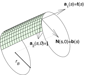
Figure 13: A pumpkin gore with $\{{\bf a}_{1},{\bf a}_{2},{\bf N}\}.$

Arc length in the tubular surface along a curve parallel to the generator $s\rightarrow{\bf x}(s,v)$ is $\bar{s}$, where $d\bar{s}=(1+{r_{b}}\kappa(s)\cos v)ds.$

A pumpkin gore will be a subset of a tubular surface. We assume that the pumpkin gore is situated symmetrically with respect to the $xz$ plane and interior to the wedge defined by the half-planes $y=\pm\tan(\pi/{n_{g}})x$ with $x\geq 0$. See Fig. 14. We will refer to ${r_{b}}$ as the bulge radius of the pumpkin gore. The curve traced by $v\rightarrow\mbox{\boldmath$\Upsilon$}(s)+{r_{b}}(-{\bf b}(s)\cos v+{\bf j}\sin v)$ is a circle lying in the plane with normal ${\bf t}(s)$. To find the length of the segment of the circle that forms a circumferential arc of the pumpkin gore, we need to find the values of $v$ where this arc intersects the planes $y=\pm\tan(\pi/{n_{g}})x$. For fixed $s$, we find that $v$ must satisfy the condition

$$y(s,v)=\tan(\pi/n_{g})~{}x(s,v).$$

This leads us to the equation

$$A(s)+B(s)\cos v+C\sin v=0,$$ (1.7)

where $C={r_{b}}$, $B(s)=-{r_{b}}\cos\theta(s)\tan(\pi/{n_{g}})$, and $A(s)=-R(s)\tan(\pi/{n_{g}})$. Eq. (1.7) can be solved for $v$, yielding

$$v=v_{g}=\arccos\left(\frac{-AB+C{\sqrt{C^{2}+B^{2}-A^{2}}}}{B^{2}+C^{2}}\right).$$

Since $A$ and $B$ are functions of $s$ and other parameters, so is $v_{g}=v_{g}(s,n_{g},R(s),\theta(s))$. By symmetry, the solution corresponding to the plane $y=-\tan(\pi/{n_{g}})x$ is $v=-v_{g}$. We define the three dimensional pumpkin gore ${\sl G}$ to be the set,

$${\sl G}=\left\{{\bf x}(s,v),\ \ -v_{g}(s)<v<v_{g}(s),\ \ 0<s<\ell\right\}.$$

A complete shape ${\cal S}$ has cyclic symmetry and is made up of ${n_{g}}$ copies of ${\sl G}$. In Fig. 11, we present a pumpkin balloon with ${n_{g}}=24$, ${r_{b}}=10.9$ m, and $\max r=55.77$ m. Fig. 11 was for demonstration purposes only.

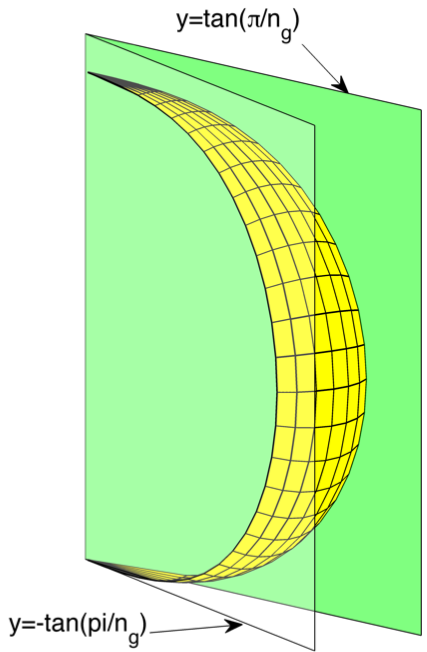
Figure 14: Pumpkin lobe.

Case Study

It will be beneficial to consider a pumpkin balloon of sufficient size for an EVA-type payload. This leads to a balloon design that we can approximate as a tubular surface as given by Eq. (1.3) with ${n_{g}}=230$ and ${r_{b}}=2.7$ meters. In this case we find the maximum radius of the generating curve is $\max r=58$ meters and $H=\max z=69.49$ m. In Figure 15, we present the generating curve $(r(s),z(s))$ where $0<s<\ell=302.6$ m for the Euler-elastica $\Upsilon$ as described. In Figure 16, we present $(z(s),\kappa(s))$. In Table 3, we present a few data points located with $\pm 3.88$ meters of the equatorial plane. $d(z,z_{0})$ measures the distance from the point $(r(z),z)$ to the equatorial plane $z=z_{0}=34.74$ m. $\kappa(z)$ is the principle curvature at $z$.

If we rotate the generating curve $\Upsilon$ about the $z$ axis, the resulting surface will have principle curvatures $\kappa$ and $\tilde{\kappa}$. The equatorial bulge angle is $2v_{b}(z_{eq})=27.2$ deg. This corresponds to an arc of $\Upsilon$ of approximately 11 meters in length.

A peculiarity of the surface of revolution generated by an Euler-Elastica is that its principal curvatures $\kappa_{m},\kappa_{h}$ satisfy $\kappa_{m}(s,v)=\frac{1}{2}\kappa_{h}(s,v)$. This is equivalent to the relation $R_{h}=2R_{m}$ where $\kappa_{m}=1/R_{m}$ and $\kappa_{h}=1/R_{h}$. Such a shape is the basis for the popular mylar balloons and is discussed in great detail in MladenovOprea . See Table 3. These observations will be of importance for the design of the focusing reflector.

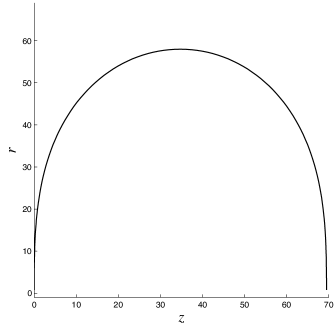
Figure 15: Euler-Elastica generator: $(z(s),r(s))$.

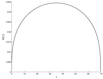
Figure 16: $(z(s),\kappa(s))$ for $0<s<\ell$.

Table 3: Surface data in an equatorial band.

(m)	(m)	(m)	(m)	(deg)
$d(z,z_{eq})$	$r(z)$	$R_{m}$	$R_{h}$	$v_{b}(z)$
-3.8821	57.7392	29.1310	58.2620	13.541
-2.5924	57.8839	29.0581	58.1163	13.575
-1.2975	57.9710	29.0145	58.0291	13.596
0	58.0000	29.0000	58.0000	13.603
1.2975	57.9710	29.0145	58.0291	13.596
2.5924	57.8839	29.0581	58.1163	13.575
3.8821	57.7392	29.1310	58.2620	13.541

References

- (1) V. S. Beresinsky and G. T. Zatsepin, Phys. Lett. B 28, 423 (1969).
- (2) D. Seckel and T. Stanev, Phys. Rev. Lett. 95 (2005) 141101.
- (3) R. Engel, D. Seckel, & T. Stanev, ”Neutrinos from propagation of ultra-high energy protons,” 2001, Bartol Research Institute Report Number BA-01-01 (astro-ph/0101216) and references therein provides a recent comprehensive summary of the GZK neutrino connection.
- (4) “Observation of the GZK Cutoff Using the HiRes Detector,” D.R. Bergman (presented on behalf of the High Resolution Fly’s Eye Collaboration) Comments: 8 pages, 12 figures. Proceedings submission for CRIS 2006, Catania, May/June 2006 Journal-ref: Nucl.Phys.Proc.Suppl.165:19-26,2007
- (5) J. Abraham et al. [The Pierre Auger Collaboration], “Observation of the Suppression of the Flux of Cosmic Rays above eV” Phys. Rev. Lett. 101, 061101 (2008).
- (6) Schuessler, F. [Auger Collaboration], “Measurement of the cosmic ray energy spectrum above eV using the Pierre Auger Observatory,” Phys. Lett. B, 2009, in press. (arXiv:1002.1975).
- (7) K. Greisen, ”End to the Cosmic Ray Spectrum?,” Phys. Rev Lett. 16,748 (1966).
- (8) G.T. Zatsepin and V. A. Kuz’min, JETP Letters 4, 78 (1966).
- (9) V. S. Beresinsky and G. T. Zatsepin, Phys. Lett. B 28, 423.
-
(10)
C.T. Hill and D, N. Schramm, ”Ultrahigh-energy cosmic-ray
spectrum,” Phys. Rev. D 31,564 (1985); F.W. Stecker,
”Effect of Photomeson Production by the Universal Radiation Field on
High-Energy Cosmic Rays,” Phys. Rev. Lett. 21, 1016-1018 (1968).
- (11) J. Linsley, Phys. Rev. Lett. 10, 146 (1963); see also Proc. of the Int’l Cosmic Ray conference, Jaipur 1963, ed. R. Daniel et al., (Commercial Press, Bombay), vol. IV, 77.
- (12) D. J. Bird et al.,”Evidence for Correlated Changes in the Spectrum and Composition of Cosmic Rays at Extremely High Energies,” Phys. Rev. Lett. 71, 3401 (1993); H. Hayashida et al., Ap. J. 522, 225 (1999); C. C. H. Jui et al., 26th International Cosmic Ray Conference Invited, Rapporteur, and Highlight papers (AIP Conf. Proc 516), 370 (2000).
-
(13)
T.Abu-Zayyad, at. al., ”Measurement of the Cosmic
Ray Energy Spectrum and Composition from to eV Using a
Hybrid Fluorescence Technique”, Astrophys. J. 557, 686
(2001).
- (14) M. Takeda et al., Astroparticle Physics 19, 447-462 (2003).
- (15) P. L. Biermann and P. A. Strittmatter, Astrophys. J. 322, 643 (1987); J. P. Rachen and P. L. Biermann, Astron. Astrophys. 272, 161 (1993).
- (16) E. Waxman, Phys. Rev. Lett. 75, 386 (1995); E. Waxman, Astrophys. J. 606, 988 (2004); M. Vietri, Astrophys. J. 453, 883 (1995); M. Vietri, D. De Marco and D. Guetta, Astrophys. J. 592, 378 (2003); C. D. Dermer, Astrophys. J. 574, 65 (2002); C. D. Dermer and M. Humi, Astrophys. J. 556, 479 (2001).
- (17) J. P. U. Fynbo et al., Astron. Astrophys. 406, L63 (2003); J. X. Prochaska et al., Astrophys. J. 611, 200 (2004); J. Gorosabel et al., Astron. Astrophys. 444, 711 (2005); P. Jakobsson et al., Mon. Not. Roy. Astron. Soc. 362, 245 (2005); J. Sollerman, G. Ostlin, J. P. U. Fynbo, J. Hjorth, A. Fruchter and K. Pedersen, New Astron. 11, 103 (2005).
- (18) G. A. Askaryan, JETP 14, 441 (1962); also JETP 21, 658 (1965).
- (19) D. Saltzberg, P. Gorham, D. Walz, et al., “Observation of the Askaryan Effect: Coherent Microwave Cherenkov Emission from Charge Asymmetry in High Energy Particle Cascades,” Phys. Rev. Lett., 86, 2802 (2001).
- (20) P. W. Gorham, D. P. Saltzberg, P. Schoessow, et al., “Radio-Frequency Measurements of Coherent Transition and Cherenkov Radiation: Implications for High-Energy Neutrino Detection,” Phys. Rev. E. 62, 8590 (2000).
- (21) P. W. Gorham, D. Saltzberg, R. C. Field, E. Guillian, R. Milincic, D. Walz, D. Williams, “Accelerator Measurements of the Askaryan effect in Rock Salt: A Roadmap Toward Teraton Underground Neutrino Detectors,” Phys.Rev. D72 (2005) 023002; http://arxiv.org/abs/astro-ph/0412128v2
- (22) The ANITA Collaboration, P. W. Gorham, S. Barwick, J. Beatty, et al., “Observations of the Askaryan Effect in Ice,” Phys. Rev. Letters, (2007) in final revision; http://arxiv.org/abs/hep-ex/0611008 .
- (23) P. Miočinović, R. C. Field, P. W. Gorham, et al., “Time-Domain Measurement of Broadband Coherent Cherenkov Radiation,” Phys. Rev. D 74, 043002 (2006).
- (24) K. S. Kelleher, and H. H. Hibbs, “A new Microwvae Reflector,” Naval Research Laboratory Report No. 4141, May 1953.
- (25) G. D. M. Peeler, and D. H. Archer, ”A Toroidal Wave Reflector,” IRE Convention Record, 1954, 242-247.
- (26) R. C. Johnson and H. Jasik, Antenna Egineering Handbook, (McGraw-Hill: New York), 2nd edition, 1984.
- (27) E. A. Wolff, Antenna Analyis, (Wiley and Sons: New York), first edition, 1966.
- (28) Gorham, P. W. et al., “The Antarctic Impulsive Transient Antenna ultra-high energy neutrino detector: Design, performance, and sensitivity for the 2006-2007 balloon flight,” Astropart. Phys. 32, 10-41 (2009).
- (29) G. A. Gusev, I. M. Zheleznykh, “On the possibility of detection of neutrinos and muons on the basis of radio radiation of cascades in natural dielectric media (antarctic ice sheet and so forth),” SOV PHYS USPEKHI, 1984, 27 (7), 550-552.
- (30) ”Predictions for the Cosmogenic Neutrino Flux in Light of New Data from the Pierre Auger Observatory,” Luis A. Anchordoqui, Haim Goldberg, Dan Hooper, Subir Sarkar, Andrew M. Taylor Phys. Rev. D76: 123008, 2007.
- (31) O. E. Kalashev, et al.,Phys. Rev. D66, 063004 (2002).
- (32) R. J. Protheroe & P. A. Johnson, Astropart. Phys. 4 (1996) 253.
- (33) C. Aramo et al., Astropart. Phys. 23 (2005) 65.
- (34) E. Waxman and J. N. Bahcall, Phys. Rev. D 59, 023002 (1999); J. N. Bahcall and E.Waxman, Phys. Rev. D 64, 023002 (2001).
- (35) F. Baginski, W. Collier, and T. Williams, ”A PARALLEL SHOOTING METHOD FOR DETERMINING THE NATURAL SHAPE OF A LARGE SCIENTIFIC BALLOON,” SIAM J. APPL. MATH (1998), Vol. 58, No. 3, pp. 961.
- (36) F. Baginski, ”ON THE DESIGN AND ANALYSIS OF INFLATED MEMBRANES: NATURAL AND PUMPKIN SHAPED BALLOONS” SIAM J.PL. MATH. (2005) Vol. 65, No. 3, pp. 838.
- (37) Baginski, F. & Brakke K., “Estimating the deployment pressure in pumpkin balloons,” AIAA Journal of Aircraft, Vol. 48 (1), 2011, 235-247.
- (38) H. M. Cathey, “The NASA Super Pressure Balloon. A Path to Flight,” Advances in Space Research Vol. 44, Issue 1, 1 July 2009, Pages 23-38.
- (39) Chu, T. S. and Iannone, P.P. , “Radiation properties of parabolic torus reflector,” IEEE Transactions on Antennas and Propagation, 1989, Volume: 37 Issue: 7, 865 - 874
- (40) G.S. Varner, L.L. Ruckman and A. Wong, “The First version Buffered Large Analog Bandwidth (BLAB1) ASIC for high luminosity collider and extensive radio neutrino detectors,” Nucl. Instr. Meth. A591 (2008) 534-545.
- (41) G.S. Varner, L.L. Ruckman, R.J. Nichol, J. Nam, J. Cao, M. Wilcox and P. Gorham, “Large Analog Bandwidth Recorder and Digitizer with Ordered Readout (LABRADOR) ASIC,” Nucl. Instr. Meth. A483 (2007) 447-460.
- (42) D. Ball, D. Pierce, and D. Gregory, personal communication 2010.
- (43) P. Gorham et al. [the ANITA collaboration] “Observational Constraints on the Ultra-high Energy Cosmic Neutrino Flux from the Second Flight of the ANITA Experiment,” Phys. Rev. D82, 022004 (2010).
- (44) G. Burke, A. Poggio, J. Logan, J. Rockway, “NEC - Numerical Electromagnetics code for Antennas and Scattering,” Antennas and Propagation Society International Symposium, 1979, 17:147-150.
- (45) H. M. Cathey, 2011, personal communication.
- (46) H. Yuksel, M. D. Kistler “Implications of a GRB-Metallicity Anti-Correlation for Cosmogenic Neutrinos”, PRD, 2007 in press; astro-ph/0610481.
- (47) S. Yakoob et al., ”Transmission performance assessment for WLAN Direct Modulation Radio over Fiber System,” Proceedings of the International Conference on Electrical Engineering and Informatics, Institut Teknologi Bandung, Indonesia June 17-19, 2007.
- (48) E.I. Ackerman, C.H. Cox, ”RF fiber-optic link performance,” Microwave Magazine, Vol. 2 Issue 4, Dec. 2001, 50-58.
- (49) R. Beresford, ”ASKAP photonic requirements,” Microwave Photonics, Sept. 9 2008, 62-65.
- (50) ”The World’s Highest Electro-Optical Conversion Efficiency of 62in Vertical Cavity Surface Emitting Lasers (VCSELs) Has Been Achieved,” retrieved March 23, 2009. http://www.furukawa.co.jp/english/what/2008/kenkai_081219.htm
- (51) S. Hoover et al. [ANITA Collaboration] “Observation of Ultra-high-energy Cosmic Rays with the ANITA Balloon-borne Radio Interferometer ,” Phys. Rev. Lett. 105, 151101, (2010).
- (52) Baginski, F., Barg, M, Collier, W., Existence Theorems for Tendon Reinforced Thin Wrinkled Membranes Subjected to a Hydrostatic Pressure, Mathematics and Mechanics of Solids, 13(6), 532-570, 2008.
- (53) F. Baginski, On the design and analysis of inflated membranes: natural and pumpkin shaped balloons, SIAM Journal on Applied Mathematics, 65 (3) 838-857, 2005.
- (54) Manfredo P. do Carmo, Differential Geometry of Curves and Surfaces, Prentice-Hall, Englewood Cliffs, New Jersey, 1976.
- (55) R. Farley, Planetary Balloon: Balloon Design Software Manual, NASA Goddard Space Flight Center, Greenbelt, MD, 2007.
- (56) I. Mladenov and J. Oprea, The mylar balloon revisited, MAA Monthly, 110 Nov 2003, p. 761-784
- (57) J. H. Smalley, Development of the e-balloon, AFCRL-70-0543, National Center for Atmospheric Research, Boulder, Colorado, June 1970
- (58) H. Cathey, Adv. in Space Res. 44 (2009) 23–38.