Gamma-ray emission of accelerated particles escaping a supernova remnant in a molecular cloud

Abstract

We present a model of gamma-ray emission from core-collapse supernovae originating from the explosions of massive young stars. The fast forward shock of the supernova remnant (SNR) can accelerate particles by diffusive shock acceleration (DSA) in a cavern blown by a strong, pre-supernova stellar wind. As a fundamental part of nonlinear DSA, some fraction of the accelerated particles escape the shock and interact with a surrounding massive dense shell producing hard photon emission. To calculate this emission, we have developed a new Monte Carlo technique for propagating the cosmic rays (CRs) produced by the forward shock of the SNR, into the dense, external material. This technique is incorporated in a hydrodynamic model of an evolving SNR which includes the nonlinear feedback of CRs on the SNR evolution, the production of escaping CRs along with those that remain trapped within the remnant, and the broad-band emission of radiation from trapped and escaping CRs. While our combined CR-hydro-escape model is quite general and applies to both core collapse and thermonuclear supernovae, the parameters we choose for our discussion here are more typical of SNRs from very massive stars whose emission spectra differ somewhat from those produced by lower mass progenitors directly interacting with a molecular cloud.

I. Introduction

Many core-collapse supernovae are expected to explode within their parent molecular clouds. Because of the influence of the surrounding material, the manifestation of the supernova remnant (SNR) can differ substantially depending on the progenitor star type. For a relatively low progenitor mass below $\sim 12$-14 $\mathrm{M}_{\odot}$, the stellar wind and photoionizing radiation are not sufficient to substantially clear out the surrounding cloud and already at a radius of about 6 pc the remnant can enter a radiative phase with a shock directly interacting with the molecular cloud (e.g., Chevalier, 1999). The radiative shock with a typical velocity below $\sim 150$ km s^-1 can accelerate and compress CRs and produce non-thermal radiation (Bykov et al., 2000; Uchiyama et al., 2010). Recently, the Large Area Telescope on board the Fermi Gamma-Ray Space Telescope detected GeV emission from SNRs IC 443, W44, and 3C 391 known to be directly interacting with molecular clouds (see, e.g., Abdo et al., 2010b, a; Castro & Slane, 2010).

Higher mass young stars with masses above $\sim 16\,\mathrm{M}_{\odot}$ (of B0 V type and earlier) are likely to create low-density bubbles and HII regions with radii $\sim 10$ pc surrounded by a massive shell of matter swept up from the molecular cloud by the wind and the ionizing radiation of the star over its lifetime. In this case, a strong supernova shock propagates for a few thousand years in tenuous circumstellar matter with a velocity well above $10^{3}$ km s^-1 before reaching the dense massive shell where it decelerates rapidly.

Regardless of the SN type, the blast wave of the SNR is expected to accelerate ambient material and generate relativistic electrons and ions, i.e., cosmic rays (CRs), which produce strong non-thermal radiation. A preponderance of evidence suggests that the particle acceleration mechanism most likely responsible is diffusive shock acceleration (DSA) (e.g., Blandford & Eichler, 1987; Jones & Ellison, 1991; Malkov & Drury, 2001).

We note that despite the common acceleration mechanism, the appearance of the two classes of SNRs we mention can differ very substantially. For early progenitor stars, one can expect that a sizeable fraction of the $\gamma$-ray emission is produced by the CR ions that escape the forward shock and interact with the dense surrounding shell, while for lower mass progenitors, the bulk of the non-thermal radiation is likely to come from trapped CRs.

While the CRs produced by the SNR generate non-thermal emission across the spectrum from radio to TeV $\gamma$-rays, the $\gamma$-rays are of particular interest because they may be produced in proton-proton (or heavier ion) collisions of ultra-relativistic particles. In fact, there are three populations of shock accelerated CRs that are important for producing $\gamma$-rays: relativistic electrons producing $\gamma$-rays through inverse-Compton and non-thermal bremsstrahlung; CR ions that remain trapped within the forward shock precursor; and CR ions that are accelerated by the forward shock but escape upstream. These three populations are produced simultaneously by DSA but they have very different properties and will have very different $\gamma$-ray signatures.

As has been known for some time (e.g., Ellison, Jones & Eichler, 1981; Eichler, 1984; Ellison & Eichler, 1984; Berezhko & Krymskii, 1988), a large fraction of the energy in particles accelerated at strong shocks can escape at an upstream boundary. In fact, the fraction of all galactic CRs that originate as escaping particles is likely to be significant and escaping CRs may even provide the bulk of CRs at the “knee” and above. The importance of modeling escaping CRs was discussed before the advent of DSA (e.g., Schwartz & Skilling, 1978) and is attracting considerable attention currently within the DSA paradigm (see, e.g., Ptuskin & Zirakashvili, 2005; Caprioli, Amato & Blasi, 2010; Drury, 2010). Recently, Reville, Kirk & Duffy (2009) used a simple iterative scheme to construct stationary numerical solutions to the coupled kinetic and hydrodynamic DSA equations. The stationary solutions with efficient acceleration were found when the escape boundary was placed at the point where the growth and advection of strongly driven, non-resonant waves where in balance. For that particular case, they derived the energy dependence of the distribution function close to the energy break. As we shall argue below, some additional factors, e.g., stochastic Fermi acceleration on long-wavelength fluctuations, can affect the spectral shape of the escaping particles.

A number of stationary, nonlinear (NL) models of DSA can provide the integrated escaping CR energy flux as a fraction of the parameterized overall acceleration efficiency, but no model is yet able to determine the spectral shape of escaping CRs taking into account the self-consistent production of magnetic instabilities produced by both the trapped CRs in the shock precursor and the escaping CRs. Such a treatment is not yet feasible, creating an important problem since the interpretation of the $\gamma$-ray emission from young SNRs depends critically on the uncertain spectral shape of both the trapped and escaping CRs. Therefore, a suitable parameterization of the shape of the escaping CR flux is needed to allow comparisons with $\gamma$-ray observations of young SNRs in the hope of constraining NL DSA models.

It is important to note, of course, that SNRs are not stationary and the dynamics of an expanding remnant, even in the simplest spherical case, adds an additional factor to the issue of CR escape. As the remnant expands, the precursor region beyond the forward shock that is filled with CRs expands producing a “dilution” of CR energy density. This effect has been studied in detail by Berezhko and co-workers (e.g., Berezhko, Elshin, & Ksenofontov, 1996a, b) (see also Drury, 2010). In a real shock, the dilution effect is coupled to escape since the lowering of the CR energy density results in less efficient generation of magnetic turbulence and this will change the escape of CRs. Both the flow of energy out of the shock by escape and the dilution of the CR energy density influence the Rankine-Hugoniot conservation relations in similar ways. Both act as energy sinks and both result in an increase in the shock compression and other nonlinear effects. In the stationary, plane-shock approximation for DSA used here, we ignore dilution and only include the escape of CRs at an upstream free escape boundary. It has been shown, however, that this plane-shock approximation gives essentially the same results for the shock structure as in a spherical, expanding shock if the specific mode of escape is unimportant (see Berezhko & Ellison, 1999). The mode of escape becomes important, however, if the escaping CR flux is used to calculate $\gamma$-ray emission in material external to the shock. Since we neglect dilution, our escaping CR fluxes, and the $\gamma$-ray emission we calculate from them, are over estimated.

In this paper, we present a new Monte Carlo technique for propagating escaping CRs and calculating their $\gamma$-ray production via pion-decay, in the circumstellar medium (CSM) surrounding the outer SNR blast wave. This treatment of escaping CRs is added to our CR-hydro simulation (e.g., Ellison, Decourchelle & Ballet, 2005; Ellison et al., 2010, and references therein) producing a coherent model where a number of related elements of the SNR are treated more or less self-consistently. The hydrodynamic simulation couples the efficient production of CRs to the SNR evolution, including the production of escaping CRs as an intrinsic part of the DSA process. The escaping CRs are emitted from the forward shock as the SNR evolves, their propagation is followed as they diffuse in the CSM, and the $\gamma$-ray emission of these CRs is calculated consistently with that from the CRs (protons and electrons) that remain trapped within the remnant. While a number of important approximations are required, including the neglect of precursor CR dilution, this model represents a fairly complete and internally self-consistent description of a SNR interacting with a non-homogeneous CSM.

The importance of freshly made CRs interacting with their local environment to produce $\gamma$-rays has been recognized for some time and an extensive literature exists in this field. In a generalization of the model of Gabici & Aharonian (2007) (and previous work, e.g., Aharonian & Atoyan, 1996), Gabici, Aharonian & Casanova (2009) calculate the broad-band emission, from radio to TeV $\gamma$-rays, from CRs produced by a SNR interacting with a nearby molecular cloud. They emphasize that, depending on the parameters, the $\gamma$-ray emission can exceed other bands by a large factor, suggesting that some unidentified TeV sources might be associated with clouds illuminated by nearby SNRs. Gabici, Aharonian & Casanova (2009) also note the importance of the shape of the $\gamma$-ray spectrum for identifying GeV-TeV sources.

The model used by Gabici, Aharonian & Casanova (2009) is based on that of Ptuskin & Zirakashvili (2005) and includes a description of the evolution of the SNR and the spectrum of escaping CRs. In Gabici, Aharonian & Casanova (2009), the important parameter $p_{\mathrm{max}}$, the maximum cutoff momentum for the CR spectrum, is parameterized as $p_{\mathrm{max}}(t)\propto t^{-\delta}$, where $t$ is the age of the SNR and $\delta$ is taken to be $\sim 2.48$ to match the CR data below the knee, as measured at Earth. Our parameterization of $p_{\mathrm{max}}$ differs considerably from this as we discuss below. An important result of Ptuskin & Zirakashvili (2005) (see Berezhko & Krymskii, 1988, for an earlier derivation) that is incorporated in the Gabici, Aharonian & Casanova (2009) model and is not modeled here is that, when integrated over the whole Sedov phase, the total CR spectrum is a power law of the form $F_{\mathrm{esc}}\propto p^{-4}$. Recently, Casanova et al. (2010) have applied the Gabici, Aharonian & Casanova (2009) model to SNR RX J1713.7-3946 taking into account the details of the ambient gas distribution.

The model presented here is similar to that of Lee, Kamae & Ellison (2008). In both cases, the evolving SNR is modeled with a spherically symmetric hydrodynamic simulation where the efficient production of CRs via DSA is coupled to the remnant dynamics. The main difference is in the treatment of the diffusion of escaping CRs in the region beyond the SNR forward shock. The work of Lee, Kamae & Ellison (2008) uses a “boxel” technique whereby, at each time step and each spatial grid in the 3D simulation box, particles are exchanged between the adjacent boxels according to the particle momentum, location, and density gradient. In the model presented here, we use a Monte Carlo technique to propagate escaping CRs in the region beyond the forward shock. These two methods of propagation have distinct advantages and disadvantages, and both differ importantly from more analytic models based on a direct solution of a diffusion equation. In any case, we feel the problem of CRs produced by relatively young SNRs interacting with dense, local material is important enough to be considered with a variety of complementary techniques.

Other differences between the boxel model of Lee, Kamae & Ellison (2008) and our new Monte Carlo model are all based on recent refinements of the CR-hydro model (see Ellison et al., 2010, and references therein) and on how we parameterize the escaping CR distribution, described below. While these refinements are important for modeling specific remnants, they do not substantially change the results given in Lee, Kamae & Ellison (2008).

II. Model

The model we present here consists of two main parts. The CR-hydro part is used to calculate the evolution of a SNR and is essentially the same as that described in Ellison et al. (2007), Patnaude, Ellison & Slane (2009), Ellison et al. (2010) and references therein. The evolution of the spherically symmetric remnant is coupled to the efficient production of CRs and the production of thermal and non-thermal emission is calculated (see Ellison et al., 2010, for recent work modeling the broad-band emission from SNR RX J1713.7-3946). The diffusive shock acceleration is determined in the CR-hydro model using the semi-analytic model of Blasi and co-workers (e.g., Blasi, 2002; Amato & Blasi, 2005; Blasi, Gabici & Vannoni, 2005). The injection scheme for this model has been discussed in detail in a number of previous papers (see Caprioli, Amato & Blasi, 2010, for recent extensions of the model) but we note that we use a slightly different injection method than typically used by Blasi and co-workers. Since the diffusion approximation upon which the semi-analytic model is based doesn’t apply to thermal particles, a parameter, $\eta_{\mathrm{inj}}$, must be defined that specifies what fraction of thermal particles obtain a superthermal energy and are injected into the DSA mechanism. Given this parameter, the nonlinear DSA mechanism determines the fraction of shock ram kinetic energy that goes into superthermal particles, i.e., the acceleration efficiency ${\cal E_{\mathrm{DSA}}}$. The only difference in our implementation of this injection model and that of Blasi and co-workers is that we specify ${\cal E_{\mathrm{DSA}}}$ and then set $\eta_{\mathrm{inj}}$ accordingly. Both schemes are approximations since, in an evolving SNR, both $\eta_{\mathrm{inj}}$ and ${\cal E_{\mathrm{DSA}}}$ are likely to be functions of age. For simplicity, we hold ${\cal E_{\mathrm{DSA}}}$ constant.

The Blasi et al. model that we use also implicitly assumes that the shock is planar and stationary. Apart from the neglect of CR dilution, this approximation will be reasonably accurate as long as the diffusion length of the highest energy CRs is a small fraction of the shock radius. The sharp X-ray synchrotron edges often seen in SNRs (e.g., Warren et al., 2005; Eriksen et al., 2011) implies the presence of amplified magnetic fields which will result in short diffusion lengths. In our models here we assume that the diffusion length of protons with maximum momentum $p_{\mathrm{max}}$ is 1/10 of the shock radius, a small enough value to validate the planar approximation yet allow $p_{\mathrm{max}}\sim 10^{4-5}\,m_{p}c$, consistent with most models of CR production in SNRs.

Accounting for escaping CRs is essential in efficient DSA and escaping CRs are implicitly included in Blasi’s semi-analytic description. However, until now we have not included them in the production of radiation in the remnant environment in our CR-hydro model. The neglect of radiation produced by escaping CRs is justified if the SNR is in a uniform CSM with no external density enhancements. In this case, the emission from trapped CRs interacting with the shocked material is always much greater than that produced by escaping CRs in the less dense, unshocked external medium (see Model B in Fig. 5).

The second and new part of our model is a calculation of the escaping CR distribution that emerges from the SNR forward shock and the propagation and interaction of these escaping CRs in a dense, spherically symmetric shell external to the SNR. Depending on the density of the external material, $\gamma$-rays produced by the escaping CRs can overwhelm those produced by trapped CRs, as emphasized by Gabici, Aharonian & Casanova (2009). We note that while here we restrict ourselves to spherical symmetry for the external mass distribution, it is straightforward to generalize the Monte Carlo technique to arbitrary mass distributions.

II.1. Escaping CR Distribution

As we make clear in describing our parameterized escaping CR model, both the fraction of energy in escaping CRs and their spectral shape are uncertain. However, while controversial for some years, the idea that some fraction of the most energetic particles in a shock undergoing DSA must escape, regardless of whether the shock is stationary or not, is now generally accepted although certain qualifications are still made (see Drury, 2010).

We believe that energetic particle escape is a fundamental and unavoidable part of DSA that must occur in all supercritical collisionless shocks regardless of $p_{\mathrm{max}}$ or time evolution because (1) observations and modeling of the Earth bow shock (e.g., Scholer el at., 1980; Mitchell et al., 1983; Ellison, Moebius & Paschmann, 1990) support escape, (2) particle escape is an intrinsic part of many particle-in-cell (PIC) simulations (e.g., Giacalone et al., 1997; Giacalone & Ellison, 2000), and (3) DSA requires self-generated turbulence to work over any reasonable dynamic range. Since CRs must interact with self-generated turbulence to be further accelerated, the highest energy CRs far upstream in the shock precursor will always lack sufficient turbulence to remain nearly isotropic and some fraction will escape. These escaping CRs will generate turbulence for the next generation of CRs, creating a bootstrap effect. As mentioned above, the dilution of CR energy density that occurs in spherical, expanding shocks will be coupled to CR escape through the magnetic turbulence generation.

Given the assumptions and approximations of the model, the semi-analytic description of Blasi, Gabici & Vannoni (2005) determines the energy in escaping CRs, $Q_{\mathrm{esc}}$, but does not determine the shape of the distribution. While other work does determine the shape (e.g., Vladimirov, Ellison & Bykov, 2006; Zirakashvili & Ptuskin, 2008; Caprioli, Amato & Blasi, 2010), the shape that results in these models depends importantly on arbitrary parameters and the assumptions made for the diffusion of the highest energy escaping CRs.

Since the shapes of the trapped and escaping CR distributions, at the highest accelerated energies, are critical for modeling both X-ray synchrotron emission and GeV-TeV $\gamma$-ray emission, we feel it is important to have a flexible, i.e., parameterized, model that can be compared to observations to provide information on the uncertain plasma processes until an adequate theory of self-generated turbulence in the presence of escaping particles is developed (see Bykov, Osipov & Ellison, 2011, for recent work on long-wavelength instabilities that may influence the maximum momentum CRs can obtain in a given shock).

As an example of the complexities that may exist, the amplified long-wavelength fluctuations discussed in Bykov, Osipov & Ellison (2011) may result in particle acceleration by the resonant second-order Fermi mechanism. The stochastic acceleration rate, $\tau_{\rm ac}^{-1}$, for particles with spatial diffusion coefficient $\kappa(p)$ in the shock precursor is $\tau_{\rm ac}^{-1}\propto v^{2}_{\rm ph}/\kappa(p)$, where $v_{\rm ph}$ is the phase velocity. While this rate may be below the first-order acceleration rate, it may still be high enough to influence the spectra shape at the highest particle energies achieved by first-order DSA. The spectral index of particles accelerated by the second-order Fermi mechanism depends on the parameter $\tau_{\rm ac}/T_{\rm esc}$, where $T_{\rm esc}$ is the escape time (e.g., Petrosian & Bykov, 2008). In the case of resonant stochastic particle acceleration by long-wavelength fluctuations, $\tau_{\rm ac}/T_{\rm esc}\propto M_{\rm a}^{2}/[k_{1}\,r_{g}(p_{\rm max})]$, where the characteristic wave number of the CR instability (c.f., Bell, 2004; Bykov, Osipov & Ellison, 2011) is

$$k_{1}=\frac{4\pi}{c}\frac{\overline{j^{\mathrm{cr}}}}{B}\ .$$ (1)

Here, $\overline{j^{\mathrm{cr}}}$ is the mean CR current, $r_{g}(p_{\rm max})$ is the CR gyroradius at $p_{\mathrm{max}}$ in the magnetic field $B$, and $M_{\rm a}$ is the forward shock Alfvénic Mach number.

Therefore, for a large enough precursor CR current, $\overline{j^{\mathrm{cr}}}$, as expected for efficient DSA, the parameter $\tau_{\rm ac}/T_{\rm esc}$ may influence the shape of the CR distribution in the spectral break region. For instance, if a shock of velocity $V_{\mathrm{sk}}$ produces a power-law spectrum of accelerated particles up to some maximum momentum and transfers a fraction $\eta$ of the shock ram pressure to CRs, then $\tau_{\rm ac}/T_{\rm esc}\propto\eta^{-1}\,(c/V_{\mathrm{sk}})\,$ with a weak dependence on the particle momentum. The smaller $\tau_{\rm ac}/T_{\rm esc}$, the larger is the second-order Fermi effect and preliminary work (A. Bykov, in preparation) suggests that $\tau_{\rm ac}/T_{\rm esc}\lesssim 100$ is needed to see a significant modification of the spectral shape. While more exact estimates are difficult, we might expect $\eta\gtrsim 0.5$ and $V_{\mathrm{sk}}\gtrsim 5000$ km s^-1 to produce a noticeable effect.

When the shock accelerated particles approach $p_{\mathrm{max}}$, they begin leaving the upstream region of the shock and the approximate power-law distribution of particles that remain in the shock turns over in a fashion that will depend on the diffusion coefficient of the highest energy particles. Whatever the plasma processes are for escaping particles, the shape of the escaping distribution, $F_{\mathrm{esc}}(p)$, is determined by how CRs leave the shock and is, therefore, coupled to the trapped distribution. Since no current model of self-generated turbulence adequately describes the diffusion of escaping CRs, the diffusion coefficient is generally assumed to be Bohm-like right up to $p_{\mathrm{max}}$ and independent of position relative to the shock.

Figure 1.— The curves in the top two panels show the forward shock radius, $R_{\mathrm{FS}}$, and speed, $V_{\mathrm{sk}}$, as a function of remnant age. Both $R_{\mathrm{FS}}$ and $V_{\mathrm{sk}}$ are determined directly from the hydro code and include the energy loss from escaping CRs and all adiabatic effects. The gradual change in slope indicates a broad transition between an ejecta-dominated early phase and the Sedov phase at later times. The third panel shows the fraction of SN explosion energy in all CRs along with the fraction going into escaping CRs. In the bottom panel, $p_{\mathrm{max}}$ from the CR-hydro simulation (solid curve) is compared to that used in Gabici, Aharonian & Casanova (2009) (dashed curve). While the curves in this figure extend to $10^{4}$ yr, the simulations discussed in the remainder of this paper stop at $t_{\mathrm{SNR}}=1000$ yr, well before the SNR is fully in the Sedov phase. We note that the near identity of the CR-hydro and Gabici, Aharonian & Casanova (2009) value of $p_{\mathrm{max}}$ at $1000$ yr is essentially a coincidence. The parameters used for these results are listed as Model B in Table 1 but the quantities displayed here apply to all of our examples.

Here, we parameterize the escaping CR phase-space distribution, $F_{\mathrm{esc}}(p)$, as a modified parabola centered at $p_{\mathrm{max}}$, where $p_{\mathrm{max}}$ is the maximum momentum CRs would obtain if the acceleration cut off sharply when the upstream diffusion length, $\kappa(p_{\mathrm{max}})/V_{\mathrm{sk}}=L_{\mathrm{FEB}}$, where $V_{\mathrm{sk}}$ is the speed of the FS and $L_{\mathrm{FEB}}$ is a free escape boundary. In our SNR model, the maximum momentum is determined primarily by an arbitrary parameter, $f_{\mathrm{sk}}$, which is the fraction of the shock radius equal to the diffusion length of protons with momentum $p_{\mathrm{max}}$, i.e., $L_{\mathrm{FEB}}(t)=f_{\mathrm{sk}}R_{\mathrm{sk}}(t)$, where $R_{\mathrm{sk}}(t)$ is the radius of the FS at time, $t$. For all of the examples shown here, we set $f_{\mathrm{sk}}=0.1$; a factor small enough to be consistent with the planar shock approximation in the Blasi et al. DSA calculation.

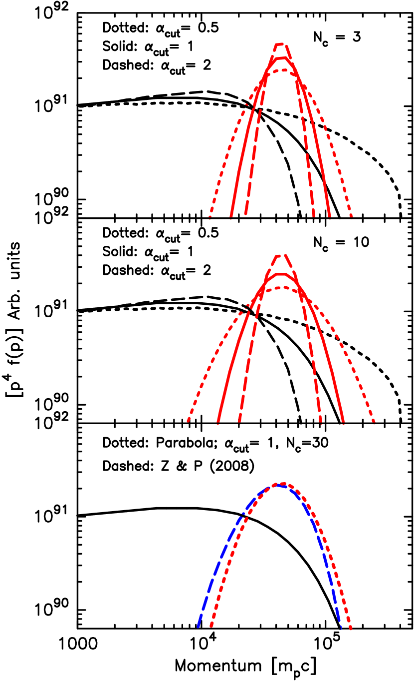
Figure 2.— The top two panels show trapped (black curves) and escaping CR (red curves) proton distributions for simulations where $\alpha_{\mathrm{cut}}$ and $N_{c}$ have been varied. The distributions are summed at the end of the simulation at $t_{\mathrm{SNR}}=1000$ yr and the escaping CR distributions are those leaving the FS before any propagation occurs. In the bottom panel we compare our parabola fit with $\alpha_{\mathrm{cut}}=1$ and $N_{c}=30$ (red dotted curve) to the result from Zirakashvili & Ptuskin (2008) (blue dashed curve). Both curves have been normalized to the total energy in escaping CRs.

Our scheme for determining $p_{\mathrm{max}}$ gives a very different result from the parameterization used in Gabici, Aharonian & Casanova (2009), as indicated in the bottom panel of Fig. 1. Gabici, Aharonian & Casanova (2009) argue that magnetic field amplification (MFA) may contribute to a strong decrease in $p_{\mathrm{max}}$ as a function of time since it might be expected that MFA is strongest at early times, yielding a large magnetic field and a higher $p_{\mathrm{max}}$. As the remnant ages, MFA might decrease, producing a stronger time dependence than the standard SNR evolution would suggest. Magnetic field amplification is not include in the examples we show here. We caution, however, that nonlinear feedback may reduce the full effects of MFA (e.g., Vladimirov, Bykov & Ellison, 2008; Caprioli et al., 2008, 2009) and we feel it is unlikely that a time dependence as strong as assumed by Gabici, Aharonian & Casanova (2009) will be obtained. In any case, our main purpose here is to introduce a new propagation tool for escaping CRs and not be overly concerned with details that are still subject to active research.

An approximate expression for the CRs that remain trapped within the SNR is (e.g., Ellison, Decourchelle & Ballet, 2005)

$$f_{\mathrm{trap}}(p)\sim f_{\mathrm{SA}}(p)\exp{\left[-\left(\frac{p}{p_{\mathrm{max}}}\right)^{\alpha_{\mathrm{cut}}}\right]}\ ,$$ (2)

where $f_{\mathrm{SA}}\sim(p/p_{\mathrm{max}})^{-4}$ is the quasi-power law DSA distribution obtained by the standard semi-analytic model, $\alpha_{\mathrm{cut}}$ is an arbitrary parameter that determines the turnover around $p_{\mathrm{max}}$, and $p_{\mathrm{max}}$, as mentioned, is determined by the SNR dynamics and $f_{\mathrm{sk}}$. The distribution of escaping CRs, $F_{\mathrm{esc}}(p)$, is parameterized by assuming that it is a parabola in $\log{(p^{4}F_{\mathrm{esc}}})$ space, that is,

$$\log{\left[(p^{\prime})^{4}F_{\mathrm{esc}}(p)\right]}=$$

$$-a\left[\log{(p^{\prime})}-\log{(1)}\right]^{2}+b\ ,$$ (3)

where $p^{\prime}=p/p_{\mathrm{max}}$. Initially, we determine $b$ such that

$$f_{\mathrm{trap}}(p_{\mathrm{max}})=F_{\mathrm{esc}}(p_{\mathrm{max}})\ ,$$ (4)

which yields $b=\log(e^{-1})=-0.434$.

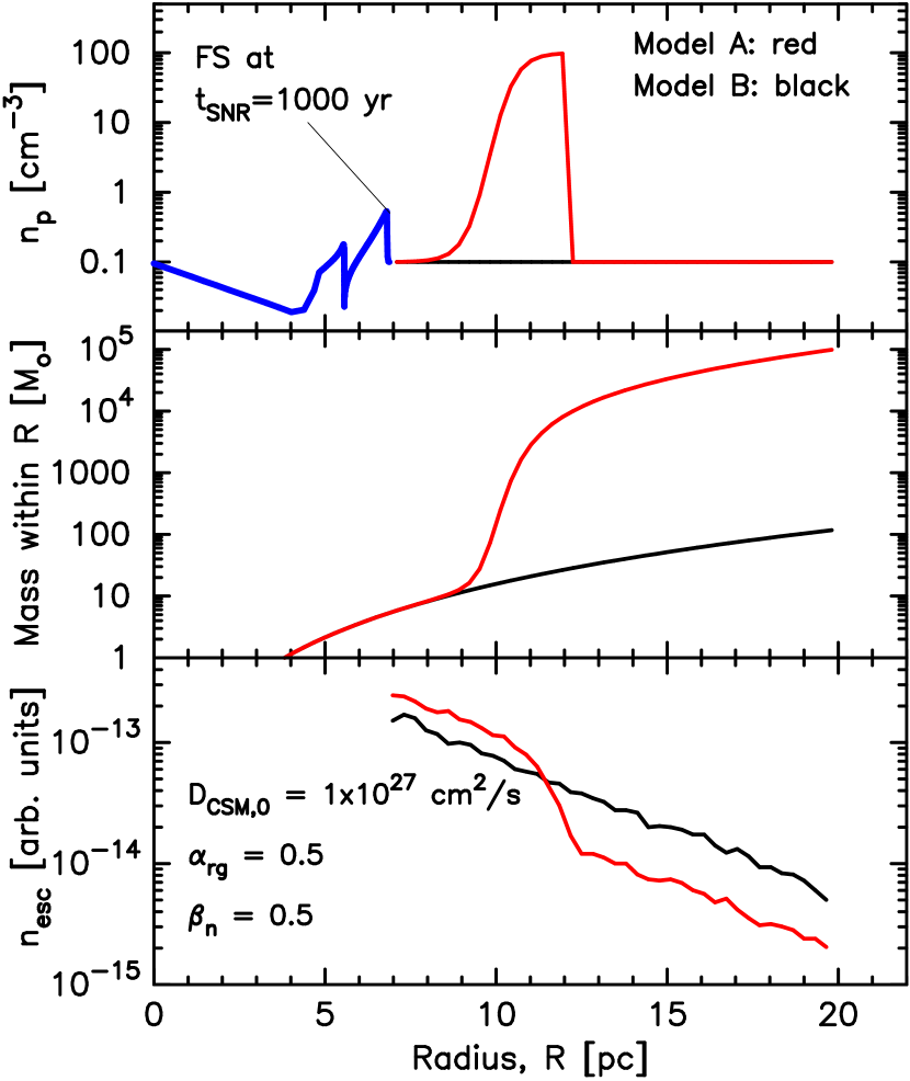
Figure 3.— The black and red curves in the top panel show two spherically symmetric CSM density profiles. The blue curve in the top panel shows the density of the SNR at $t_{\mathrm{SNR}}=1000$ yr. The two curves in the middle panel show the total mass within a particular radius for the CSM profiles at the start of the simulation. The dense shell has a mass of $M_{\mathrm{tot}}=10^{4}\,\mathrm{M}_{\odot}$. In both cases, CRs escaping from the FS of the SNR propagate in the CSM profiles and, at $t_{\mathrm{SNR}}=1000$ yr, have the color-coordinated density profiles shown in the bottom panel. The parameters for the CSM propagation (e.g., Eq. 8) are shown in the bottom panel. The density profiles shown in the bottom panel are for a particular momentum near the peak of the escaping CR distribution. The irregular variations in the escaping CR densities are a result of the stochastic nature of the Monte Carlo propagation.

The width of the parabola, $a$, is matched to $f_{\mathrm{trap}}(p)$ as follows. We determine the momentum $p_{c}>p_{\mathrm{max}}$ where the trapped CR distribution drops by some factor, $1/N_{c}$, below its value at $p_{\mathrm{max}}$, i.e.,

$$\frac{f_{\mathrm{trap}}(p_{c})}{f_{\mathrm{trap}}(p_{\mathrm{max}})}=1/N_{c}\ .$$ (5)

Specifying $N_{c}$ uniquely determines $p_{c}$. We then obtain $a$ by setting:

$$\frac{F_{\mathrm{esc}}(p_{c})}{F_{\mathrm{esc}}(p_{\mathrm{max}})}=N_{c}\ ,$$ (6)

that is,

$$a(\alpha_{\mathrm{cut}})=-\log{\left[(p^{\prime}_{c})^{4}N_{c}\right]}/\left[(\log{p^{\prime}_{c}})\right]^{2}\ ,$$ (7)

where $p^{\prime}_{c}=p_{c}/p_{\mathrm{max}}$ and we have written $a(\alpha_{\mathrm{cut}})$ to emphasize that the width of the escaping distribution depends on the cutoff parameter in the trapped CR distribution. The final normalization for $F_{\mathrm{esc}}$ is set by the total energy in the escaping distribution, $Q_{\mathrm{esc}}$, which is an output of the semi-analytic DSA model.

In the top two panels of Fig. 2 we show examples where $\alpha_{\mathrm{cut}}$ is varied between 0.5 and 2 with $N_{c}=3$ and $10$. All other parameters of the CR-hydro model are the same for these examples. In all panels, the black curves are the CRs that remain trapped in the SNR, $f(p)$, and these distributions, unlike the escaping CRs, have undergone adiabatic losses during the $t_{\mathrm{SNR}}=1000$ yr age of the remnant. The parameters, $\alpha_{\mathrm{cut}}$ and $N_{c}$ allow a fairly wide range of shapes in the critical region around $p_{\mathrm{max}}$, although it is important to note that, in our model, for all reasonable values of $\alpha_{\mathrm{cut}}$ and $N_{c}$, the escaping CR distribution is expected to be narrow compared to the trapped CRs. This differs from the work of Gabici, Aharonian & Casanova (2009), as mentioned above, and of Ohira, Murase & Yamazaki (2010) who assume a power-law form for the escaping CR distribution.

In the bottom panel of Fig. 2 we compare our parameterization (red dotted curve) using $\alpha_{\mathrm{cut}}=1$ and $N_{c}=30$ to the form presented in Zirakashvili & Ptuskin (2008) (blue dashed curve). Other than a slight offset of the peak, this choice of $\alpha_{\mathrm{cut}}$ and $N_{c}$ matches the Zirakashvili & Ptuskin (2008) result quite well. We could have obtained an equally good match with a different combination of $\alpha_{\mathrm{cut}}$ and $N_{c}$. The quality of this match with $\alpha_{\mathrm{cut}}=1$ leads us to fix $N_{c}=30$ and leave $\alpha_{\mathrm{cut}}$ as a single free parameter for the coupled shapes of the cutoff in the trapped CRs and the escaping distribution.

II.2. Monte Carlo Model of Cosmic Ray Propagation

Given the form for the escaping distribution, we propagate the escaping CRs using a Monte Carlo technique. As the CR-hydro simulation evolves, $F_{\mathrm{esc}}(p)$ is calculated for spherical shells at time-steps, $\Delta t$, as the forward shock overtakes fresh circumstellar material. As the outer-most shell is formed, escaping CRs leave the shell and diffuse into the CSM with a momentum and density dependent mean free path given by

$$\lambda_{\mathrm{CSM}}=\lambda_{\mathrm{CSM,0}}(r_{g}/r_{g,0})^{\alpha_{\mathrm{rg}}}(n_{\mathrm{CSM}}/n_{0})^{-\beta_{n}}\ .$$ (8)

Here, $r_{g}=pc/(eB)$ is the gyroradius, $n_{\mathrm{CSM}}$ is the CSM proton number density, and ${\alpha_{\mathrm{rg}}}$ and $\beta_{n}$ are parameters. For scaling, we use $n_{0}=1$ cm^-3, $r_{g,0}=10\mathrm{GeV}/(eB_{\mathrm{CSM,0}})$, and $B_{\mathrm{CSM,0}}=3$ $\mu$G. The normalization of the CSM diffusion coefficient, $D_{\mathrm{CSM,0}}=\lambda_{\mathrm{CSM,0}}\,c/3$, can be estimated from CR propagation studies (see, for example, Ptuskin et al., 2006; Gabici, Aharonian & Casanova, 2009). For example, with $D_{\mathrm{CSM,0}}=10^{27}\,$cm² s^-1, $n_{\mathrm{CSM}}=0.01$ cm^-3, ${\alpha_{\mathrm{rg}}}=0.5$, and $\beta_{n}=1$, $\lambda_{\mathrm{CSM}}\sim 1$ pc at 1 GeV, consistent with the fits of Ptuskin et al. (2006).

We note that the CSM diffusion resulting from Eq. (8) is very different from the diffusion we assume to occur within the SNR. For the acceleration process at the FS, we assume Bohm diffusion with $\lambda\sim r_{g}$. Once the trapped CRs have been accelerated in the outer shell, these CRs are assumed to remain in the shell as it convects and evolves within the remnant. In all cases, the CSM scattering is much weaker than within the SNR and the escaping CRs quickly fill the CSM out to the end of the simulation box.

The process continues until $t_{\mathrm{SNR}}$ is reached during which time some number of CR filled shells have been formed within the SNR. The escaping CRs fill the CSM region with a distribution that depends on Eq. (8) and the properties assigned to the CSM.

II.3. Circumstellar Medium Properties

We model the spherically symmetric CSM with a dense shell sitting on a low-density, uniform background of density $n_{\mathrm{uni}}$. The shell has a maximum density $n_{\mathrm{shell}}$ and an inner radius $R_{\mathrm{shell}}$ which, for the examples in this paper, is greater than the outer radius of the SNR at $t_{\mathrm{SNR}}$, that is, the blast wave of the SNR has not yet reached the dense shell at the end of the simulation. An additional parameter is the total mass in the shell, $M_{\mathrm{shell}}$.

The red curves in the top two panels of Fig. 3 show the density and mass distribution for a CSM with $n_{\mathrm{uni}}=0.1$ cm^-3, $n_{\mathrm{shell}}=100$ cm^-3, $R_{\mathrm{shell}}\sim 10$ pc, and $M_{\mathrm{shell}}=10^{4}\,\mathrm{M}_{\odot}$. Note that the dense shell smoothly rises from $n_{\mathrm{uni}}=0.1$ cm^-3 and the rise is centered on $R_{\mathrm{shell}}$. The black curves show the CSM with no shell. The total extent of the simulation box for these examples is $\sim 20$ pc. Also shown in the top panel (blue curve) is the density profile of the SNR at the end of the simulation, i.e., at $t_{\mathrm{SNR}}=1000$ yr. The FS, contact discontinuity, and RS can be easily discerned from the figure.

The addition of the escaping CR distribution requires additional parameters and Table 1 gives the parameters for the CSM diffusion and the parameters for the external medium. As mentioned above, we restrict ourselves to a spherically symmetric CSM in this first presentation of the Monte Carlo propagation model.

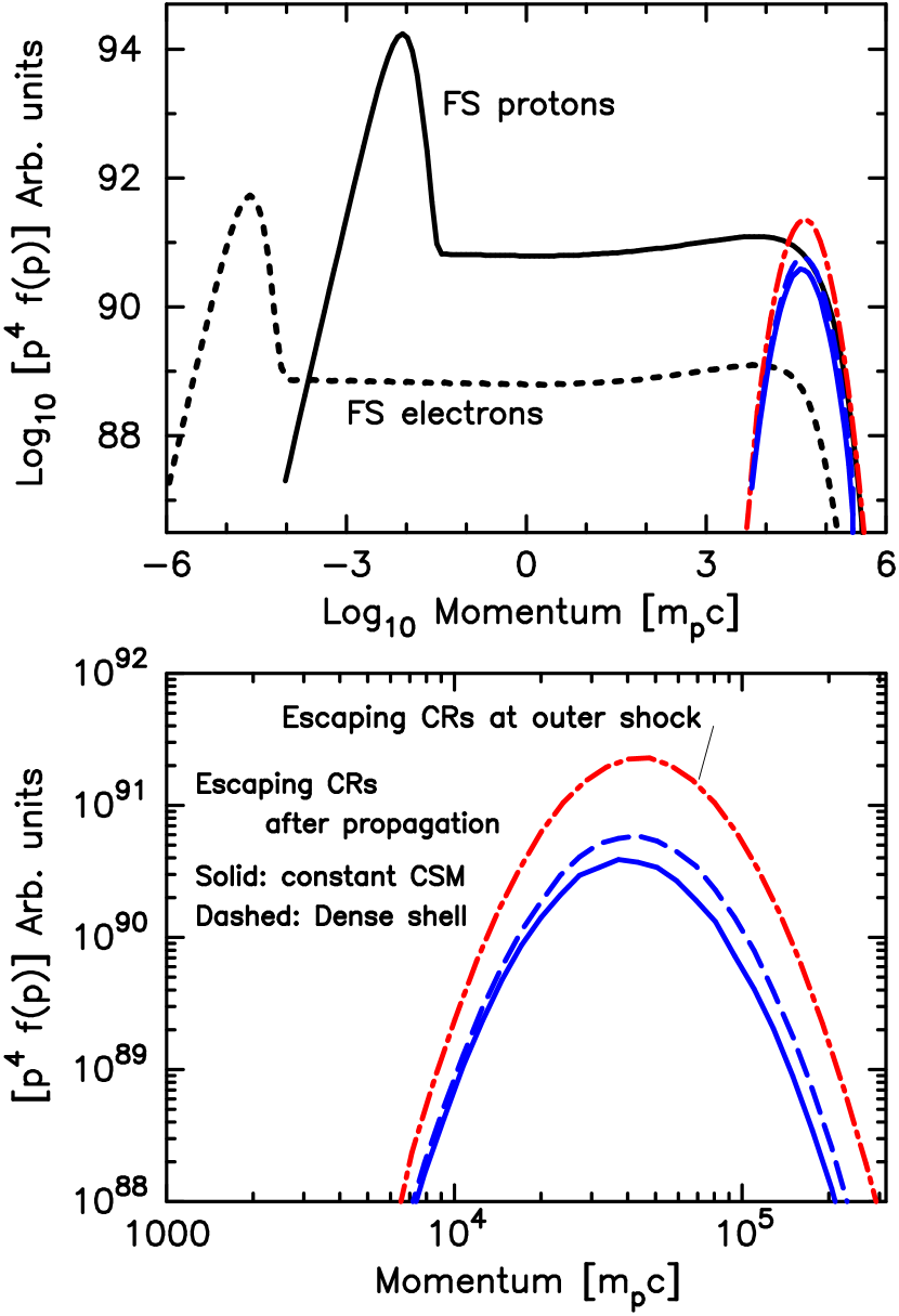
Figure 4.— The top panel shows the total CR spectra within the forward shock at $t_{\mathrm{SNR}}=1000$ yr (black solid curve: protons; black dotted curve: electrons), along with the escaping CRs. The red curves in both panels show the escaping CR distribution at the FS, while the blue solid and dashed curves show the escaping CRs after diffusing in the CSM profiles shown in Fig. 3. The solid blue curves (Model B) are for the constant CSM and the dashed blue curves (Model A) are for the dense shell. The two models in this plot have ${\alpha_{\mathrm{rg}}}=\beta_{n}=0.5$ and $D_{\mathrm{CSM,0}}=1\!\times\!10^{27}$ cm²/s.

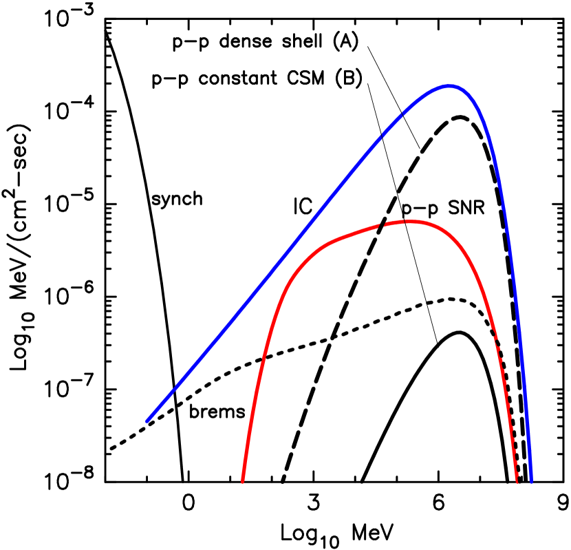
Figure 5.— Photon spectra at Earth for the examples shown in Fig. 4. As expected, the case with a dense external shell (Model A) shines much more brightly in $\gamma$-rays than the case with a low density, uniform external CSM (Model B). The individual components for synchrotron, inverse-Compton, bremsstrahlung, and the pion-decay emission from CRs that remain trapped in the SNR are indicated.

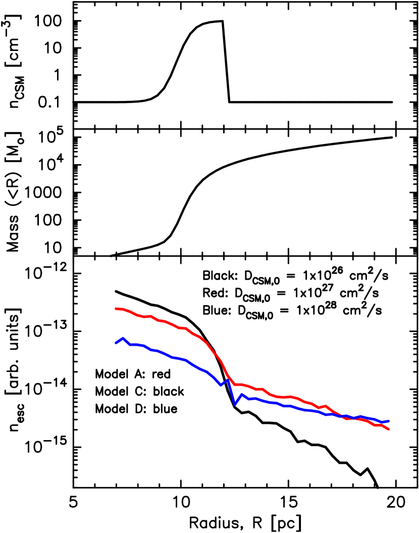
Figure 6.— Escaping CR diffusion in a dense external shell as a function of the normalization of $D_{\mathrm{CSM}}$. In all cases, ${\alpha_{\mathrm{rg}}}=\beta_{n}=0.5$.

III. Results

We use the following environmental parameters for all of our examples: (i) the SN explosion energy, $E_{\mathrm{SN}}=10^{51}$ erg; (ii) the ejecta mass, $M_{\mathrm{ej}}=1.4\,\mathrm{M}_{\odot}$; (iii) the distance to the SNR, $d_{\mathrm{SNR}}=1$ kpc, and; (iv) the ambient magnetic field throughout the CSM, $B_{\mathrm{CSM}}=3$ $\mu$G.

For the diffusive shock acceleration of trapped and escaping CRs, we fix the following: (i) the fraction of FS radius used to determine $p_{\mathrm{max}}$, $f_{\mathrm{sk}}=0.1$; (ii) the magnetic field amplification factor, $B_{\mathrm{amp}}=1$, i.e., no MFA is used; (iii) the matching factor defined in equation (5), $N_{c}=30$, and; (iv) the DSA efficiency, ${\cal E_{\mathrm{DSA}}}=50$%.

The parameters for DSA and the CSM propagation that are varied for our examples are given in Table 1. Again we note that we are not attempting a detailed fit to any particular remnant and that our model is not restricted to the particular values for parameters we use here. Any of the environmental or DSA parameters can be modified to match a specific object.

In Fig. 3 we show results for Models A (with a dense external shell) and B (no external shell), as listed in Table 1. The top two panels were discussed in Section II.3. In the bottom panel of Fig. 3 we show the escaping CR densities at $t_{\mathrm{SNR}}=1000$ yr. The escaping densities shown are for a single momentum near the peak of $F_{\mathrm{esc}}$ and the parameters assumed for the CSM propagation are noted in the figure. The escaping CRs are emitted from the SNR as it evolves so the escaping CRs that were produced earliest have been diffusing for approximately $t_{\mathrm{SNR}}=1000$ yr and many have left the simulation box.

For the case where the CSM is uniform (black curves), the escaping CRs diffuse outward and uniformly fill the region beyond the SNR forward shock with a density that deceases uniformly with radius as expected. With the dense shell, the escaping CR density drops rapidly as the CRs enter the shell. With this $M_{\mathrm{shell}}=10^{4}\,\mathrm{M}_{\odot}$, the shell is about 2 pc thick. Cosmic rays that propagate beyond $R_{\mathrm{max}}\sim 20$ pc are removed from the simulation.

In the top panel of Fig. 4 we show the CR distributions for both the CRs that remain trapped in the SNR (black solid and dotted curves) and escaping CRs. In all cases, the integrated distributions are determined at $t_{\mathrm{SNR}}=1000$ yr. The red curve in the top panel is the summed escaping distribution as the CRs leave the FS, i.e., before they propagate into the external CSM. The solid and dashed blue curves are the escaping CRs, at $t_{\mathrm{SNR}}=1000$ yr, after propagation and we remind the reader that our escaping CR fluxes are over estimates since we don’t model dilution which, in fact, occurs simultaneously with escape. The bottom panel shows just the escaping CRs with an expanded scale. Note that throughout this paper we include only escaping protons and ignore escaping heavier ions and escaping electrons. Trapped electrons are considered for inverse-Compton emission. The distributions for the escaping CRs after propagation are lower than the distribution as CRs leave the FS for two reasons. The first is that some CRs escape from the simulation box at $R_{\mathrm{max}}$. The second is that some escaping CRs diffuse back into the SNR and these CRs are ignored and not included in the blue distributions in Fig. 4. The CRs that remain trapped in the shock are summed from the contact discontinuity to the forward shock.

In Fig. 5 we show the various photon components for the models with ${\alpha_{\mathrm{rg}}}=\beta_{n}=0.5$ and $D_{\mathrm{CSM,0}}=1\!\times\!10^{27}$ cm²/s. The results for the two models are identical except for the pion-decay emission from the escaping CRs. As expected, escaping CRs interacting with the dense external shell produce substantially more emission than those interacting with the uniform CSM. In both cases, however, the emission from escaping CRs is much more strongly peaked than the pion-decay emission from the trapped CR protons. For the trapped CRs, the relative intensity of the pion-decay emission and the inverse-Compton emission depends on the various parameters chosen, most particularly $n_{\mathrm{uni}}$ and $K_{\mathrm{ep}}$, the electron to proton ratio at relativistic energies. The fact that our values, $n_{\mathrm{uni}}=0.1$ cm^-3 and $K_{\mathrm{ep}}=0.01$, result in inverse-Compton dominating the GeV-TeV emission is not necessarily an indication that we believe this will always be the case. The issue is more complicated as indicated in a number of recent papers (see, for example, Katz & Waxman, 2008; Morlino, Amato & Blasi, 2008; Zirakashvili & Aharonian, 2010; Ellison et al., 2010). Regardless of other parameters, the relative importance of the $\gamma$-ray emission from escaping CRs and trapped CRs depends mainly on the external density enhancement.

In Fig. 6 we show the effect of the normalization of the CSM diffusion coefficient as escaping CRs diffuse into the dense shell. Three effects are noticeable. The first is that the escaping CR density drops more rapidly with stronger scattering (i.e., smaller $D_{\mathrm{CSM,0}}$) as CRs enter the dense shell. The second is that the escaping CR density remains larger in the region between the FS and the dense shell when scattering is strong even though the flux of escaping CRs that leave the FS is the same in all three cases. The third effect is that, beyond the dense shell, the escaping CR density falls off faster with stronger scattering. The CR density remains large within the shell (i.e., at radii $\lesssim 10$ pc) for strong scattering because the dense shell acts as a valve that slows the flow of CRs out of the system. Beyond the dense shell, weak scattering results in a more uniform density distribution than strong scattering since CRs rapidly fill the available volume when the scattering is weak.

In Fig. 7 we compare the pion-decay emission for the three examples given in Fig. 6, all with the same ambient density distribution. The CRs trapped in the SNR are the same for these cases so the pion-decay emission from the trapped CRs (dashed curve) is the same in the three models. Also identical for the three cases is the escaping CR flux as it emerges from the FS. The sole difference is the scattering strength, $D_{\mathrm{CSM,0}}$, in the CSM and this produces a fairly strong effect on the pion-decay emission from the escaping CRs. While the emission from escaping CRs shown in Figs. 5 and 7 is summed over the entire region from the outer radius of the SNR at $t_{\mathrm{SNR}}$ to $R_{\mathrm{max}}\sim 20$ pc, when a dense shell is present, most of the emission originates in the shell, as expected.

In Fig. 8 we compare escaping CR distributions for different power-law dependences of the gyroradius, i.e., ${\alpha_{\mathrm{rg}}}=1/3$ (Model E), ${\alpha_{\mathrm{rg}}}=1/2$ (Model F), and ${\alpha_{\mathrm{rg}}}=1$ (Model G). For variety, the models in Fig. 8, along with those in Fig. 9 below, use a different set of CSM parameters than the models discussed thus far, as shown in Table 1. For the three examples shown, the CSM parameters are identical and the mean free paths differ only in the value of ${\alpha_{\mathrm{rg}}}$; the normalization of the diffusion coefficient $D_{\mathrm{CSM,0}}=10\!\times\!10^{27}$ cm² s^-1 and $\beta_{n}=0.5$ are the same for the three values of ${\alpha_{\mathrm{rg}}}$. As the dependence on ${\alpha_{\mathrm{rg}}}$ increases, the high momentum CRs are able to stream through the CSM quickly and the number that remain within the simulation region at $t_{\mathrm{SNR}}=1000$ yr drops. The strong ${\alpha_{\mathrm{rg}}}$ dependence also results in a flatter radial density distribution, as indicated by the blue curve in the bottom panel of Fig. 8. The reason for this is that the momentum near the peak in the escaping distribution that is used to calculate the density profiles is well above 10 GeV so the examples with larger ${\alpha_{\mathrm{rg}}}$ have longer mean free paths.

In Fig. 9 we show a similar plot where we now keep ${\alpha_{\mathrm{rg}}}=0.5$ and vary the power-law index for the density dependence of the diffusion coefficient, $\beta_{n}$. When $\beta_{n}=0$ and there is no density dependence for the diffusion coefficient, the presence of the external dense shell produces no effect and the red curve in the bottom panel of Fig. 9 falls off uniformly with radius. For stronger density dependences (green and blue curves), the density of escaping CRs drops as they enter the dense external shell which has a radius $R_{\mathrm{shell}}\simeq 7$ pc for these models and those shown in Fig.  8.

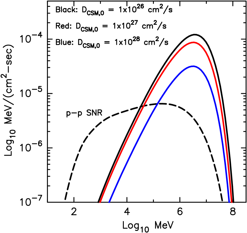
Figure 7.— Gamma-ray emission for the three cases shown in Fig. 6. Since only the interaction of escaping CRs with the external CSM is varied, the pion-decay emission from the trapped CRs within the SNR is the same for the three cases. Referring to Table 1, the black solid curve is Model C, the red solid curve is Model A, and the blue solid curve is Model D.

In Figs. 10 and 11 we compare pion-decay emission for $\alpha_{\mathrm{cut}}=1/2$ (Model J) and $\alpha_{\mathrm{cut}}=2$ (Model K). All other parameters for these two models are the same as indicated in Table 1. As seen in the top panels of these figures, the CR distributions vary considerably for these values of $\alpha_{\mathrm{cut}}$. The photon emission (bottom panels), of the trapped (dashed curves) and escaping CRs (solid curves) varies less strongly due to the fact that the photon emission is naturally spread out partially masking the shape of the underlying proton spectrum. One clear feature that remains is the low-energy kinematic cutoff at a few hundred MeV. Of course, Figs. 10 and 11 were calculated for a particular set of parameters and the relative importance of photon emission from escaping CRs versus trapped CRs will depend strongly on these parameters.

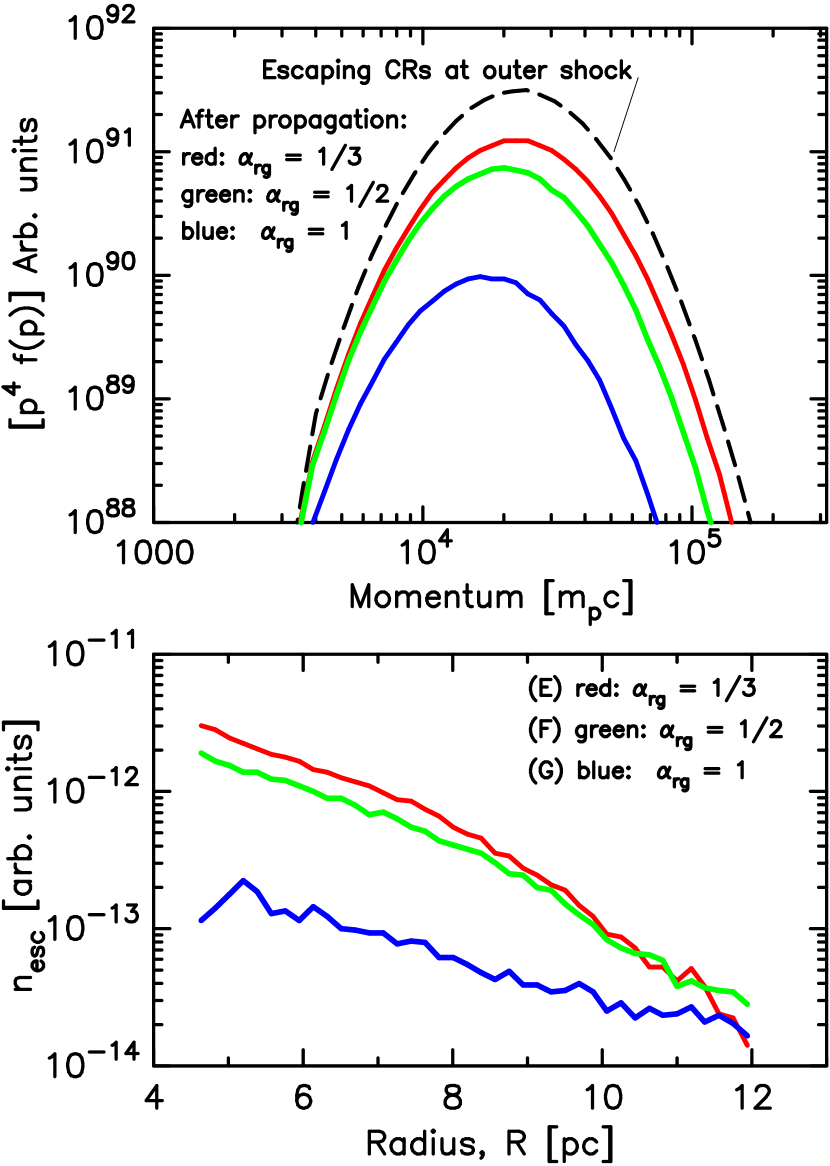
Figure 8.— Escaping CR distributions, $F_{\mathrm{esc}}$, (top panel), and density profiles (bottom panel) for Models E, F, and G, as listed in Table 1. The index ${\alpha_{\mathrm{rg}}}$ is varied as shown and $\beta_{n}=0.5$ in all cases. For these examples, and those shown in Fig. 9, $n_{\mathrm{uni}}=1$ cm^-3, $n_{\mathrm{shell}}=10$ cm^-3, $R_{\mathrm{shell}}=7$ pc, and the densities in the bottom panel are for a particular momentum near the peak of the escaping CR distribution. The simulation box extends to 12 pc.

IV. Discussion and Conclusions

As part of a comprehensive model of an evolving SNR undergoing efficient CR production, we have presented a Monte Carlo technique that describes the diffusion of CRs that escape from the forward shock of the remnant and propagate into a dense, external shell. While a number of calculations of escaping CRs and their $\gamma$-ray production have been performed (see, for example, Lee, Kamae & Ellison, 2008; Ohira, Murase & Yamazaki, 2010; Drury, 2010, and references therein), there remain many unresolved issues for this important problem. Our Monte Carlo method makes different assumptions than analytic calculations based on solving a diffusion equation and in some ways is less restrictive, particularly if energy losses are included during propagation.

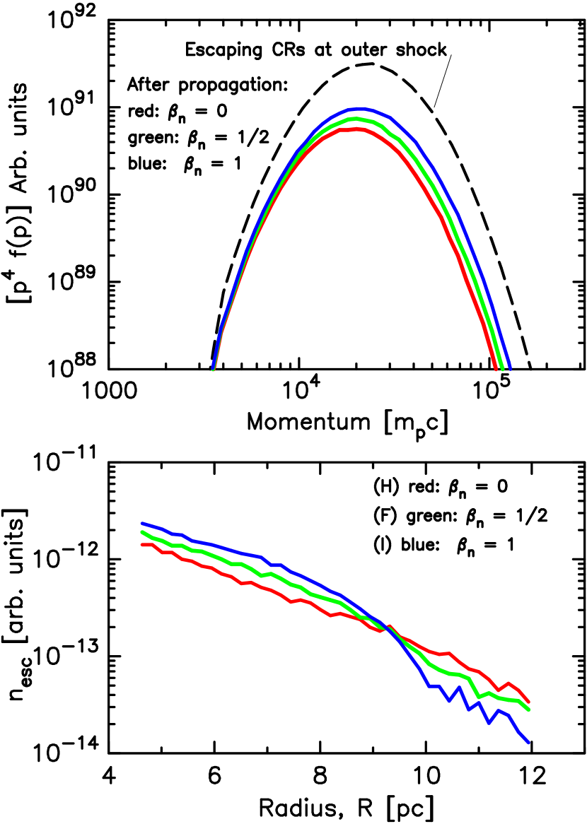
Figure 9.— Escaping CR distributions, $F_{\mathrm{esc}}$, (top panel), and density profiles (bottom panel) for Models H, F, and I, as listed in Table 1. Note that the green curves (Model F) are identical in Figs. 8 and 9. The index $\beta_{n}$ is varied as shown and ${\alpha_{\mathrm{rg}}}=0.5$ in all cases.

Figure 10.— The top panel shows particle spectra for trapped CRs (dashed curve) and escaping CRs (solid curve). The bottom panel shows the corresponding pion-decay emission for these distributions along with the sum (dotted curve).

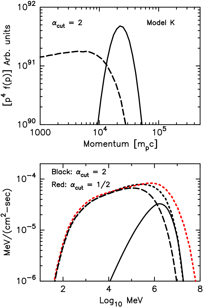
Figure 11.— Same as in Fig. 10 with $\alpha_{\mathrm{cut}}=2$. In the bottom panel we compare the summed emission for the two cases $\alpha_{\mathrm{cut}}=1/2$ (red dotted curve) and $\alpha_{\mathrm{cut}}=2$ (black dotted curve).

The important features of our model include: (i) the energy content of the escaping CR distribution is determined with the shock accelerated CRs that remain trapped within the SNR using a planar, stationary, nonlinear model of efficient diffusive shock acceleration that neglects dilution (i.e., Blasi, Gabici & Vannoni, 2005); (ii) the acceleration of CRs produces changes in the hydrodynamics that modifies the evolution of the SNR; (iii) the shape of the trapped CR distribution at the highest energies, which is uncertain due to a lack of a well developed theory of turbulence generation for anisotropic particles, is parameterized consistently with the shape of the escaping CR distribution; (iv) the broad-band continuum photon emission from escaping and trapped CRs is determined with a single set of environmental and model parameters; and (v) although not emphasized or shown in the plots here, the thermal X-ray emission is included consistently with the broad-band continuum emission (e.g., Ellison et al., 2010, and references therein).

The examples we show indicate the complexity and importance of including escaping CRs in a consistent fashion with CRs that remain trapped within the SNR. The shape of the GeV-TeV emission, particularly the low-energy kinematic cutoff, is important as one of the main ways of determining whether this emission is pion-decay or inverse-Compton. If other features are discernable, they may provide clues to the importance of the escaping CRs and external density enhancements. We note that all of the spectra shown here are integrated over the region between the contact discontinuity and the forward shock and are not line-of-sight projections. It should be clear from Fig. 6 that line-of-sight projections might show additional strong effects as escaping CRs interact with nearby dense material. Line-of-sight projections will be included in future work.

An important parameter that we haven’t varied here is the efficiency of DSA. In all of our examples we set ${\cal E_{\mathrm{DSA}}}=50$%, i.e., 50% of the forward shock ram kinetic energy flux goes into CRs (trapped and escaping) at any instant. In fitting an actual SNR, ${\cal E_{\mathrm{DSA}}}$ is a parameter that may or may not be constrained by the observations. A considerable amount of work has led to the conclusion that ${\cal E_{\mathrm{DSA}}}\sim 50$% is a likely figure for young SNRs but this efficiency will definitely vary between remnants, may vary during the remnant lifetime, and may even vary at different locations in a single SNR (see, for example, Völk, Berezhko & Ksenofontov, 2003). We note that Monte Carlo shock simulations that include MFA and have parameters typical of young SNRs (e.g., Vladimirov, Ellison & Bykov, 2006; Vladimirov, Bykov & Ellison, 2008), show total acceleration efficiencies ${\cal E_{\mathrm{DSA}}}\geq 50$% with a sizable fraction of total shock ram kinetic energy ($\geq 30$%) placed in escaping CRs.

Since we set ${\cal E_{\mathrm{DSA}}}=50$% for all of our examples, and the other SNR parameters that determine what fraction of explosion energy ends up in CRs are kept constant, the third panel in Fig. 1 gives the results for all of our models. After 1000 yr, $\sim 30$% of the supernova explosion energy has gone into all CRs with $\sim 10$% going into escaping CRs. At 10,000 yr, $\sim 50$% has gone into all CRs with $\sim 20$% going into escaping CRs.

In this initial presentation of our Monte Carlo technique, we have exploded the supernova in a uniform CSM with an external, spherically symmetric shell of dense material. This simple scenario shows how important escaping CRs can be for modeling non-thermal emission of young SNRs. It is not meant to match any particular object. The Monte Carlo propagation part of the CR-hydro model can be easily generalized to include asymmetric external mass distributions, such as those expected when remnants interact with a dense molecular cloud (e.g., SNR RX J1713.7-3946). Future work will also model $\gamma$-rays produced when escaping CRs interact with the complex structure of a dense surrounding shell as expected from a progenitor stellar wind.

Table 1Parameters for DSA and circumstellar medium diffusion.

Model	$K_{\mathrm{ep}}$	$\alpha_{\mathrm{cut}}$	$D_{\mathrm{CSM,0}}$	$\lambda_{\mathrm{CSM,0}}$	${\alpha_{\mathrm{rg}}}$	$\beta_{n}$	$n_{\mathrm{uni}}$	$n_{\mathrm{shell}}$	$M_{\mathrm{shell}}$	$R_{\mathrm{shell}}$
			[cm2s-1]	[pc]			[cm-3]	[cm-3]	[$\mathrm{M}_{\odot}$]	[pc]
A	$1\!\times\!10^{-2}$	1	$1\!\times\!10^{27}$	$3.3\!\times\!10^{-2}$	0.5	0.5	0.1	100	$10^{4}$	10
B	$1\!\times\!10^{-2}$	1	$1\!\times\!10^{27}$	$3.3\!\times\!10^{-2}$	0.5	0.5	0.1	—	—	—
C	$1\!\times\!10^{-2}$	1	$1\!\times\!10^{26}$	$3.3\!\times\!10^{-3}$	0.5	0.5	0.1	100	$10^{4}$	10
D	$1\!\times\!10^{-2}$	1	$1\!\times\!10^{28}$	$3.3\!\times\!10^{-1}$	0.5	0.5	0.1	100	$10^{4}$	10
E	$1\!\times\!10^{-2}$	1	$1\!\times\!10^{27}$	$3.3\!\times\!10^{-2}$	1/3	0.5	1	10	$10^{3}$	7
F	$1\!\times\!10^{-2}$	1	$1\!\times\!10^{27}$	$3.3\!\times\!10^{-2}$	0.5	0.5	1	10	$10^{3}$	7
G	$1\!\times\!10^{-2}$	1	$1\!\times\!10^{27}$	$3.3\!\times\!10^{-2}$	1	0.5	1	10	$10^{3}$	7
H	$1\!\times\!10^{-2}$	1	$1\!\times\!10^{27}$	$3.3\!\times\!10^{-2}$	0.5	0	1	10	$10^{3}$	7
I	$1\!\times\!10^{-2}$	1	$1\!\times\!10^{27}$	$3.3\!\times\!10^{-2}$	0.5	1	1	10	$10^{3}$	7
J	$1\!\times\!10^{-4}$	0.5	$1\!\times\!10^{27}$	$3.3\!\times\!10^{-2}$	0.5	0.5	1	10	$10^{3}$	7
K	$1\!\times\!10^{-4}$	2	$1\!\times\!10^{27}$	$3.3\!\times\!10^{-2}$	0.5	0.5	1	10	$10^{3}$	7