Molecular investigations of comets C/2002 X5 (Kudo-Fujikawa), C/2002 V1 (NEAT), and C/2006 P1 (McNaught) at small heliocentric distances

We present unique spectroscopic radio observations of comets C/2002 X5 (Kudo-Fujikawa), C/2002 V1 (NEAT), and C/2006 P1 (McNaught), which came within $r_{h}\approx$ 0.2 AU of the Sun in 2003 and 2007. The molecules OH, HCN, HNC, CS, and CH${}_{3}$OH were detected in each of these comets when they were exposed to strong heating from the Sun. Both HC${}_{3}$N and HCO${}^{+}$ were detected in comets C/2002 X5 and C/2006 P1, respectively. We show that in these very productive comets close to the Sun screening of the photodissociation by the Sun UV radiation plays a non-negligible role. Acceleration of the gas expansion velocity and day-night asymmetry is also measured and modeled. The CS photodissociation lifetime was constrained to be about $2.5\times 10^{-5}$ s${}^{-1}$ at $r_{h}=1$ AU. The relative abundances are compared to values determined from more distant observations of C/2002 X5 or other comets. A high HNC/HCN production-rate ratio, in the range 10–30% between 0.5 and 0.1 AU from the Sun, is measured. The trend for a significant enrichment in CS in cometary comae (CS/HCN$\propto r_{h}^{-0.8}$) is confirmed in all three comets. The CH${}_{3}$OH/HCN production rate ratio decreases at low $r_{h}$. The HC${}_{3}$N/HCN production rate ratio in comet C/2002 X5 is four times higher than measured in any other comet.

1 Introduction

The composition of cometary nuclei is of strong interest in understanding their origin. Having spent most of their time in a very cold environment, these objects should not have evolved much since their formation. Thus, their composition provides clues to the composition in the outer regions of the Solar Nebula where they formed. The last two decades have proven the efficiency of microwave spectroscopy in investigating the chemical composition of cometary atmospheres. About 20 different cometary molecules have now been identified at radio wavelengths (Boc04a).

In this paper, we extend our investigations of the composition of cometary atmospheres from radio observations (Boc04a; Biv02a; Biv06a; Biv07b) to three comets observed in 2003 and 2007. These observations were designed to measure the molecular abundances of comets approaching close to the Sun to investigate how the strength of the solar heating of both the comet nucleus and of its environment affects the coma composition. Previous observations have suggested that the relative production rates of several molecules vary with heliocentric distance (Biv06a). The passages of comets C/2002 X5 (Kudo-Fujikawa), C/2002 V1 (NEAT), and C/2006 P1 (McNaught) provided us with the opportunity to measure molecular abundances at heliocentric distances ($r_{h}$) between 0.1 and 0.25 AU, about one order of magnitude smaller than usual. This study is complementary to the long-term monitoring of comet C/1995 O1 (Hale-Bopp) (Biv02b), which provided information on the outgassing of a comet between 0.9 and 14 AU.

Opportunities to plan observations of comets passing within 0.2 AU from the Sun are rare. For example, comet C/1998 J1 (SOHO) was discovered too late to establish an accurate ephemeris around perihelion time. In addition, Sun-grazing comets often do not survive and even disintegrate before reaching perihelion, making observing plans extremely difficult. The last opportunity was comet C/1975 V1 (West). The observations reported here are unique, and required to develop specific observing strategies and analyses.

The organization of the paper is as follows. In Sect. 2, we present the observations of comets C/2002 X5 (Kudo-Fujikawa), C/2002 V1 (NEAT), and C/2006 P1 (McNaught) performed with the 30-m telescope of the Institut de Radioastronomie Millimétrique (IRAM) and the Nançay radio telescope. In Sects. 3 and 4, the analysis of these observations is presented. A summary follows in Sect. 5.

2 Observations

Owing to the late discovery or assessment of their activity, the three comets were observed as targets of opportunity using the IRAM 30-m and Nançay radio telescopes. This was possible because these telescopes do not have tight solar elongation constraints. The small solar elongation ($<$ 10° at $r_{h}$ $<$ 0.2 AU) resulted in limited observing support from other observatories.

Table 1: Observing conditions and ephemeris errors

Comet	UT date	$r_{h}$	$\Delta$	Phase	$O-C_{u}$${}^{\footnotesize{1}}$		$C_{f}-C_{u}$${}^{\footnotesize{1}}$
	[yyyy/mm/dd.d]	[AU]	[AU]	[${}^{\circ}$]	$\delta$RA	$\delta$Dec.	$\delta$RA	$\delta$Dec.
C/2002 X5	2003/01/13.6	0.553	1.032	69.3	-	-	+1.6″	–2.2″
	2003/01/26.5	0.214	1.172	26.1	1.5″	–11″	+0.9″	–10.3″
	2003/03/12.7	1.184	1.096	50.5	-	-	+3.0″	+0.9″
C/2002 V1	2003/02/16.6	0.135	0.978	90.3	–1.9″	–3.5″	–3.9″	–6.6″
	2003/02/17.6	0.107	0.986	87.7	–1.5″	–4.5″	–2.5″	–8.8″
C/2006 P1	2007/01/15.6	0.207	0.817	140.0	+1″	+30″	–1.2″	+27.1″
	2007/01/16.6	0.229	0.822	129.3	+1″	+28″	+0.6″	+25.7″
	2007/01/17.6	0.256	0.833	119.1	+0″	+23″	+2.0″	+23.5″

${}^{1}$ $O$, $C_{u}$, and $C_{f}$ denote the position of the HCN peak emission determined from mapping, the used computed ephemeris, and the final (reference) ephemeris, respectively. Orbital elements are given for C/2002 X5 (MPEC 2003-A41, 2003-A84, and 2003-D20 used, JPL#40${}^{2}$ reference), C/2002 V1 (MPEC 2003-C42 used, JPL#34 reference), C/2006 P1 (JPL#15, JPL#25 reference). The uncertainty in reference orbit is 2″.
${}^{2}$: JPL HORIZONS ephemerides: http://ssd.jpl.nasa.gov/?ephemerides

2.1 C/2002 X5 (Kudo-Fujikawa)

Comet C/2002 X5 (Kudo-Fujikawa) was discovered visually at $m_{v}$ = 9 on 13–14 December 2002 by two Japanese amateur astronomers, T. Kudo and S. Fujikawa (iauc8032). At about 1.2 AU from the Earth and the Sun at that time, it was then a moderately active comet. It passed perihelion on 29 January 2003 at a perihelion distance $q$ = 0.190 AU from the Sun.

One of the main goals of the observations of comet C/2002 X5 at the IRAM 30-m was to measure the evolution of the HNC/HCN production rate ratio as it approached the Sun. A first observing slot was scheduled on 4–5 January 2003, at $r_{h}$ = 0.8 AU, but the weather prevented any observation. Observations performed on 13 January ($r_{h}=0.55$ AU) only partly succeeded because of technical problems. Most data were acquired on 26.5 January, 2 days before perihelion, at $r_{h}$ = 0.21 AU. At that time, the comet was only observable visually by the C3 coronagraph aboard the SOlar Heliospheric Observatory (SOHO) — the solar elongation was 5.5°  (Bou03; Pov03). The pointing of the comet was a real challenge, since the ephemeris uncertainty was expected to be on the order of the beam size (10–20″). Since at $r_{h}$ = 0.2 AU molecular lifetimes are typically shorter than an hour, hence photodissociation scale lengths are smaller than the beam size, accurate pointing was required. From coarse mapping, we found the comet about 10″ south of its predicted position (Fig. 1, Table 1). The last observing run at IRAM took place on 12 March 2003 ($r_{h}$ = 1.2 AU, Fig. 3), when the comet was receding from the Sun and about 100 times less productive. A log of the observations and measured line areas are given in Table 2. Sample spectra are shown in Figs 2–4.

To monitor the water production rate, observations of OH at 18-cm using the Nançay radio telescope were scheduled on a daily basis from 1 January to 10 April 2003. The OH lines were only detected when the comet was between 1 and 0.4 AU from the Sun, inbound and outbound.

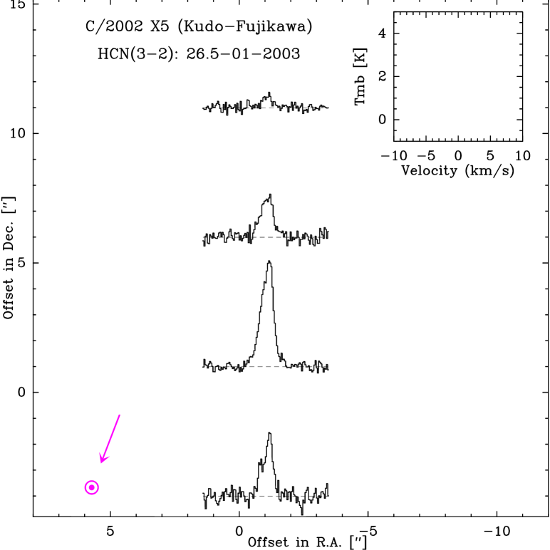
Figure 1: Coarse map of the HCN $J=$ 3–2 emission from comet C/2002 X5 (Kudo-Fujikawa) observed with the IRAM 30-m. Positional offsets in arcsec are with respect to the final ephemeris (Table 1). All four spectra are plotted at the same intensity and velocity scales, provided in the upper right box. The projected direction of the Sun is also given.

Figure 2: CH${}_{3}$OH lines at 157 GHz observed with the IRAM 30-m telescope in comet C/2002 X5 (Kudo-Fujikawa) on 26.5 January 2003. The vertical scale is main-beam brightness temperature. The horizontal scales are the rest frequency (upper scale) or the Doppler velocity in the comet rest-frame, relative to the ($6_{0}-6_{-1}$)E line frequency (bottom scale).

Figure 3: HCN $J=$ 3–2 line observed with the IRAM 30-m telescope in comet C/2002 X5 (Kudo-Fujikawa) on 12.7 March 2003. The vertical scale is the main beam brightness temperature. The horizontal scale is the Doppler velocity in the comet rest-frame.

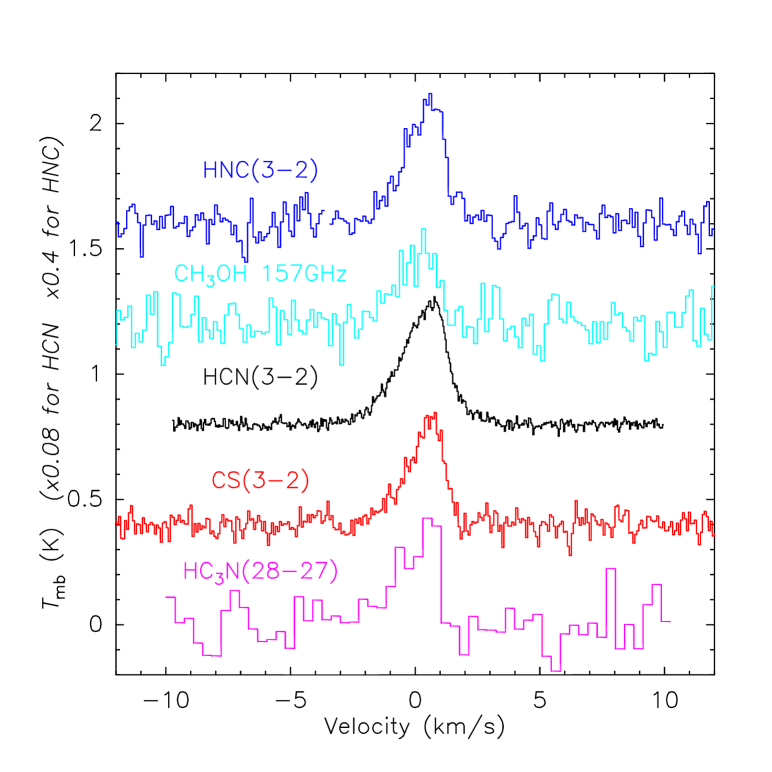
Figure 4: HC${}_{3}$N, CS, HCN, CH${}_{3}$OH (sum of the 3 brightest lines at 157 GHz) and HNC lines observed with the IRAM 30-m telescope in comet C/2002 X5 (Kudo-Fujikawa) on 26.5 January 2003. The spectra are plotted with the same horizontal scale to compare the line widths. The intensities of the spectra of HCN and HNC were divided by 12.5 and 2.5, respectively. Spectra are shifted vertically for clearer viewing.

2.2 C/2002 V1 (NEAT)

Comet C/2002 V1 (NEAT) was discovered on 6 November 2002 by the Near Earth Asteroid Tracking (NEAT) program telescope on the Haleakala summit of Maui, Hawaii (iauc8010). At that time, it was a relatively faint object ($m_{v}$ = 17). Comet C/2002 V1 (NEAT) brightened rapidly after its discovery, becoming a potentially interesting target for observations at perihelion on 18 February 2003 at $q$ = 0.099 AU. The orbital period was estimated to be 9000 years (Nakano note NK965 ), suggesting that it has survived a close passage to the Sun at its previous perihelion and might be expected to do so again.

The observations at IRAM were undertaken on 16 and 17 February 2003 ($r_{h}$ = 0.13–0.11 AU), i.e., just one day before perihelion. As for comet C/2002 X5 (Kudo-Fujikawa), the observations were challenging because of the lack of supporting optical astrometry, the comet being 8–6${}^{\circ}$ away from the Sun and only seen by the SOHO coronagraph when it became as bright as magnitudes $-1$ to $-2$. A coarse map of the HCN $J$=3–2 line at IRAM revealed the comet to be at about 5.5″ (half a beam, Fig. 5, Table 1) from its expected position. Observational data are given in Table 3.

OH 18-cm observations were obtained nearly every day from 31 December 2002 to 25 March 2003. The comet was only detected at $r_{h}>0.4$ AU from the Sun, though the water production rate ($Q_{\rm H_{2}O}$) likely exceeded $2\times 10^{30}$ molec. s${}^{-1}$ at perihelion (Sect.3).

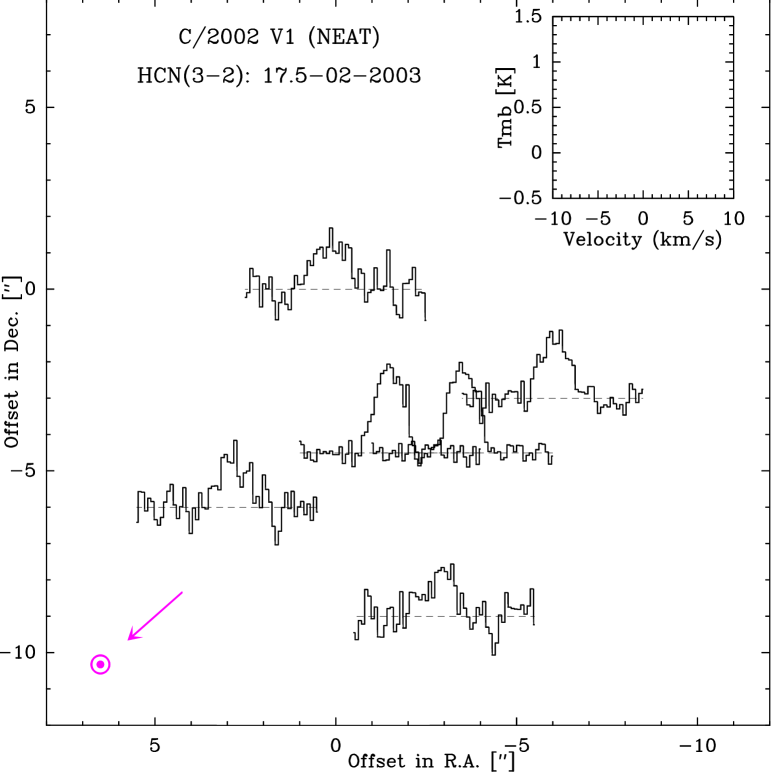
Figure 5: Scales as in Fig. 1: coarse map of the HCN $J$ = 3–2 emission in comet C/2002 V1 (NEAT) with the IRAM 30-m on 17.5 February 2003. But in this case, spectra are plotted at positions relative to the ephemerides used during the observations.

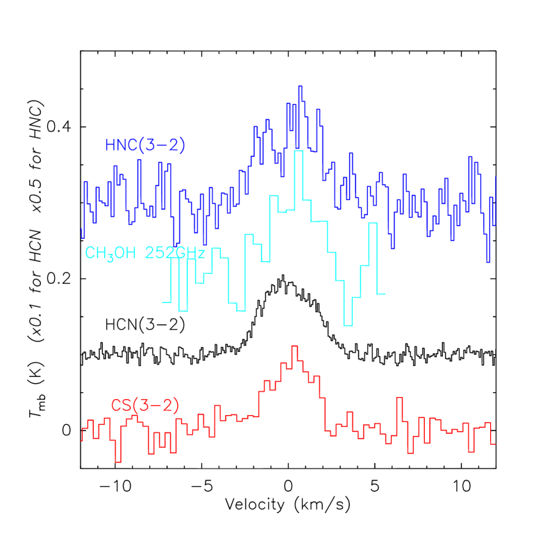
Figure 6: CS, HCN, CH${}_{3}$OH (sum of the 8 brightest lines at 252 GHz), and HNC lines observed with the IRAM 30-m telescope in comet C/2002 V1 (NEAT) on 16.5–17.6 February 2003. The spectra are plotted with the same horizontal scale to compare the line widths. The intensities of the spectra of HCN and HNC were divided by 10 and 2, respectively. Spectra are shifted vertically for clearer viewing.

2.3 C/2006 P1 (McNaught)

C/2006 P1 was discovered by Robert McNaught at $m_{v}$ = 17.3 on 7 August 2006 (iauc8737) as it was at 3.1 AU from the Sun. The geometry was very unfavorable for observing this comet as it approached the Sun. The comet was basically lost in the glare of the Sun in November and December 2006 from $r_{h}$ = 1.5 to 0.5 AU. At $r_{h}$ $>$ 0.5 AU, its intrinsic brightness was similar to that of comet C/1996 B2 (Hyakutake). It brightened rapidly in early January 2007 to peak at $m_{v}$ $\sim$ –5 and became visible to the naked eye in broad daylight (iauc8796). It passed perihelion on 12 January 2007 at $q$ = 0.17 AU. Comet C/2006 P1 (McNaught) was the brightest and most productive comet since C/1965 S1 (Ikeya-Seki). The absence of an ion tail led Ful07 to argue that, because of a very high outgassing rate, the diamagnetic cavity was so large that ions were photodissociated before reaching the region where they could interact with the solar wind. A week after perihelion, C/2006 P1 displayed a fantastic dust tail with many striae curving around 1/3 of sky at a mean distance of 20° from the Sun.

The IRAM observations were performed on 15, 16, and 17 January 2007 ($r_{h}$ = 0.21–0.25 AU). The comet ephemeris was expected to be possibly wrong by up to 1′ (corresponding to the 3-$\sigma$ uncertainty from the JPL’s HORIZONS ephemeris (horizons)). An on-the-fly map of the HCN $J$(3–2) line on 15.6 January UT with the IRAM 30-m HERA array of receivers showed that the comet was 30″ north of its predicted position (Fig. 7). Orbit updates later confirmed the observed offset (Table 1). Most observations consisted of five-point integrations at 0 and 6″  offsets in RA and Dec to pinpoint the maximum emission (e.g., Fig. 9). On 17.5 January, the observations were affected by strong anomalous refraction due to the low elevation of the comet (21–17${}^{\circ}$). The effect was estimated to be equivalent to a mean pointing offset of up to 12″, implying a loss of 90% of the signal. Observational data are summarized in Table 4.

OH 18-cm observations were performed daily between 10 and 20 January. The comet was detected intermittently. OH 18-cm lines had never been detected that close to the Sun (0.17 AU) in a comet before.

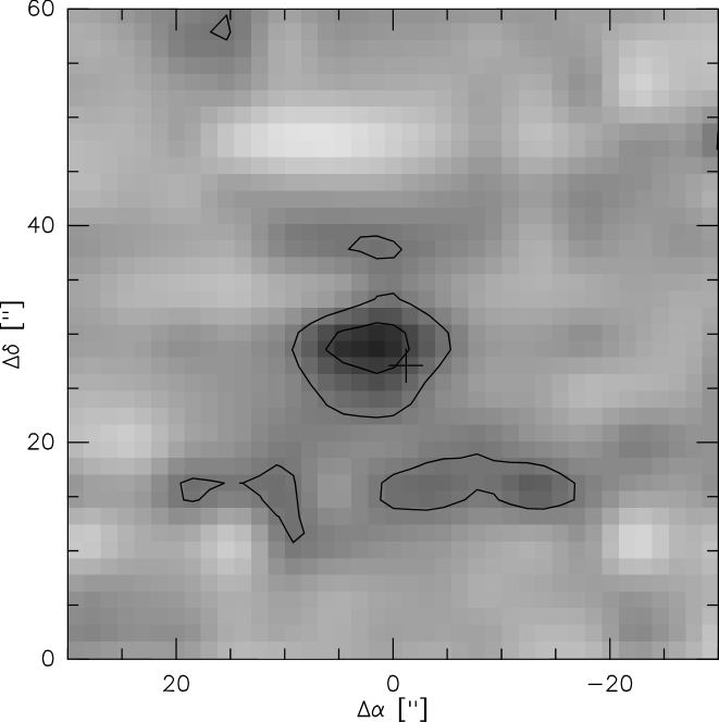
Figure 7: On-the-fly map of the HCN $J$ = 3–2 emission in comet C/2006 P1 (McNaught) obtained with the IRAM 30-m on 15.65 January 2007 (4 min. integration time). The de-pixelized image shows the line area between $-3$ and +3 km s${}^{-1}$, contour levels are 2 and 4$\sigma_{\rm rms}$. The cross marks the comet position as computed from the reference ephemeris. Before gridding to beam/2 sampling, a linear spatial baseline was subtracted from each on-the-fly subscan to remove total power fluctuations of mainly atmospheric orgin.

Figure 8: HDO line at 225.896 GHz observed with the IRAM 30-m telescope in comet C/2006 P1 on 16.6 January 2007. The vertical scale is the main-beam brightness temperature. The horizontal scale is the Doppler velocity in the comet rest-frame.

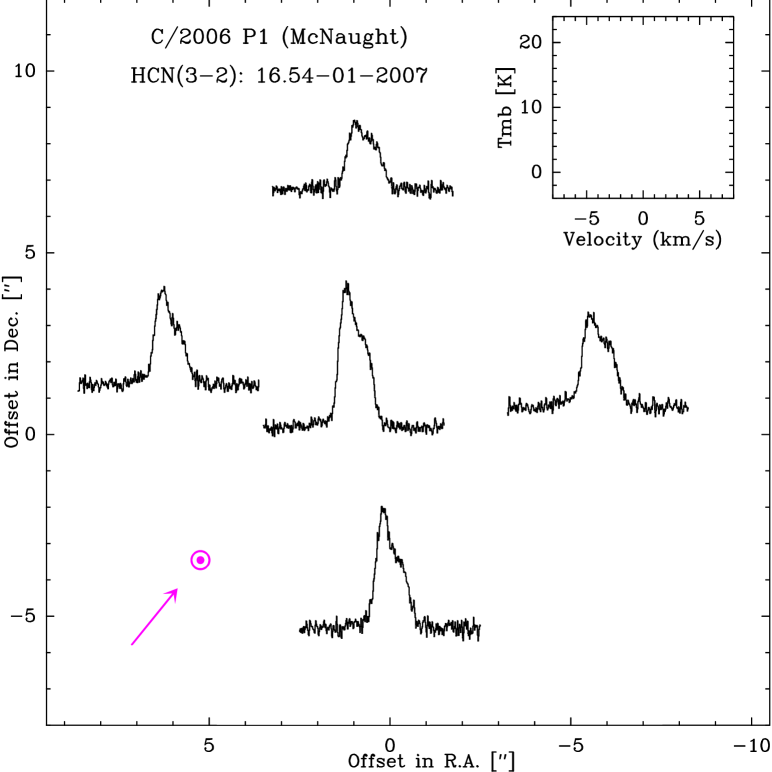
Figure 9: Coarse map of the HCN $J$(3–2) emission from comet C/2006 P1 (McNaught) on 16.5 January 2007, displayed as in Figs 1 and 5, with positions relative to the final ephemerides (Table 1).

Figure 10: CS, HCN, CH${}_{3}$OH (sum of the 4 brightest lines at 157 GHz), and HNC lines observed with the IRAM 30-m telescope in comet C/2006 P1 (McNaught) on 16.5 or 17.6 January 2007. Spectra have been plotted at the same horizontal scale to compare the line widths. The intensity scale is reduced by 10 and 2 for HCN and HNC, respectively, and shifted vertically for better viewing.

3 Analysis of Nançay data - H${}_{2}$O production rates

The characteristics of the Nançay radio telescope and the OH observations of comets may be found in Cro02. The OH 18-cm lines usually observed in comets are maser lines pumped by UV solar radiation (Des81). However, for high water-production rates, the maser emission is quenched by collisions in a large part of the coma, and most of the signal may originate from thermal emission. The radius of the region where the maser emission is quenched is estimated to be $50000r_{h}\sqrt{\rm Q_{29}}$ km, where $Q_{29}$ is the water production rate in units of $10^{29}$ molec. s${}^{-1}$ (Ger98). For production rates above $6\times 10^{29}$ molec. s${}^{-1}$ and the heliocentric distances where the comets were observed ($r_{h}<0.3$ AU), most OH radicals dissociate within the quenching zone. Hence, the signal is dominated by OH thermal emission. The OH production rates or upper limits are given in Table 5 and sample spectra are provided in Fig. 11.

Table 5 also includes water-production rate measurements from other instruments for comet C/2002 X5. The H${}_{2}$O line at 557 GHz was observed in this comet with Odin during March 2003 (Biv07a). Observations were conducted with the SOHO coronagraph spectrometer on the perihelion date: from H Lyman $\alpha$ measurements, the peak outgassing rate of water is estimated to $\sim 3\times 10^{30}$ molec. s${}^{-1}$ (Com08). According to Pov03 and Bou03, this comet displayed a strongly variable activity around perihelion with a $\sim$two day period. During the perihelion period, the comet was not or only very marginally detected at Nançay. Averaging the data obtained during the five days around perihelion, we obtain a possible 4-$\sigma$ detection (subject to baseline uncertainties) suggesting a production rate of $\sim 6\times 10^{30}$ molec. s${}^{-1}$ (Table 5). This is higher than the SOHO estimate, but still within the same order of magnitude. Power laws fitted to Nançay and Odin data (Fig. LABEL:figqp02x5) yield values in the same range 1.5–5.4$\times 10^{30}$ molec. s${}^{-1}$ at 0.214 AU from the Sun. A mean value of 3.5$\times 10^{30}$ molec. s${}^{-1}$ is adopted.

For C/2002 V1 (NEAT), the pre-perihelion observations can be fitted by a power law ($0.33\pm 0.03\times 10^{29}\times r_{h}^{-1.95\pm 0.23}$), which extrapolates to $Q_{\rm H_{2}O}=1.6\times 10^{30}$ and $2.5\times 10^{30}$ molec. s${}^{-1}$ for 16 and 17 January 2003, respectively, consistent with the upper limit determined for these days. Extrapolation of SOHO-SWAN measurements yield values that are four times higher but indicative of abundances relative to water that are abnormaly low for all molecules. We assume that $Q_{\rm H_{2}O}$ = $2.0$ and $2.5\times 10^{30}$ molec. s${}^{-1}$ , respectively, these values being more compatible with the day-to-day variations observed in millimeter spectra of other molecules.

As for C/2006 P1 (McNaught), the water production rates for 13 and 19 January deduced from the Nançay data agree with the estimated HDO production rate from the marginally detected line at 225.9 GHz (Fig. 8) and the HDO/H${}_{2}$O$=6\times 10^{-4}$ ratio measured in comets. The total production rate varied from $\approx 40\times 10^{30}$ down to $\approx 5\times 10^{30}$ molec. s${}^{-1}$ at that time (Sect.3).

2

Table 2: Molecular observations in comet C/2002 X5 (Kudo-Fujikawa)

UT date (2003)	$<r_{h}>$	$<\Delta>$	Int. time	Line	$\int T_{b}dv$	Velocity offset	offset
[mm/dd.dd–dd.dd]	[AU]	[AU]	[min]		[K km s${}^{-1}$]	[km s${}^{-1}$]
IRAM 30-m:
01/13.55–13.66	0.553	1.032	60	HCN(1-0)	$0.119\pm 0.024$	$-0.15\pm 0.25$	3.5″
01/13.55–13.66	0.553	1.032	40	HCN(3-2)	$1.405\pm 0.058$	$+0.02\pm 0.08$	3.5″
01/26.46–26.46	0.214	1.172	10	HCN(3-2)	$1.075\pm 0.190$	$+0.22\pm 0.22$	10″
01/26.47–26.49	0.214	1.172	10	HCN(3-2)	$4.640\pm 0.190$	$+0.24\pm 0.05$	6″
01/26.50–26.50	0.214	1.172	5	HCN(3-2)	$6.046\pm 0.266$	$+0.29\pm 0.09$	4.5″
01/26.51–26.57	0.213	1.172	90	HCN(3-2)	$14.268\pm 0.084$	$+0.24\pm 0.01$	1.0″
01/26.58–26.58	0.213	1.172	5	HCN(3-2)	$11.940\pm 0.335$	$+0.30\pm 0.04$	4.0″
03/12.65–12.79	1.184	1.096	90	HCN(3-2)	$0.275\pm 0.027$	$-0.16\pm 0.04$	3.0″
01/13.55–13.66	0.553	1.032	20	HNC(3-2)	$0.326\pm 0.101$	$+0.36\pm 0.40$	3.5″
01/26.46–26.46	0.214	1.172	10	HNC(3-2)	$<0.501$		13″
01/26.47–26.49	0.214	1.172	10	HNC(3-2)	$0.660\pm 0.140$	$+0.40\pm 0.26$	6.8″
01/26.50–26.57	0.213	1.172	90	HNC(3-2)	$2.415\pm 0.093$	$+0.33\pm 0.15$	2.8″
01/26.58–26.58	0.213	1.172	5	HNC(3-2)	$1.494\pm 0.399$	$+0.02\pm 0.39$	4.4″
03/12.65–12.79	1.184	1.096	90	HNC(3-2)	$<0.106$		3.0″
01/26.47–26.63	0.213	1.172	135	CH${}_{3}$CN(8,0-7,0)	$0.068\pm 0.016$	$+0.29\pm 0.25$	1.6″
				CH${}_{3}$CN(8,1-7,1)	$0.041\pm 0.015$	$-0.08\pm 0.33$
				CH${}_{3}$CN(8,2-7,2)	$0.028\pm 0.019$
				CH${}_{3}$CN(8,3-7,3)	$0.091\pm 0.019$	$-0.03\pm 0.27$
03/12.65–12.79	1.184	1.096	90	CH${}_{3}$CN(8-7)${}^{1}$	$<0.054$		3.0″
01/26.60–26.63	0.212	1.172	25	HC${}_{3}$N(28-27)	$0.700\pm 0.112$	$-0.03\pm 0.16$	1.5″
01/13.55–13.66	0.553	1.032	60	CO(2-1)	$<0.094^{1}$		3.5″
01/26.46–26.46	0.214	1.172	10	CS(3-2)	$0.278\pm 0.052$	$+0.45\pm 0.24$	10″
01/26.47–26.49	0.214	1.172	10	CS(3-2)	$0.407\pm 0.057$	$+0.23\pm 0.18$	5.5″
01/26.51–26.51	0.214	1.172	5	CS(3-2)	$0.463\pm 0.048$	$+0.04\pm 0.13$	1.5″
01/26.52–26.57	0.213	1.172	85	CS(3-2)	$0.744\pm 0.030$	$+0.31\pm 0.05$	1.3″
01/26.50–26.58	0.213	1.172	10	CS(3-2)	$0.787\pm 0.058$	$+0.10\pm 0.09$	3.7″
01/26.60–26.63	0.212	1.172	25	CS(3-2)	$0.875\pm 0.034$	$+0.25\pm 0.05$	1.5″
03/12.65–12.79	1.184	1.096	135	CS(3-2)	$<0.032$		3.0″
01/26.60–26.63	0.212	1.172	25	SiO(6-5)	$<0.516$		1.5″
01/13.55–13.66	0.553	1.032	60	CH${}_{3}$OH(1,0-1,-1)E	$0.026\pm 0.013$	$-0.51\pm 0.36$	3.5″
				CH${}_{3}$OH(2,0-2,-1)E	$0.065\pm 0.018$	$+0.58\pm 0.39$
				CH${}_{3}$OH(3,0-3,-1)E	$0.099\pm 0.018$	$-0.33\pm 0.21$
				CH${}_{3}$OH(4,0-4,-1)E	$0.049\pm 0.018$	$-0.25\pm 0.54$
				CH${}_{3}$OH(5,0-5,-1)E	$0.065\pm 0.018$	$+0.03\pm 0.34$
				CH${}_{3}$OH(6,0-6,-1)E	$0.047\pm 0.018$	$+0.25\pm 0.38$
				CH${}_{3}$OH(7,0-7,-1)E	$0.031\pm 0.018$	$+0.46\pm 0.64$
01/26.47–26.63	0.213	1.172	135	CH${}_{3}$OH(1,0-1,-1)E	$0.072\pm 0.027$	$-0.16\pm 0.38$	3.0″
				CH${}_{3}$OH(2,0-2,-1)E	$0.101\pm 0.030$	$+0.75\pm 0.41$
				CH${}_{3}$OH(3,0-3,-1)E	$0.142\pm 0.028$	$-0.28\pm 0.22$
				CH${}_{3}$OH(4,0-4,-1)E	$0.113\pm 0.030$	$-0.11\pm 0.31$
				CH${}_{3}$OH(5,0-5,-1)E	$0.197\pm 0.028$	$+0.30\pm 0.17$
				CH${}_{3}$OH(6,0-6,-1)E	$0.197\pm 0.029$	$+0.13\pm 0.17$
				CH${}_{3}$OH(7,0-7,-1)E	$0.214\pm 0.028$	$-0.10\pm 0.15$
03/12.65–12.79	1.184	1.096	135	CH${}_{3}$OH(1,0-1,-1)E	$0.042\pm 0.012$	$+0.24\pm 0.12$	3.0″
				CH${}_{3}$OH(2,0-2,-1)E	$0.024\pm 0.014$
				CH${}_{3}$OH(3,0-3,-1)E	$0.011\pm 0.013$
				CH${}_{3}$OH(4,0-4,-1)E	$0.015\pm 0.014$
				CH${}_{3}$OH(5,0-5,-1)E	$0.043\pm 0.016$	$-0.12\pm 0.15$
				CH${}_{3}$OH(6,0-6,-1)E	$0.036\pm 0.012$	$-0.03\pm 0.12$
				CH${}_{3}$OH(7,0-7,-1)E	$0.027\pm 0.012$	$-0.03\pm 0.16$
				sum of 7 lines	$0.150\pm 0.037$	$-0.01\pm 0.09$

${}^{1}$ Sum of CH${}_{3}$CN(8,0-7,0), CH${}_{3}$CN(8,1-7,1) and CH${}_{3}$CN(8,2-7,2) lines.

3

Table 3: Molecular observations in comet C/2002 V1 (NEAT)

UT date (2003)	$<r_{h}>$	$<\Delta>$	Int. time	Line	$\int T_{b}dv$	Velocity offset	offset
[mm/dd.dd–dd.dd]	[AU]	[AU]	[min]		[K km s${}^{-1}$]	[km s${}^{-1}$]
IRAM 30-m:
02/16.49–16.59	0.136	0.978	50	HCN(3-2)	$4.146\pm 0.061$	$-0.02\pm 0.03$	1.8″
	0.136	0.978	19	HCN(3-2)	$2.173\pm 0.112$	$-0.01\pm 0.11$	5.1″
02/17.48–17.52	0.108	0.985	19	HCN(3-2)	$3.558\pm 0.069$	$+0.01\pm 0.04$	1.8″
02/17.48–17.50	0.109	0.985	9	HCN(3-2)	$1.819\pm 0.140$	$-0.18\pm 0.17$	5.7″
02/17.55–17.66	0.106	0.987	85	HCN(1-0)	$0.116\pm 0.021$	$+0.06\pm 0.32$	1.8″
02/16.49–16.59	0.135	0.978	29	HNC(3-2)	$0.648\pm 0.113$	$+0.09\pm 0.35$	5.5″
02/16.49–16.66	0.134	0.978	85	HNC(3-2)	$0.914\pm 0.060$	$+0.25\pm 0.13$	2.8″
02/16.49–16.59	0.135	0.978	27	CS(3-2)	$0.242\pm 0.054$	$+0.57\pm 0.42$	5.5″
02/16.49–16.66	0.134	0.978	87	CS(3-2)	$0.336\pm 0.026$	$+0.05\pm 0.13$	2.8″
02/17.48–17.52	0.108	0.985	22	CS(3-2)	$0.373\pm 0.046$	$-0.34\pm 0.21$	1.7″
02/17.48–17.50	0.109	0.985	6	CS(3-2)	$0.180\pm 0.085$		5.6″
02/16.49–17.50	0.130	0.980	22	CH${}_{3}$CN(8-7)${}^{1}$	$<0.126$		2.5″
02/17.61–17.66	0.106	0.987	35	CO(2-1)	$<0.161$		2.8″
02/16.54–17.66	0.120	0.982	80	OCS(12-11)	$<0.029$		2.1″
				HC${}_{3}$N(16-15)	$<0.031$		2.1″
				H${}_{2}$CO($2_{02}-1_{01}$)	$0.032\pm 0.012$		2.1″
02/17.55–17.60	0.107	0.986	50	H${}_{2}$CO($3_{12}-2_{11}$)	$<0.136$		1.0″
02/16.60–17.60	0.120	0.982	107	CH${}_{3}$OH(3,3-3,2)A${}^{\pm\leavevmode\nobreak\ 2}$	$0.072\pm 0.045$		1.8″
				CH${}_{3}$OH(4,3-4,2)A${}^{\pm}$	$0.213\pm 0.046$	$+0.20\pm 0.35$
				CH${}_{3}$OH(5,3-5,2)A${}^{\pm}$	$0.092\pm 0.044$
				CH${}_{3}$OH(6,3-6,2)A${}^{\pm}$	$0.182\pm 0.047$	$+0.31\pm 0.48$
				CH${}_{3}$OH(7,3-7,2)A${}^{\pm}$	$0.198\pm 0.041$	$-0.28\pm 0.29$
				CH${}_{3}$OH(8,3-8,2)A${}^{\pm}$	$0.057\pm 0.041$
02/16.60–17.60	0.120	0.982	107	SO($5_{6}-4_{5}$)	$<0.071$		1.8″
02/17.61–17.66	0.106	0.987	35	SiO(6-5)	$<0.190$		1.7″

${}^{1}$: sum of CH${}_{3}$CN(8,0-7,0), CH${}_{3}$CN(8,1-7,1), CH${}_{3}$CN(8,2-7,2) and CH${}_{3}$CN(8,3-7,3) lines.;
${}^{2}$: sums of twin lines;

4

Table 4: Molecular observations in comet C/2006 P1 (Mc Naught)

UT date (2007)	$<r_{h}>$	$<\Delta>$	Int. time	Line	$\int T_{b}dv$	Velocity offset	offset
[mm/dd.dd–dd.dd]	[AU]	[AU]	[min]		[K km s${}^{-1}$]	[km s${}^{-1}$]
IRAM 30-m:
01/15.65	0.207	0.817	0.1	HCN(3-2)	$83.74\pm 7.63$	$-0.27\pm 0.16$	2.6″
	0.207	0.817	0.2	HCN(3-2)	$57.66\pm 5.82$	$+0.33\pm 0.18$	5.0″
	0.207	0.817	2.0	HCN(3-2)	$31.78\pm 3.07$	$+0.40\pm 0.18$	7.4″
	0.207	0.817	0.3	HCN(3-2)	$22.89\pm 5.08$	$-0.21\pm 0.38$	8.9″
	0.207	0.817	0.8	HCN(3-2)	$13.76\pm 3.32$	$+0.33\pm 0.44$	12.1″
01/16.53	0.228	0.821	8.0	HCN(3-2)	$48.45\pm 0.42$	$-0.07\pm 0.02$	4.9″
01/16.54	0.228	0.821	8.0	HCN(3-2)	$63.65\pm 0.39$	$-0.09\pm 0.01$	2.1″
01/16.55	0.228	0.821	20.0	HCN(3-2)	$37.47\pm 0.26$	$-0.06\pm 0.02$	6.5″
01/16.54	0.228	0.821	4.0	HCN(3-2)	$27.28\pm 0.57$	$-0.03\pm 0.05$	8.2″
01/16.58	0.229	0.822	12.0	HCN(3-2)	$47.89\pm 0.28$	$-0.03\pm 0.01$	4.7″
01/16.59	0.229	0.822	8.0	HCN(3-2)	$16.60\pm 0.33$	$+0.04\pm 0.05$	9.3″
01/17.55	0.255	0.832	2.0	HCN(3-2)	$35.91\pm 0.59$	$-0.05\pm 0.04$	3.3″
01/17.54	0.255	0.832	10.0	HCN(3-2)	$21.81\pm 0.28$	$-0.02\pm 0.03$	5.3″
01/17.56	0.255	0.833	31.0	HCN(3-2)	$15.58\pm 0.16$	$+0.04\pm 0.02$	7.1″
01/17.55	0.255	0.832	5.0	HCN(3-2)	$14.44\pm 0.40$	$-0.02\pm 0.06$	8.5″
01/17.58	0.256	0.833	20.0	HCN(3-2)	$6.72\pm 0.22$	$-0.04\pm 0.07$	10.7″
01/17.58	0.256	0.833	12.0	HCN(3-2)	$5.69\pm 0.27$	$-0.06\pm 0.11$	12.4″
01/16.54	0.228	0.821	20.0	HCN(1-0)	$1.723\pm 0.057$	$+0.16\pm 0.05$	3.9″
01/16.55	0.228	0.821	16.0	HCN(1-0)	$1.505\pm 0.066$	$+0.02\pm 0.06$	6.8″
01/16.54	0.228	0.821	4.0	HCN(1-0)	$1.574\pm 0.131$	$-0.13\pm 0.11$	8.1″
01/16.59	0.229	0.822	12.0	HCN(1-0)	$1.920\pm 0.031$	$-0.01\pm 0.02$	4.8″
01/16.59	0.229	0.822	8.0	HCN(1-0)	$1.261\pm 0.037$	$-0.08\pm 0.03$	10.2″
01/17.55	0.255	0.832	2.0	HNC(3-2)	$4.05\pm 0.55$	$-0.06\pm 0.18$	3.7″
01/17.54	0.255	0.832	9.0	HNC(3-2)	$3.16\pm 0.24$	$+0.03\pm 0.09$	4.7″
01/17.56	0.255	0.833	23.0	HNC(3-2)	$1.53\pm 0.16$	$+0.11\pm 0.12$	6.7″
01/17.54	0.255	0.832	14.0	HNC(3-2)	$1.52\pm 0.20$	$+0.13\pm 0.16$	9.1″
01/17.54	0.255	0.832	8.0	HNC(3-2)	$0.52\pm 0.26$		11.5″
01/17.55	0.255	0.832	2.0	CS(3-2)	$2.84\pm 0.20$	$+0.07\pm 0.08$	3.4″
01/17.54	0.255	0.832	8.0	CS(3-2)	$2.47\pm 0.10$	$-0.04\pm 0.04$	4.7″
01/17.56	0.255	0.833	24.0	CS(3-2)	$1.53\pm 0.06$	$-0.03\pm 0.04$	6.8″
01/17.54	0.255	0.832	13.0	CS(3-2)	$1.17\pm 0.08$	$-0.09\pm 0.08$	9.1″
01/17.54	0.255	0.832	9.0	CS(3-2)	$1.01\pm 0.09$	$+0.11\pm 0.10$	11.4″
01/17.51–17.58	0.255	0.832	47	CH${}_{3}$CN(8,0-7,0)	$0.148\pm 0.040$	$+0.45\pm 0.20$	6.9″
				CH${}_{3}$CN(8,1-7,1)	$0.080\pm 0.044$	$-0.60\pm 0.47$
				CH${}_{3}$CN(8,2-7,2)	$0.004\pm 0.039$
				CH${}_{3}$CN(8,3-7,3)	$0.104\pm 0.042$	$-1.01\pm 0.62$
				Sum of the 4 lines	$0.334\pm 0.083$
01/16.52–16.60	0.228	0.821	48	CH${}_{3}$OH(1,0-1,-1)E	$0.203\pm 0.050$		4.9″
				CH${}_{3}$OH(2,0-2,-1)E	$0.160\pm 0.047$	$-0.52\pm 0.44$
				CH${}_{3}$OH(3,0-3,-1)E	$0.309\pm 0.050$
				CH${}_{3}$OH(4,0-4,-1)E	$0.327\pm 0.048$	$-0.06\pm 0.21$
				CH${}_{3}$OH(5,0-5,-1)E	$0.305\pm 0.047$	$+0.14\pm 0.22$
				CH${}_{3}$OH(6,0-6,-1)E	$0.347\pm 0.047$	$-0.05\pm 0.20$
				CH${}_{3}$OH(7,0-7,-1)E	$0.297\pm 0.042$	$-0.24\pm 0.20$
01/16.54–16.60	0.228	0.821	8	CH${}_{3}$OH($J,0-J,-1$)E${}^{1}$	$0.857\pm 0.198$	$-0.60\pm 0.35$	8.9″
01/17.51–17.58	0.255	0.832	48	CH${}_{3}$OH(1,0-1,-1)E	$0.024\pm 0.035$		6.7″
				CH${}_{3}$OH(2,0-2,-1)E	$-0.021\pm 0.039$
				CH${}_{3}$OH(3,0-3,-1)E	$0.081\pm 0.035$
				CH${}_{3}$OH(4,0-4,-1)E	$0.028\pm 0.042$	$+0.64\pm 0.60$
				CH${}_{3}$OH(5,0-5,-1)E	$0.095\pm 0.040$	$-0.47\pm 0.46$
				CH${}_{3}$OH(6,0-6,-1)E	$0.103\pm 0.045$	$-0.17\pm 0.47$
				CH${}_{3}$OH(7,0-7,-1)E	$0.082\pm 0.040$	$-0.55\pm 0.40$
				CH${}_{3}$OH($J,0-J,-1$)E${}^{1}$	$0.380\pm 0.079$	$-0.40\pm 0.29$	6.7″
01/16.52–16.60	0.228	0.821	60	H${}_{2}$CO($3_{12}-2_{11}$)	$0.334\pm 0.050$	$-0.18\pm 0.20$	6.1″
01/16.52–16.59	0.228	0.821	36	HDO($3_{12}-2_{11}$)	$0.227\pm 0.064$	$-0.68\pm 0.40$	4.2″
01/15.60	0.207	0.817	5.0	CO(2-1)	$<2.31$		12.1″
01/17.59–17.61	0.256	0.833	24	CO(2-1)	$0.30\pm 0.09$	$-0.07\pm 0.43$	11.2″
01/17.59–17.61	0.256	0.833	24	HCO+(1-0)	$0.36\pm 0.05$	$-0.05\pm 0.27$	10.9″

${}^{1}$: sum of CH${}_{3}$OH lines $J,K$ = (4,0-4,-1)E, (5,0-5,-1)E, (6,0-6,-1)E and (7,0-7,-1)E.

The estimated visual magnitudes of these comets at perihelion were $m_{1}\approx+3$, $m_{1}\approx-1.5$, and $m_{1}\approx-5$ for C/2002 X5, C/2002 V1, and C/2006 P1, respectively. Correcting for the $-2$ magnitude surge in brightness of C/2006 P1 caused by forward scattering (Mar07), and using the correlation law between heliocentric magnitude and $Q_{\rm H_{2}O}$ of Jor08, this would imply water production rates of 1, 11, and 26$\times 10^{30}$ molec. s${}^{-1}$ respectively. The comparison to measured production rates in Table 5 suggests that C/2002 V1 was a more dusty comet than the two others since, unlike C/2002 X5 and C/2006 P1, the actual outgassing rate being much lower than the value ($11\times 10^{30}$ molec. s${}^{-1}$ ) inferred from visual magnitudes.

Figure 11: Nançay spectra of OH 18-cm lines (average of 1665 and 1667 MHz transitions) corresponding to observations listed in Table 5.

Table 5: Water production rates

UT date	$<r_{h}>$	Observatory	Line intensity	$Q_{\rm H_{2}O}$	Ref.
[mm/dd.dd]	[AU]	and line	[mJy km s${}^{-1}$]	[molec. s${}^{-1}$ ]
C/2002 X5 (Kudo-Fujikawa): (2003)
01/12.5–14.5	0.55	Nançay OH 18-cm	$-156\pm 7$	$1.5\pm 0.1\times 10^{29}$
01/15.5–19.5	0.45	Nançay OH 18-cm	$-91\pm 5$	$1.8\pm 0.1\times 10^{29}$
01/26.50	0.214	Nançay OH 18-cm	$47\pm 15$	$85\pm 27\times 10^{29}$
01/25.5–30.5	0.205	Nançay OH 18-cm	$\approx 32\pm 8$	$\approx 64\pm 16\times 10^{29}$
01–02	$<1$	SOHO-SWAN	-	$0.56\times 10^{29}\times r_{h}^{-2.0}$	[3]
01/27.92	0.195	SOHO-UVCS Lyman $\alpha$	-	$5.5\times 10^{29}$	[1]
01/28.13	0.194	SOHO-UVCS Lyman $\alpha$	-	$9.0\times 10^{29}$	[1]
01/28.79	0.190	SOHO-UVCS Lyman $\alpha$	-	$13.0\times 10^{29}$	[1]
01/29.17	0.190	SOHO-UVCS Lyman $\alpha$	-	$27.0\times 10^{29}$	[1]
03/12.5	1.178	Odin H${}_{2}$O 557GHz	$879\pm 79^{1}$	$0.21\pm 0.01\times 10^{29}$	[2]
C/2002 V1 (NEAT): (2003)
01/00–07	1.30	Nançay OH 18-cm	$-25\pm 4$	$0.15\pm 0.02\times 10^{29}$
01/08–14	1.15	Nançay OH 18-cm	$-45\pm 4$	$0.24\pm 0.02\times 10^{29}$
01/15–19	1.01	Nançay OH 18-cm	$-81\pm 5$	$0.46\pm 0.03\times 10^{29}$
01/21–25	0.87	Nançay OH 18-cm	$-110\pm 6$	$0.55\pm 0.03\times 10^{29}$
01/26–30	0.73	Nançay OH 18-cm	$-93\pm 5$	$0.59\pm 0.03\times 10^{29}$
02/01–05	0.59	Nançay OH 18-cm	$-85\pm 6$	$0.70\pm 0.06\times 10^{29}$
02/06–09	0.45	Nançay OH 18-cm	$-66\pm 7$	$1.7\pm 0.2\times 10^{29}$
02/16.50	0.136	Nançay OH 18-cm	$-2\pm 13$	$<150\times 10^{29}$
01–03	$<1$	SOHO-SWAN	-	$0.94\times 10^{29}\times r_{h}^{-2.1}$	[3]
C/2006 P1 (McNaught): (2007)
01/12.51	0.171	Nançay OH 18-cm	$45\pm 23$	$<270\times 10^{29}$
01/13.51	0.173	Nançay OH 18-cm	$111\pm 15$	$400\pm 60\times 10^{29}$
01/17.52	0.254	Nançay OH 18-cm	$-9\pm 23$	$<100\times 10^{29}$
01/19.52	0.311	Nançay OH 18-cm	$128\pm 26$	$80\pm 20\times 10^{29}$

${}^{1}$: line integrated intensity in mK km s${}^{-1}$;
[1]: Pov03; [2]: Biv07a; [3]: Com08

4 Analysis of IRAM data

Molecular production rates were derived using models of molecular excitation and radiation transfer (Biv99; Biv00; Biv06a). The excitation model of CH${}_{3}$OH was updated. The computation of the partition function considers now the first torsional state, which is populated significantly in the hot atmospheres of the comets studied in this paper. For these productive comets observed at small $r_{h}$, a significant fraction of the observed molecules are photodissociated before leaving the collision-dominated region. Thus, the determination of the gas kinetic temperature (which controls the rotational level populations in the collision zone) and strong constraints on molecular lifetimes were essential. As shown below, line shapes and brightness distributions obtained from coarse maps provide information on the gas outflow velocity and molecular lifetimes.

4.1 Gas temperature

Table 6 summarizes rotational temperatures deduced from relative line intensities. Using our excitation models, we then constrained the gas temperature (Table 6) following the methods outlined in, e.g., Biv99. Several data are indicative of relatively high temperatures, which are difficult to measure because the rotational population is spread over many levels making individual lines weaker. Hence, the uncertainties in derived values are high. We note that the values derived for C/2002 X5 from CH${}_{3}$OH lines do not reflect the marginal detection of some lines. The inconsistency between the different measurements, especially from CH${}_{3}$OH and HCN lines in comet C/2006 P1, is possibly related to differences in collision cross-sections and temperature variations in the coma.

Gas temperature laws as a function $r_{h}$ were obtained for comets C/1995 O1 (Hale-Bopp) (Biv02b), C/1996 B2 (Hyakutake) (Biv99), and 153P/Ikeya-Zhang (Biv06a). The laws ($100r_{h}^{-1.1}$ for Hale-Bopp and $60r_{h}^{-0.9}$ for other comets on average), extrapolate to $T=200$–1000 K for $r_{h}=0.25$–0.11 AU. Photolytic heating increases with decreasing $r_{h}$ and the increasing production rate of water. Hence, we expect higher temperatures for the most productive comet C/2006 P1. Com88 predicted a maximum temperature on the order of 500–900 K for comet Kohoutek at 0.25–0.14 AU, but temperatures are generally below 300 K at distances from the nucleus where molecules are not photodissociated. Given also that the HCN $J$(3–2) $v_{2}=1$ line at 265852.709 MHz is not detected, we estimate that temperatures are lower than 300 K below $r_{h}$=0.25 AU.

For C/2002 X5, we adopted the gas kinetic temperature values of 50 K, 180 K, and 40 K for mid-January, end of January, and mid-March all in 2003, respectively. For C/2002 V1 and C/2006 P1, we used 150 K and 300 K, respectively. We later discuss (in Sect. 5.1) the influence of the assumed temperature on the inferred production rates.

Table 6: Gas temperature measurements

UT date	$<r_{h}>$	offset	Lines	Rotational temperature	Gas temperature
[mm/dd.dd]	[AU]	[″]		[K]	[K]
C/2002 X5 (Kudo-Fujikawa): (2003)
01/13.61	0.553	3.5	CH${}_{3}$OH 157 GHz	$38\pm 10$	$30\pm 10$
01/26.54	0.213	3.0	CH${}_{3}$OH 157 GHz	$320^{+\infty}_{-170}$	$175^{+\infty}_{-90}$
01/26.54	0.213	1.6	CH${}_{3}$CN 147 GHz	$1500^{+\infty}_{-1305}$	$>190$
01/26.54	0.213	1.0	HCN$J$(3–2),$v_{2}=1/v_{2}=0$	$<245$	$<530^{1}$
03/12.72	1.184	3.0	CH${}_{3}$OH 157 GHz	$85^{+68}_{-25}$	$70^{+50}_{-20}$
C/2002 V1 (NEAT): (2003)
02/17.0	0.120	1.9	HCN$J$(3–2),$v_{2}=1/v_{2}=0$	$<285$	$<574^{1}$
02/17.25	0.116	1.6	CH${}_{3}$OH 252 GHz	$83^{+77}_{-27}$	$80^{+80}_{-30}$
02/17.3	0.110	1.6	CH${}_{3}$OH 252 GHz+$20_{3}$A${}^{+-}$	$228^{+92}_{-51}$	$220^{+90}_{-50}$
02/17.6	0.108	1.8	HCN$J$(3–2)/(1–0)	$54^{+60}_{-22}$	$80^{+95}_{-35}$
C/2006 P1 (McNaught): (2007)
01/16.56	0.228	3	HCN$J$(3–2)/(1–0)	299${}^{+\infty}_{-204}$ ${}^{2}$	$>375$ ${}^{2}$
01/16.56	0.228	5	HCN$J$(3–2)/(1–0)	$>168$ ${}^{2}$	$>600$ ${}^{2}$
01/16.55	0.229	5.9	CH${}_{3}$OH 157 GHz	$149^{+\infty}_{-77}$	$110^{+\infty}_{-50}$
01/16.56	0.229	4.9	CH${}_{3}$OH 157 GHz	$88^{+32}_{-19}$	$70^{+20}_{-10}$
01/17.5	0.255	6.5	HCN$J$(3–2),$v_{2}=1/v_{2}=0$	$<278$	$<677^{1}$
01/17.55	0.255	6.7	CH${}_{3}$OH 157 GHz	$>130$	$>90$
01/17.55	0.255	6.9	CH${}_{3}$CN 147 GHz	$78^{+106}_{-28}$	$80^{+110}_{-30}$

${}^{1}$ A significant fraction of the molecules are outside the collisional region and a higher gas temperature is needed to populate the $v=1$ level inside the collision zone.

${}^{2}$ A 10% calibration uncertainty in each line is assumed.

4.2 Screening of photolysis by water molecules

Given high water-production rates ($>10^{30}$–10${}^{31}$ molec. s${}^{-1}$ ), self-shielding against photodissociation by solar UV radiation is significant for these comets. As a consequence, molecules can have longer lifetimes on the night side, and reduced H${}_{2}$O photolysis may limit gas acceleration. We studied the screening of photolysis using simplified assumptions: isotropic outgassing at a constant expansion velocity and an infinite lifetime for the screening molecules (i.e., we assumed that their scale length is larger than the size of the optically thick region). According to Nee85, when considering Lee86 and Lee84, the OH photoabsorption cross-section does not differ much from the H${}_{2}$O one: it peaks close to the Lyman $\alpha$ wavelength and is slightly stronger (1–2 times). On the other hand, the cometary hydrogen may not absorb significantly the Solar Lyman $\alpha$ spectral line. The comet Lyman $\alpha$ line is too narrow (velocity dispersion of 20 km s${}^{-1}$) to absorb significantly the solar emission ($\approx$180 km s${}^{-1}$  line width). Consequently, if the sum of the scalelengths of H${}_{2}$O and OH is larger than the distances from the nucleus considered hereafter, the infinite lifetime assumption should not underestimate the screening effect.

In cylindrical coordinates, with the vertical z-axis pointing towards the Sun, a point in the coma has coordinates ($\theta$, $\rho=r\sin(\phi)$, $z_{r}=r\cos(\phi)$), where $r$ is the distance to the nucleus and $\phi$ the co-latitude angle. The photodissociation rate of a molecule M, characterized by its photodissociation absorption cross-section $\sigma_{\rm M}(\lambda)$, in a radiation field $F(\lambda)$ (in photons m${}^{-2}$ s${}^{-1}$ nm${}^{-1}$) is given by

$$\beta_{M}=\int_{\lambda}\sigma_{\rm M}(\lambda)F(\lambda)d\lambda.$$ (1)

The problem is symmetric around the z-axis. At ($\rho$, $z_{r}$), the solar flux at wavelength $\lambda$ will be attenuated to

$$F(\lambda,\rho,\phi)=F_{0}(\lambda)\exp[-\tau(\lambda,\rho,\phi)]$$ (2)

because of the optical thickness along the comet-sun axis. We consider water as the major molecule responsible for the opacity, which is connected to its absorption cross-section $\sigma_{\rm H_{2}O}(\lambda)$ by

$$\tau(\lambda,\rho,\phi)=\sigma_{\rm H_{2}O}(\lambda)\int_{z_{r}}^{\infty}n_{\rm H_{2}O}(\rho,z)dz.$$ (3)

The photons absorbed are mostly those responsible for photodissociation and not fluorescence. Photodissociation of molecules takes place for $\lambda<200$ nm and a significant solar UV field ($\lambda>80$ nm). Using the assumptions for the density, we can integrate the density along the z-axis to obtain

$$\int_{z_{r}}^{\infty}n_{\rm H_{2}O}(\rho,z)dz = \int^{\infty}_{z_{r}=\rho/\tan(\phi)}\frac{Q_{\rm H_{2}O}}{4\pi v_{\rm exp}(\rho^{2}+z^{2})}dz$$

$$= \frac{Q_{\rm H_{2}O}}{4\pi v_{\rm exp}r}\frac{\phi}{\sin(\phi)}.$$

Hence at any point in the coma, we estimate the opacity

$$\tau(\lambda,r,\phi)=<\tau(\lambda,r)>\frac{4\phi}{\pi^{2}\sin(\phi)}=C(\lambda)\frac{\phi}{r\sin(\phi)},$$ (4)

where the average value of the opacity over $4\pi$ steradians at the distance $r$ from the nucleus is

$$<\tau(\lambda,r)>=C(\lambda)\frac{\pi^{2}}{4}\frac{1}{r}$$ (5)

with

$$C(\lambda)=\frac{\sigma_{\rm H_{2}O}(\lambda)Q_{\rm H_{2}O}}{4\pi v_{\rm exp}}.$$ (6)

The surface corresponding to an opacity $\tau(\lambda,r,\phi)=1.0$ is defined by

$$r_{thick}(\phi)=C(\lambda)\frac{\phi}{sin(\phi)}=\frac{\sigma_{\rm H_{2}O}(\lambda)Q_{\rm H_{2}O}}{4\pi v_{\rm exp}}\frac{\phi}{\sin(\phi)}.$$ (7)

According to Eq. 7, the size of the optically thick region tends to infinity in the anti-sunward direction ($\phi=\pi$). It has a finite length determined by the apparent size of the Sun (2.7° at $r_{h}=0.2$ AU). This region is plotted in Fig. LABEL:figgeom for the three comets, considering only absorption of Lyman $\alpha$ photons by water molecules with a cross-section $\sigma_{\rm H_{2}O}(Ly\leavevmode\nobreak\ \alpha)$ = $15\times 10^{-22}$ m${}^{2}$ (Lew83).

We next consider HCN photodissociation, but similar equations can be established for other molecules. The effective HCN photodissociation rate at a point ($r$,$\phi$) in the coma can then be derived from Eq. 1

$$\beta_{\rm HCN}(r,\phi)=\int_{\lambda}\sigma_{\rm HCN}(\lambda)F_{0}(\lambda)\exp\left(-\frac{C(\lambda)\phi}{r\sin(\phi)}\right)d\lambda,\\$$ (8)

where $\sigma_{\rm HCN}(\lambda)$ is the photodissociation cross-section for HCN. The integration can be divided over several wavelength intervals, corresponding to the different absorption bands of HCN and H${}_{2}$O

$$\beta_{\rm HCN}(r,\phi) = \sum_{\lambda_{i}}\beta_{\rm HCN,\lambda_{i}}(r,\phi)$$

$$= \beta_{0,\rm HCN}\times\sum_{\lambda_{i}}x_{i}\exp\left(-C(\lambda_{i})\frac{\phi}{r\sin(\phi)}\right),$$

where $x_{i}$ corresponds to the fraction of the photodissociation rate due to radiation around the wavelength $\lambda_{i}$. For HCN, 88% of the contribution comes from solar Lyman $\alpha$, i.e., $x_{\rm Ly\leavevmode\nobreak\ \alpha}=0.88$ (Boc85). To ease computations, we make the approximation

$$\sum_{\lambda_{i}}x_{i}\exp\left(-\frac{C(\lambda_{i})\phi}{r\sin(\phi)}\right)\approx\exp\left(-\sum_{\lambda_{i}}\frac{x_{i}C(\lambda_{i})\phi}{r\sin(\phi)}\right).$$ (9)

This rough assumption is valid for small opacities ($r>r_{thick}$) and if the water absorption cross-sections are the same at all wavelengths $\lambda_{i}$. Otherwise, it will slightly overestimate the screening effect in the opaque region. We then define an effective water absorption cross-section for HCN (likewise for the other molecules)

$$<\sigma_{\rm H_{2}O\rightarrow HCN}>=\sum_{\lambda_{i}}x_{i}\sigma_{\rm H_{2}O}(\lambda_{i})=13.8\times 10^{-22}\leavevmode\nobreak\ {\rm m}^{2},$$ (10)

where most of the contribution comes from Lyman $\alpha$ ($\sigma_{\rm H_{2}O}(Ly\leavevmode\nobreak\ \alpha)=15\times 10^{-22}$ m${}^{2}$, Lee86; Lew83). This approximation was validated by ourselves for HCN: we estimated numerically that using this mean value for the screening cross-section instead of summing over various wavelength intervals yields only a $\approx 2$% excess error in the estimate of the increase in the number of molecules due to screening.

After solving the differential balance equation for the HCN density at the distance $r$ from the nucleus in the coma, we find that

$$n_{\rm HCN}(r,\phi)=\frac{Q_{\rm HCN}}{4\pi v_{\rm exp}r^{2}}\exp\left(-\frac{r\beta_{0}}{v_{\rm exp}}G(\frac{r}{C_{\rm HCN}\frac{\phi}{\sin(\phi)}})\right)$$ (11)

with

$$C_{\rm HCN}=\frac{<\sigma_{\rm H_{2}O\rightarrow HCN}>Q_{\rm H_{2}O}}{4\pi v_{\rm exp}}.$$ (12)

The function $G(x)=\frac{1}{x}\int_{0}^{x}\exp(-1/t)dt$ is equal to the exponential integral $G(x)$= E${}_{2}(1/x)$, which can easily be computed by numerical integration. We note that $G(\infty)=1.0$, so that Eq. 11 gives the classical Haser formula for negligible opacities.

We compared the production rates determined using the density from Eq. 11 to those obtained with the Haser formula. The largest effect is for comet C/2006 P1 with a $\approx$ 60% decrease of the HCN production rate, and $\approx$ 40% decrease for CH${}_{3}$OH, CH${}_{3}$CN, or HDO. We did not develop a full 3-D model to take into account phase angles different from 0°  or 180°. But the comparison between the case of a phase angle of 180° , where we can simply use Eq. 11, and replacing Eq. 4 by the averaged value in Eq. 5, only yields a 3% difference.

Table 7 provides characteristic scalelengths for the three comets and for comparison C/1996 B2 (Hyakutake) and C/1995 O1 (Hale-Bopp) observed in 1996–1997. In all cases, the optically thick region (at the Lyman $\alpha$ wavelength) is within the water coma ($L_{\rm H_{2}O}>$ $\langle r_{thick}(Ly\leavevmode\nobreak\ \alpha)\rangle$) and if one takes into account OH, the assumption of an infinite lifetime for the screening molecules is valid since the coma encompassing H${}_{2}$O and OH is definitely larger than the optically thick region and the HCN coma. One can also note that for comets C/1996 B2 and C/1995 O1, $L_{\rm HCN}\gg$ $\langle r_{thick}(Ly\leavevmode\nobreak\ \alpha)\rangle$, so that the screening effect is negligible.

Table 7: Typical scale lengths affected by screening

Comet	$<r_{h}>$	$Q_{\rm H_{2}O}$	$v_{\rm exp}$	$L_{\rm H_{2}O}$	$L_{\rm OH}$	$<r_{thick}(\rm Ly\leavevmode\nobreak\ \alpha)>$	$L_{\rm HCN}$
	[AU]	[$10^{29}s^{-1}$]	[km s${}^{-1}$]	[km]	[km]	[km]	[km]
C/1996 B2 (Hyakutake)	0.25	5	1.60	7900	14300	90	6600
C/1995 O1 (Hale-Bopp)	0.91	100	1.10	70000	128000	2700	58000
C/2002 X5 (Kudo-Fujikawa)	0.21	35	1.25	3600	7200	820	2900
C/2002 V1 (NEAT)	0.12	20	2.00	2000	3800	300	1600
C/2006 P1 (McNaught)	0.23	300	1.50	8100	14900	5900	4900

$L_{\rm H_{2}O}$, $L_{\rm OH}$, $L_{\rm HCN}$: unscreened scale lengths of H${}_{2}$O, OH, and HCN, taking into account solar activity, expansion velocity, and heliocentric distance.
$<r_{thick}(\rm Ly\leavevmode\nobreak\ \alpha)>$: mean radius of the optically thick Lyman $\alpha$ envelope ($\frac{\pi^{2}}{4}C(\rm Ly\leavevmode\nobreak\ \alpha)$).